The normalization model predicts responses in the human visual cortex during object-based attention
- School of Cognitive Sciences, Institute for Research in Fundamental Sciences, Iran
- School of Electrical Engineering, University of Tehran, Iran
- Laboratory of Brain and Cognition, National Institute of Mental Health, United States
Figures
Figure 1 with 1 supplement
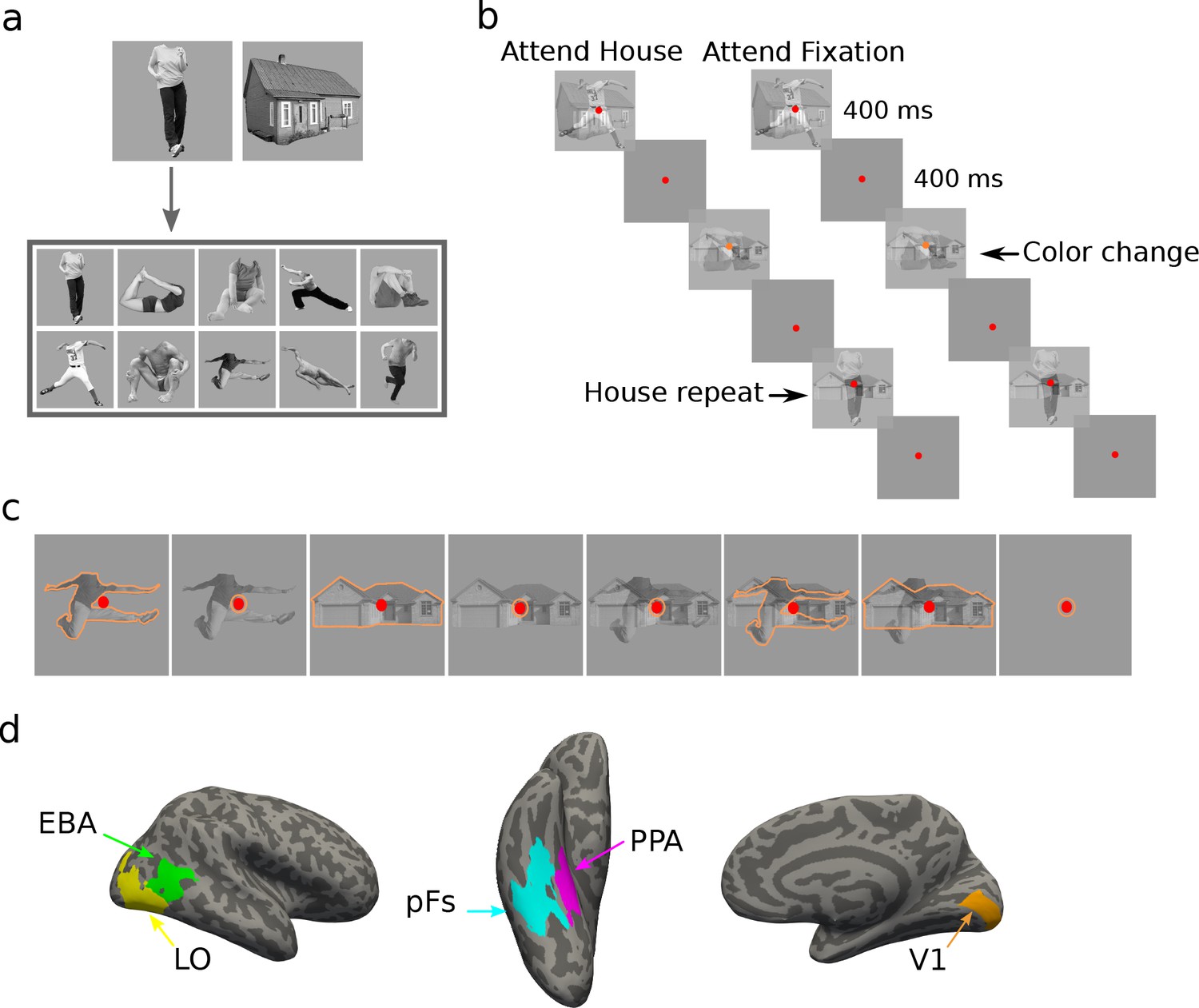
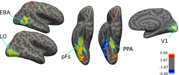
Stimuli, paradigm, and regions of interest.
(a) The two stimulus categories (body and house), with the ten exemplars of the body category. (b) Experimental paradigm including the timing of the trials and the inter-stimulus interval. In the example block depicted on the left, both stimulus categories were presented, and the participant was cued to attend to the house category. The two stimuli were superimposed in each trial, and the participant had to respond when the same stimulus from the house category appeared in two successive trials. The color of the fixation point randomly changed in some trials from red to orange, but the participants were asked to ignore the color change. The example block depicted on the right illustrates the condition in which stimuli were ignored and participants were asked to attend to the fixation point color, and respond when they detected a color change. Subjects were highly accurate in performing these tasks (see Figure 1—figure supplement 1). (c) The eight task conditions in each experimental run. For illustration purposes, we have shown the attended category in each block with orange outlines. The outlines were not present in the actual experiment. (d) Regions of interest for an example participant, including the primary visual cortex V1, the object-selective regions LO and pFs, the body-selective region EBA, and the scene-selective region PPA.
Figure 1—figure supplement 1
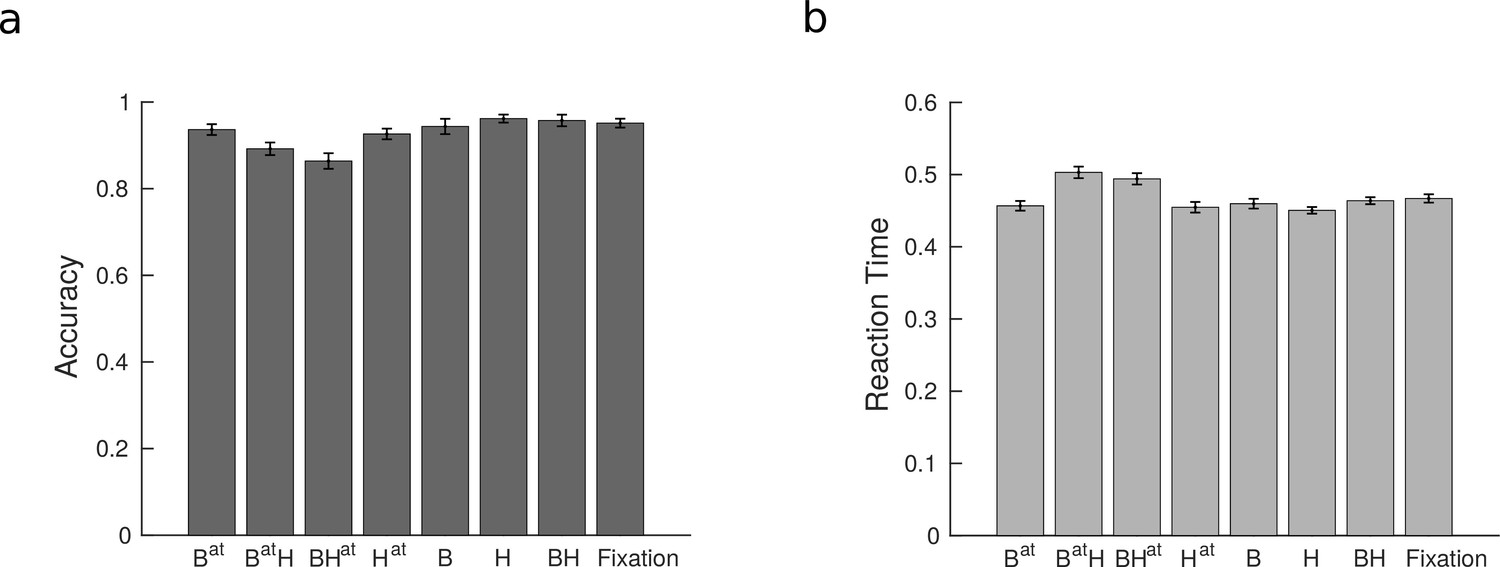
Behavioral performance of participants for the main experiment.
(a) Mean accuracy for each condition. Each condition’s label denotes the presented stimuli and the target of attention, with B and H denoting the presence of body and house stimuli, respectively, and the superscript and the superscript denoting the target of attention. Fixation denotes the fixation block with no stimulus. Error bars represent standard errors of the mean. N = 19 human participants. (b) Mean reaction time for each condition. Error bars represent standard errors of the mean. N = 19 human participants.
Figure 2 with 1 supplement
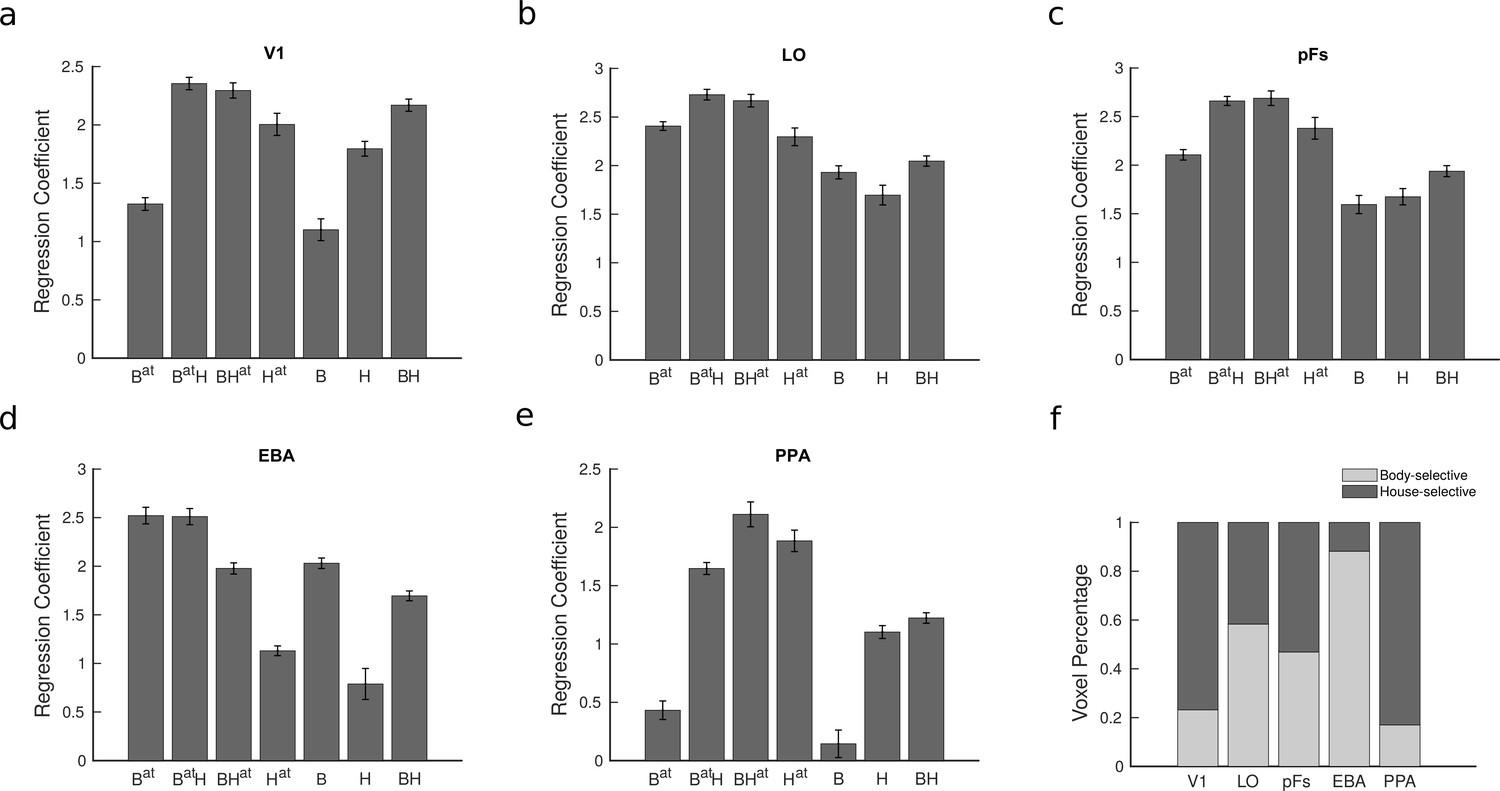
Average fMRI regression coefficients and voxel preference for the two categories in all regions of interest (ROIs).
(a–e) Average fMRI regression coefficients for each condition are illustrated in the five ROIs. Each condition’s label denotes the presented stimuli and the target of attention, with B and H, respectively, denoting the presence of body and house stimuli and the superscript denoting the target of attention. Therefore, the seven task conditions include Bat, BatH, BHat, Hat, B, H, and BH. For instance, the Hat condition refers to the isolated house condition with attention directed to houses, and the BH condition refers to the paired condition with attention directed to the fixation point color. Error bars represent standard errors of the mean for each condition, calculated across participants after removing the overall between-subject variance. N = 19 human participants. (f) The ratio of voxels preferring bodies and houses in each ROI. Both the regression coefficients and the voxel preference ratios were consistent across odd and even runs (see Figure 2—figure supplement 1 and Figure 2—figure supplement 1).
Figure 2—figure supplement 1
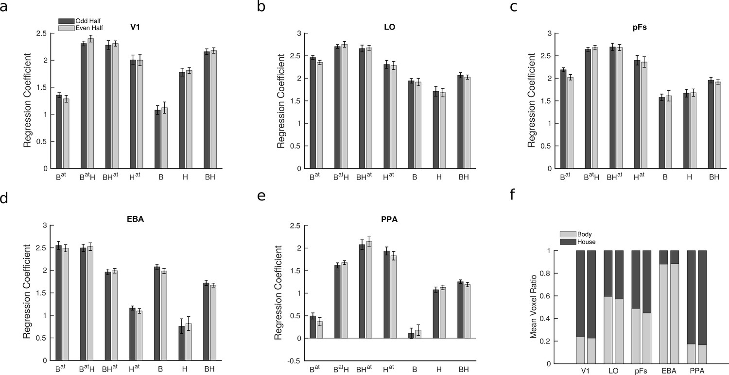
Average fMRI regression coefficients for each condition and voxel preference for the two categories in all ROIs, illustrated seperately for odd and even runs.
(a–e) Average fMRI regression coefficients for each condition in all regions of interest (ROIs), illustrated separately for odd and even runs. Dark gray bars represent the average regression coefficients across odd runs and light gray bars illustrate the average regression coefficients across even runs. Each condition’s label denotes the presented stimuli and the target of attention, with B and H, respectively, denoting the presence of body and house stimuli and the superscript denoting the target of attention. Error bars represent standard errors of the mean for each condition, calculated across participants after removing the overall between-subject variance. N = 19 human participants. (f) Voxel preference ratio in each region, plotted separately for odd (left bars) and even (right bars) runs. Light gray portions of the bars illustrate the mean ratio of body-selective voxels, and dark gray portions of the bars represent the ratio of house-selective voxels in each ROI.
Figure 3 with 2 supplements
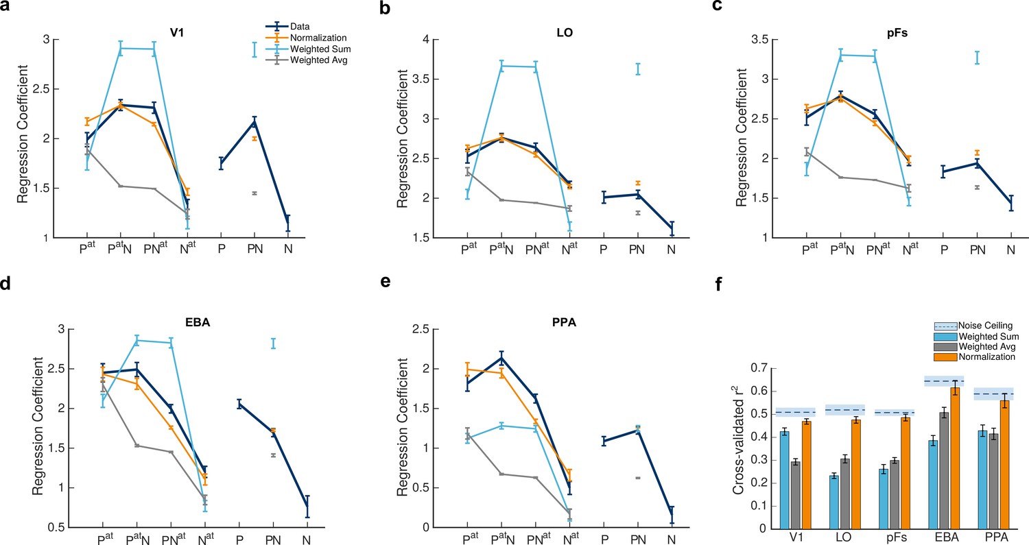
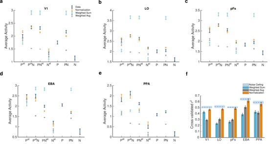
Divisive normalization explains voxel responses in different stimulus conditions.
(a–e) Average fMRI responses and model predictions in the five regions of interest. Navy lines represent average responses. Light blue, gray, and orange lines show the predictions of the weighted sum, the weighted average, and the normalization models, respectively. The x-axis labels represent the 7 task conditions, Pat, PatN, PNat, Nat, P, PN, N, with P and N denoting the presence of the preferred and null stimuli and the superscript denoting the attended category. For instance, P refers to the condition in which the unattended preferred stimulus was presented in isolation, and PatN refers to the paired condition with the attended preferred and unattended null stimuli. Error bars represent standard errors of the mean for each condition, calculated across participants after removing the overall between-subject variance. N = 19 human participants. (f) Mean explained variance, averaged over voxels in each region of interest for the 5 conditions predicted by the three models. Light blue, gray, and orange bars show the average variance explained by the weighted sum, the weighted average, and normalization models, respectively. Error bars represent the standard errors of the mean. N = 19 human participants. Dashed lines above each set of bars indicate the noise ceiling in each ROI, with the light blue shaded area representing the standard errors of the mean calculated across participants (see Figure 3—figure supplement 1 for an example illustration of how the goodness of fit was calculated for each voxel). As observed in the figure, the normalization model was a better fit for the data compared to the weighted sum (ps < 0.02) and the weighted average (ps < 0.0001) models. Simulation results demonstrate that this superiority is not related to the higher number of parameters or the nonlinearity of the normalization model (see Figure 3—figure supplement 2).
Figure 3—figure supplement 1
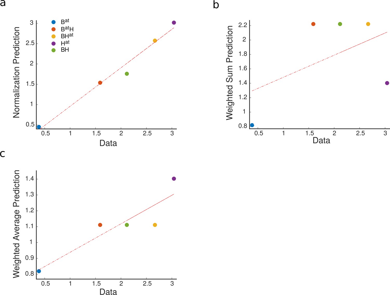
Calculation of model goodness of fit for an example voxel.
For each voxel, we calculated the correlation between voxel regression coefficients (data) and model predictions of the five modeled conditions. The r-squared of this correlation, averaged across all voxels in each regions of interest (ROI), represents the goodness of fit of the model. (a) The prediction of the normalization model versus the data for the five conditions. (b) The prediction of the weighted sum model versus the data (c) The prediction of the weighted average model versus the data. For the example voxel illustrated in this figure, we observe that the normalization model made closer predictions of the data across the five conditions. For comparison, the weighted average model made close predictions for some conditions (Bat and BH), but its predictions of the remaining conditions were not as close.
Figure 3—figure supplement 2
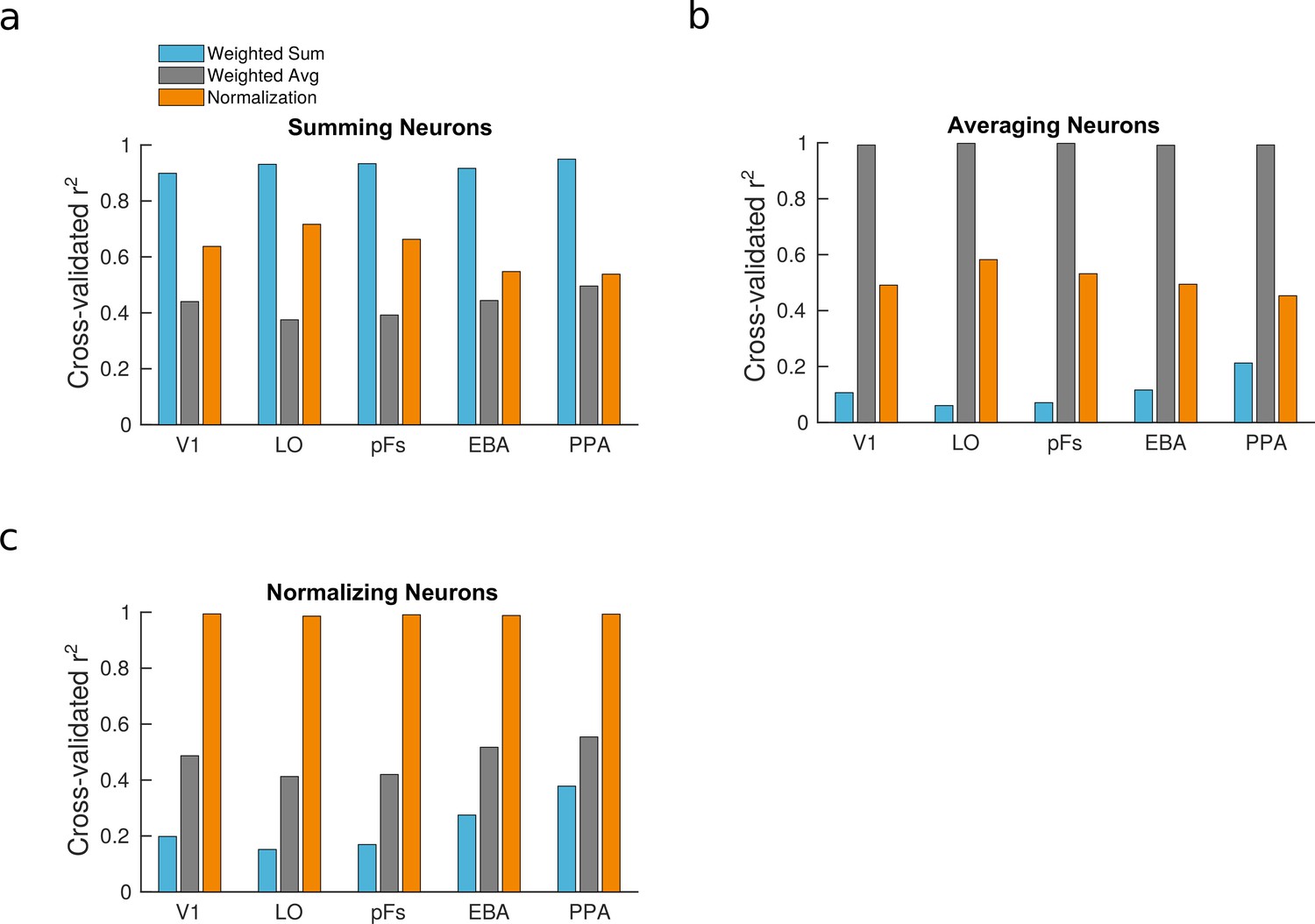
Goodness of fit of the three models for the simulated neural populations.
(a) Population of summing neurons. The weighted sum model provides the best fit for a population of summing neurons. (b) Population of averaging neurons. The weighted average model is the best fit for averaging neurons. (c) Population of normalizing neurons. The normalization model is the best model for predicting the responses of normalizing neurons.
Figure 4
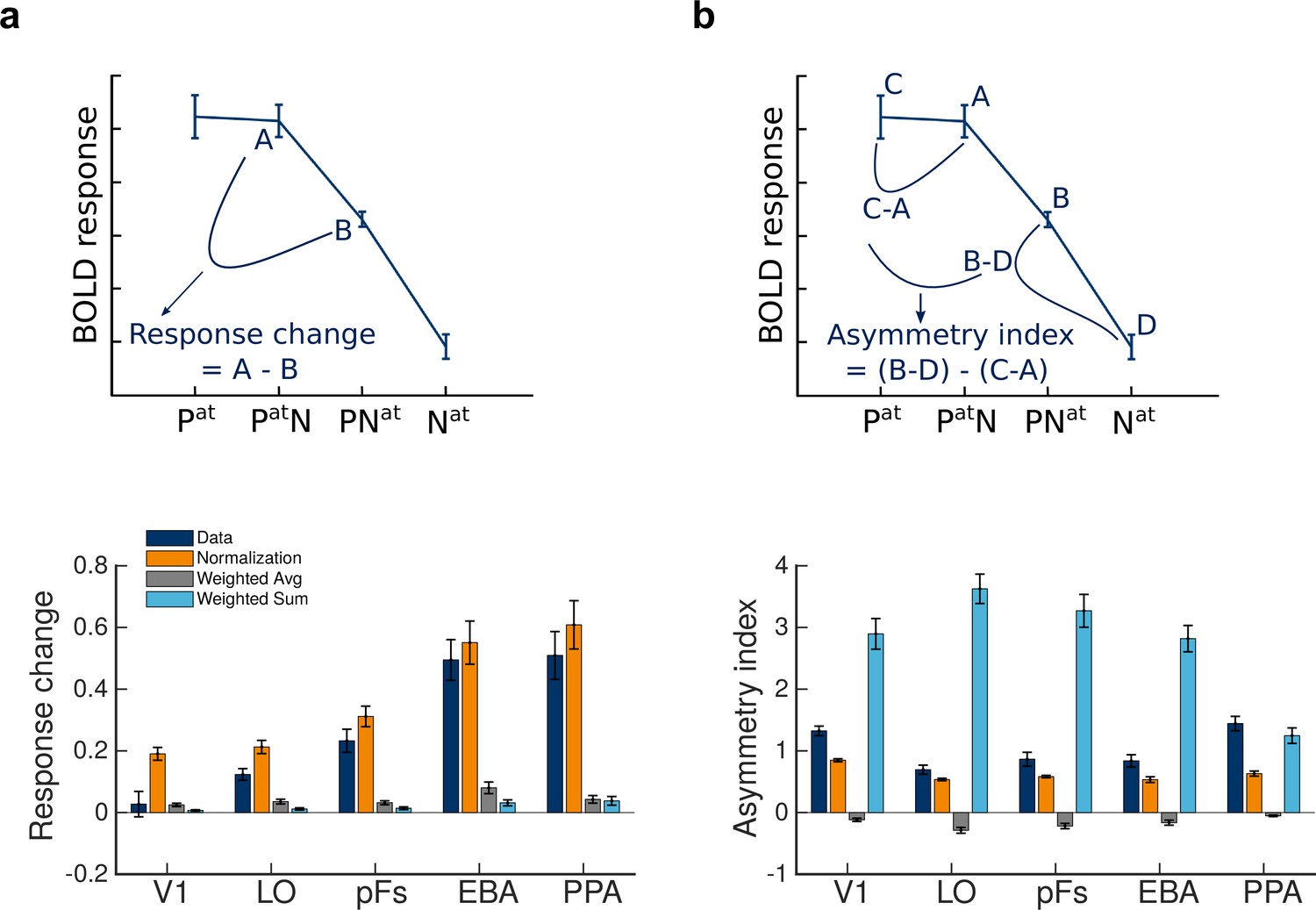
Normalization accounts for the observed effects of attention.
(a) Top: Change in BOLD response when attention shifts from the preferred to the null stimulus in the presence of two stimuli, illustrated here for extrastriate body area (EBA). Bottom: The observed response change and the corresponding amount predicted by different models in different regions, calculated as illustrated in plot A. Error bars represent the standard errors of the mean. N = 19 human participants. (b) Top: The observed asymmetry in attentional modulation for attending to the preferred versus the null stimulus, depicted for EBA. Bottom: The observed and predicted asymmetries in attentional modulation in different regions, calculated as illustrated in plot B. Error bars represent the standard errors of the mean. N = 19 human participants.
Figure 5
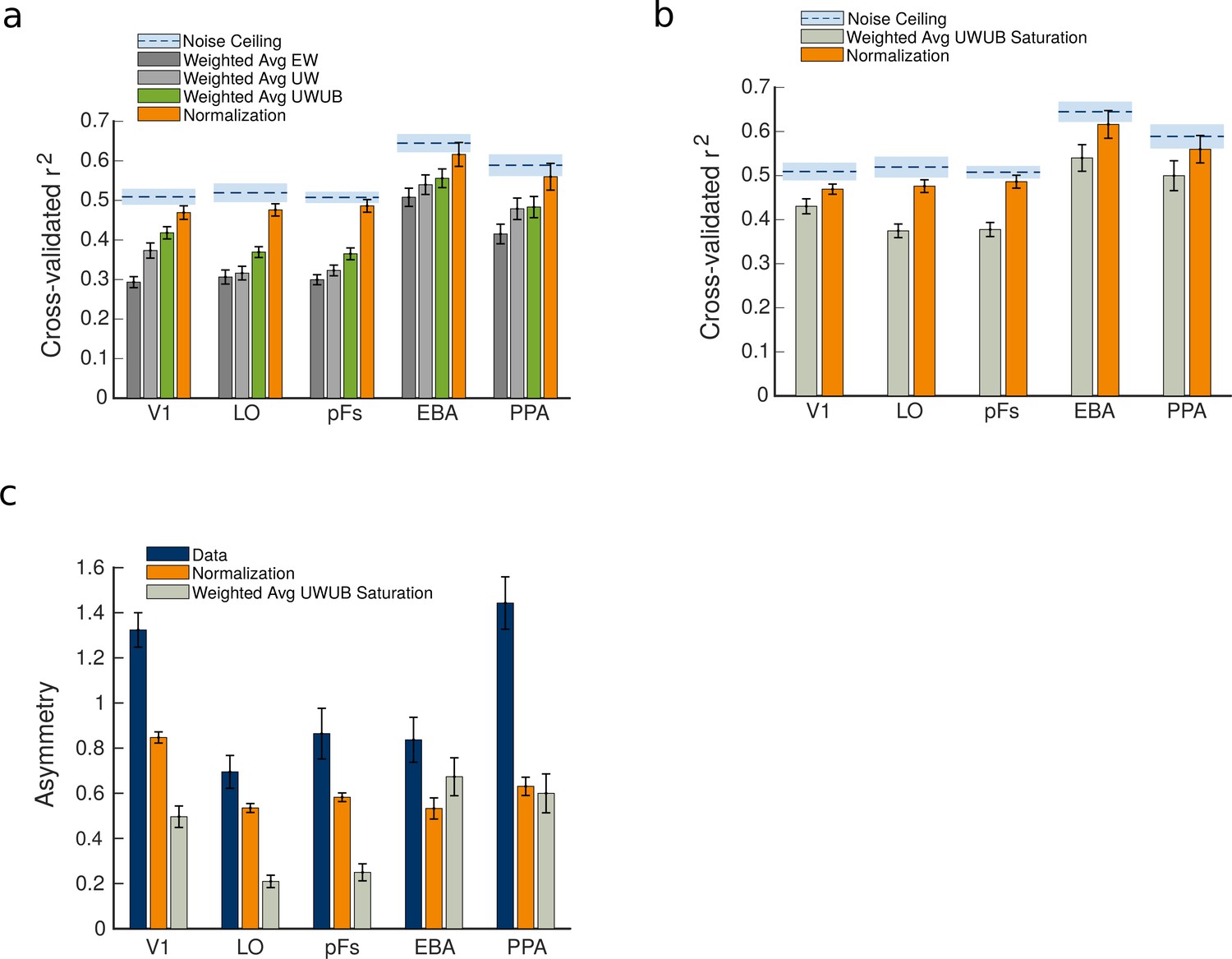
Comparison between the weighted average model variants and the normalization model predictions.
(a) Comparison of the goodness of fit for weighted average variants and the normalization model. (b) The goodness of fit of the normalization model compared to the weighted average unequal weights and unequal betas (UWUB) saturation variant. (c) The asymmetry index was calculated for the data, compared to the predictions of the normalization model and the weighted average UWUB saturation model. Error bars represent the standard errors of the mean, calculated across N = 19 human participants.
Author response image 1
Author response image 2
Additional files
-
Supplementary file 1
Voxel preference consistency percentage across odd and even runs.
- https://cdn.elifesciences.org/articles/75726/elife-75726-supp1-v4.xlsx
-
Supplementary file 2
Difference between the AIC values of the fits of the three models.
- https://cdn.elifesciences.org/articles/75726/elife-75726-supp2-v4.xlsx
-
Supplementary file 3
Estimated parameters of the weighted sum model.
- https://cdn.elifesciences.org/articles/75726/elife-75726-supp3-v4.xlsx
-
Supplementary file 4
Estimated parameters of the weighted average model.
- https://cdn.elifesciences.org/articles/75726/elife-75726-supp4-v4.xlsx
-
Supplementary file 5
Estimated parameters of the normalization model.
- https://cdn.elifesciences.org/articles/75726/elife-75726-supp5-v4.xlsx
-
Supplementary file 6
Estimated parameters of the weighted average UW model.
- https://cdn.elifesciences.org/articles/75726/elife-75726-supp6-v4.xlsx
-
Supplementary file 7
Estimated parameters of the weighted average UWUB model.
- https://cdn.elifesciences.org/articles/75726/elife-75726-supp7-v4.xlsx
-
Supplementary file 8
Estimated parameters of the weighted average UWUB saturation model.
- https://cdn.elifesciences.org/articles/75726/elife-75726-supp8-v4.xlsx
-
MDAR checklist
- https://cdn.elifesciences.org/articles/75726/elife-75726-mdarchecklist1-v4.pdf
Download links
A two-part list of links to download the article, or parts of the article, in various formats.
Downloads (link to download the article as PDF)
Open citations (links to open the citations from this article in various online reference manager services)
Cite this article (links to download the citations from this article in formats compatible with various reference manager tools)
The normalization model predicts responses in the human visual cortex during object-based attention
eLife 12:e75726.
https://doi.org/10.7554/eLife.75726


