Quantitative mapping of keratin networks in 3D
- Institute of Molecular and Cellular Anatomy, RWTH Aachen University, Germany
- Interdisciplinary Centre for Clinical Research, RWTH Aachen University, Germany
- Department of Computer Science, RWTH Aachen University, Germany
- Institute of Imaging and Computer Vision, RWTH Aachen University, Germany
- Visual Computing Institute, RWTH Aachen University, Germany
- DWI – Leibniz-Institute for Interactive Materials, Germany
Figures
Figure 1 with 3 supplements
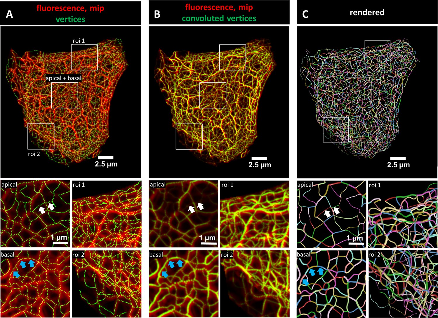
Evaluation of 3D keratin filament network segmentation.
The pictures show three different numerical representations of the same fluorescence data set detecting the keratin filament network in an MDCK cell expressing fluorescently labeled keratin 8. The cell is part of a confluent monolayer and the fluorescence of the single cell shown was manually excised from an image stack consisting of 32 slices (voxel size: xy = 66 nm, z = 182 nm). This cropped fluorescence was used to calculate the vertex positions and intensity of all keratin filaments. (A) The top picture shows an overlay of the recorded fluorescence in red as a maximum intensity projection (mip) and the corresponding calculated xy positions of vertices of all segments as green dots. The enlargements below (corresponding regions demarcated by boxes) show maximum intensity projections of focal planes above and below the nucleus (apical and basal) at left and two regions of interest (roi 1, roi 2) depicting maximum intensity projections of all focal planes in the cell periphery. (B) Presents an overlay of the keratin fluorescence and corresponding vertices that were plotted in 3D with a diameter relative to their brightness and were subsequently subjected to 3D Gaussian blurring to simulate the microscope’s blur. The enlargements correspond to those shown at left in (A) presenting the same regions of interest and focal planes. The top panel of Video 1 presents an animated comparison of the fluorescence recording, segmentation and overlay in each focal plane. (C) Depicts a cinematic rendering of segments. Each calculated segment is rendered in 3D with a thickness corresponding to the brightness of the original filament. The color-coding helps to identify and distinguish individual segments. The regions of interest correspond to the same single planes as those shown in (A). White arrows demarcate thin filaments, blue arrows thick filaments.
Figure 1—figure supplement 1
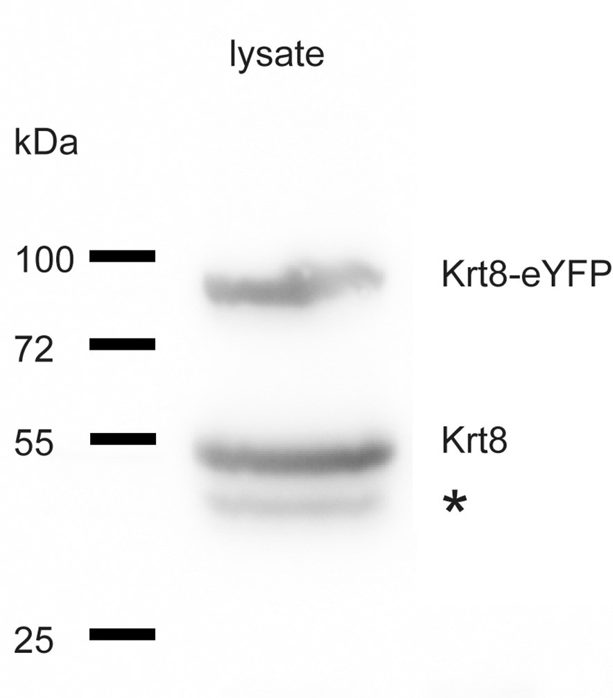
Immunoblot of a total lysate of a transgenic MDCK cell clone detecting endogenous wild-type keratin 8 (Krt8) and eYFP-tagged keratin 8 (Krt8-eYFP).
Cells were lysed in 40 mM Tris-Cl (pH), suspended in Laemmli buffer at 4 °C and separated by SDS-polyacrylamide gel electrophoresis. After transfer onto polyvinylidene fluoride Immobilon-P membrane (Millipore), keratin 8 epitopes were detected with a rat monoclonal anti-keratin 8 (TROMA-1) hybridoma cell supernatant (Developmental Studies Hybridoma Bank) and visualized with the help of secondary antibodies and the ECL system. The position and molecular weight of co-electrophoresed markers are indicated at left, the star denotes an immunoreactive band of unknown identity.
Figure 1—figure supplement 2
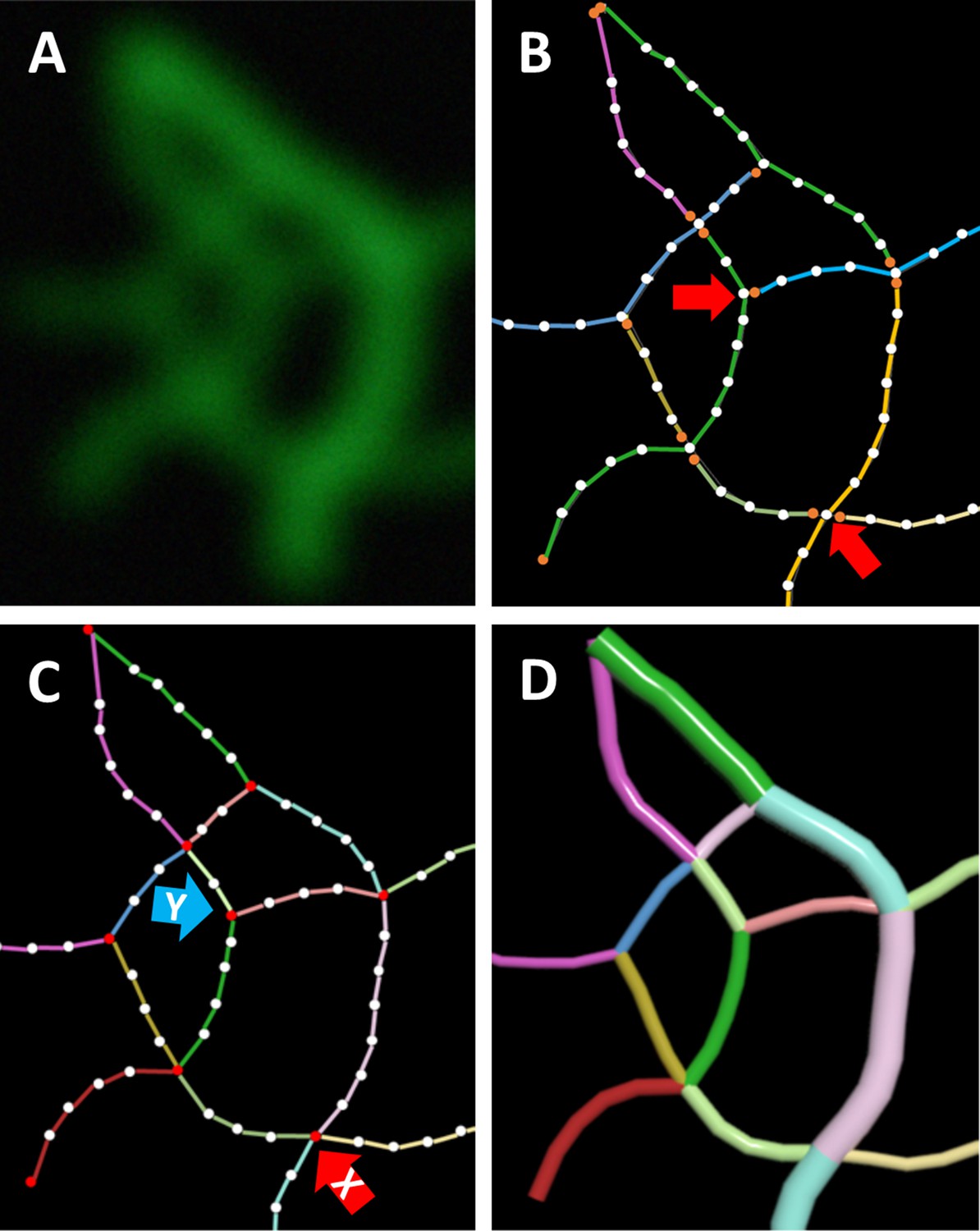
Exemplary representation of major steps in the workflow.
All data are in 3D. (A) Maximum intensity projection of a small region of interest taken from an airyscan image of fluorescently labeled keratin filaments. (B) ‘Snakes’ prepared by TSOAX segmentation. White dots represent vertices and orange dots represent start and end vertices of ‘snakes’. Colored lines distinguish individual ‘snakes’. Note that ‘snakes’ are not well defined since not all ‘snakes’ have an end at intersections (red arrows). Therefore, the start and end points of snakes are not defined and snakes may span over several intersections. (C) In the final segmentation, segments (colored lines) and nodes (red dots) are defined. No intersections of segments exist. Each segment has a start and end point ( = node), and segments are connected by nodes. Y-shaped (blue arrow) or X-shaped (red arrow) branchings occur. (D) The cinematic rendering shows segments as tubes. Thickness represents mean brightness.
Figure 1—figure supplement 3
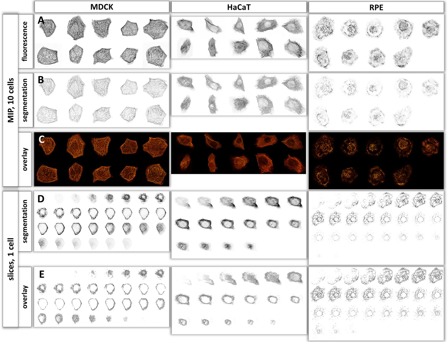
Validation of segmentation.
(A) Maximum intensity projections of airyscan recordings of 10 cells each (left, MDCK; middle, HaCaT; right, RPE). (B) The pictures show the xy-position and brightness of segment vertices after 3D-Gaussian blurring. The resulting convolutions mimic those of microscopic imaging. (C) The merged images were prepared by overlay of the first and second row above to compare original imaging data with segmentation. (D) The picture shows all digital representations prepared from focal planes of airyscan image stacks of single cells. The xy-position of all segments is plotted in their corresponding slice position. Corresponding Video 1 shows an animated version of the data.
Figure 2 with 1 supplement
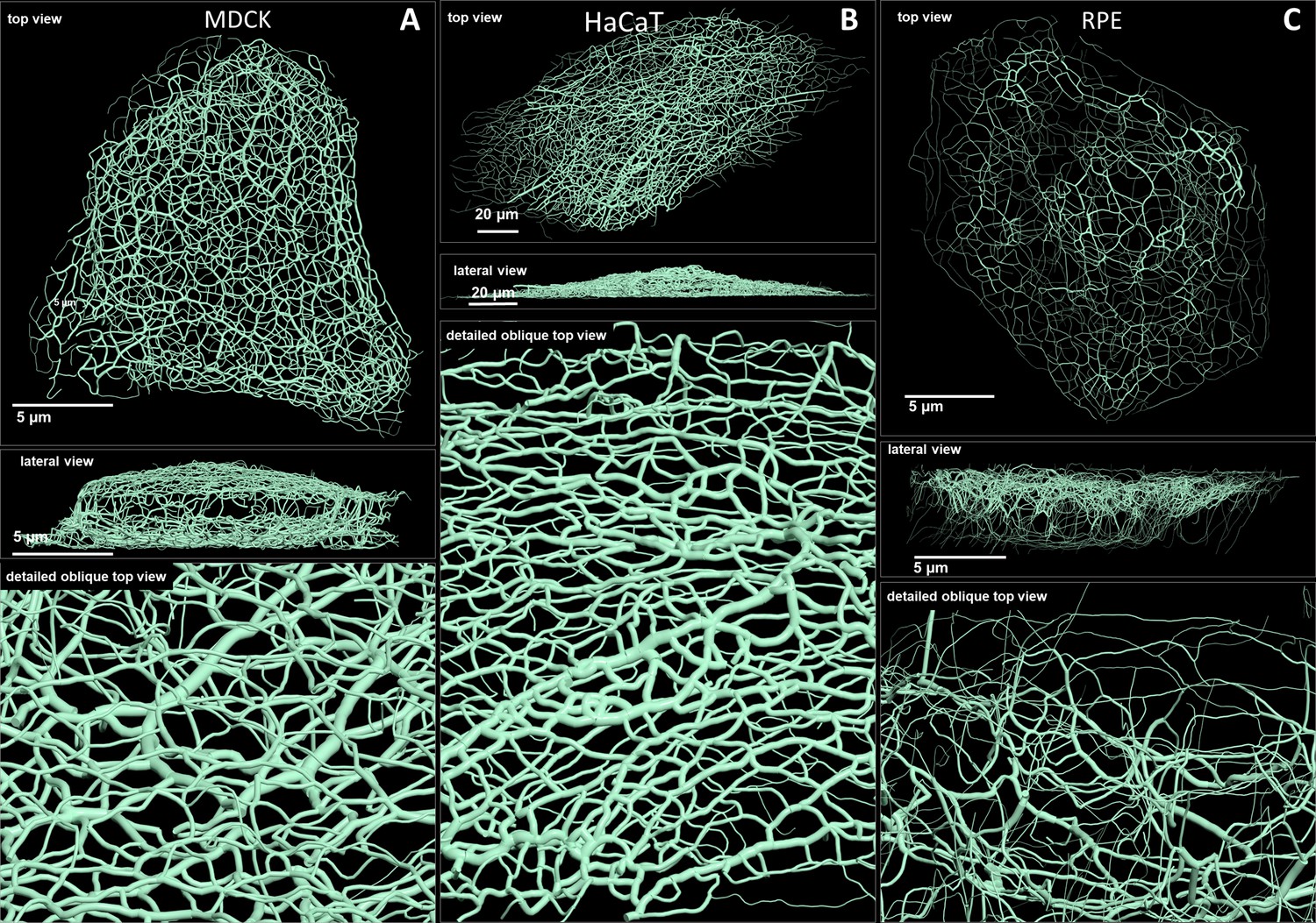
Comparison of 3D cinematic rendering of keratin filaments in three different epithelial cell types.
The position and intensity of fluorescence recordings were transferred into a numerical 3D-representation of individual segments. The thickness of the segments corresponds to the fluorescence brightness in the original data. (A) Shows cinematic rendering of keratin filaments of an MDCK cell expressing fluorescently labeled keratin 8. Video 2 presents the 3D-animation of the cell. (B) Depicts the cinematic rendering of keratin filaments in a HaCaT keratinocyte expressing fluorescently labeled keratin 5 (animation in Video 3). (C) Illustrates cinematic rendering of keratin filaments in a single RPE cell of a homozygous keratin 8-YFP knock-in mouse (animation in Video 4).
Figure 2—figure supplement 1
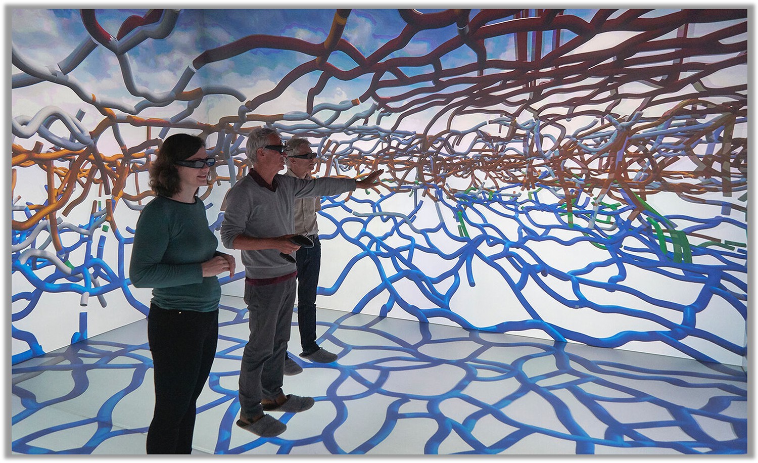
Visual inspection of the keratin network of a single cell in a virtual reality environment.
The viewer can move freely within the network which appears to her/him as a true 3D stereoscopic structure. Classification of segments is done interactively in this environment by color coding.
Figure 3

Mapping of keratin filament brightness in MDCK, HaCaT, and RPE cells.
(A–C) The histograms display the distribution of relative segment brightness for each cell type. The maximum brightness was normalized to 100 in all cases. For each segment, the mean brightness was calculated and the determined brightness levels of all segments in 10 cells were pooled for each diagram. (D–F) The maps depict the segment brightness in a representative MDCK (left), HaCaT (middle) and RPE (right) cell (top panel; enlarged boxed area in bottom panel). The color code represents relative brightness.
Figure 4 with 1 supplement
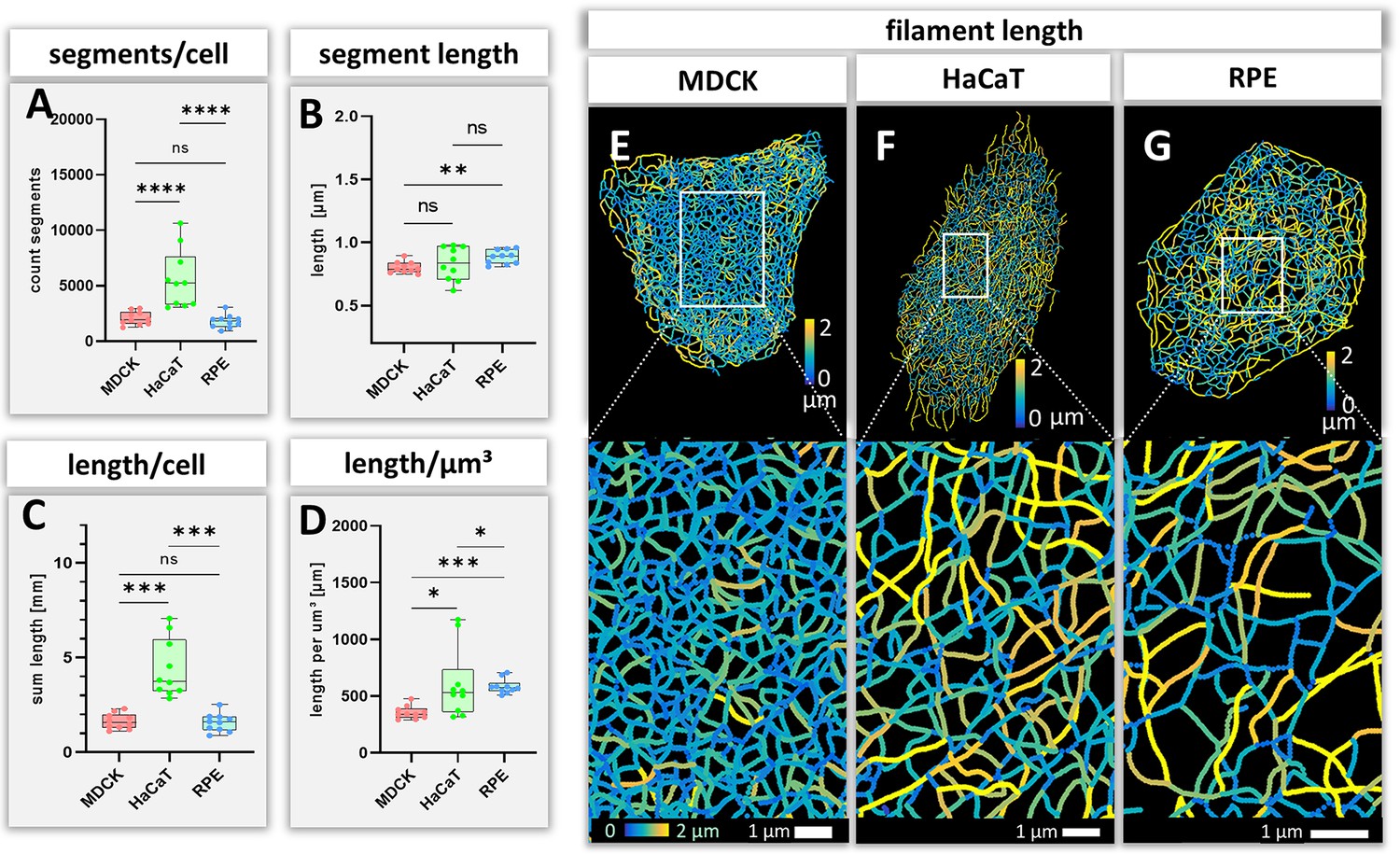
Measurements of keratin filaments in MDCK, HaCaT and RPE cells.
(A–D) The whisker box plots depict the number of segments per cell (A), the mean segment length (B), the entire length of the keratin filament network within a single cell (C) and the filament length per µm³ (D). Ten cells were analyzed for each cell type. (E–G) show color-coded keratin filament segment lengths for each cell type. The top panel presents the results for entire cells, the bottom panel the results for the boxed areas at higher magnification.
Figure 4—figure supplement 1

Boxplots of cell volumes estimated from fluorescence image stacks (A) and calculated virtual persistence length of segments (B) in MDCK, HaCaT and RPE cells.
Figure 5
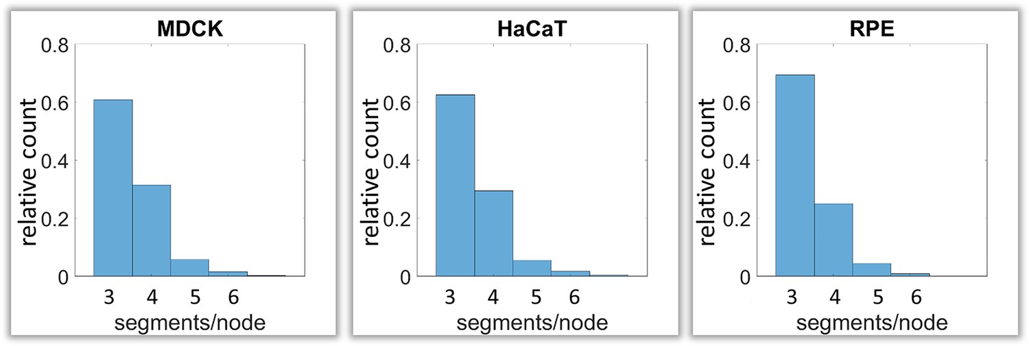
Calculation of keratin filament node types based on segment/node ratios in MDCK, HaCaT and RPE cells.
A segment/node ratio of 3 refers to Y-shaped branching, a ratio of 4 to X-shaped branchings. Higher values refer to star-like branchings. The histograms depict the relative distribution of node types.
Figure 6
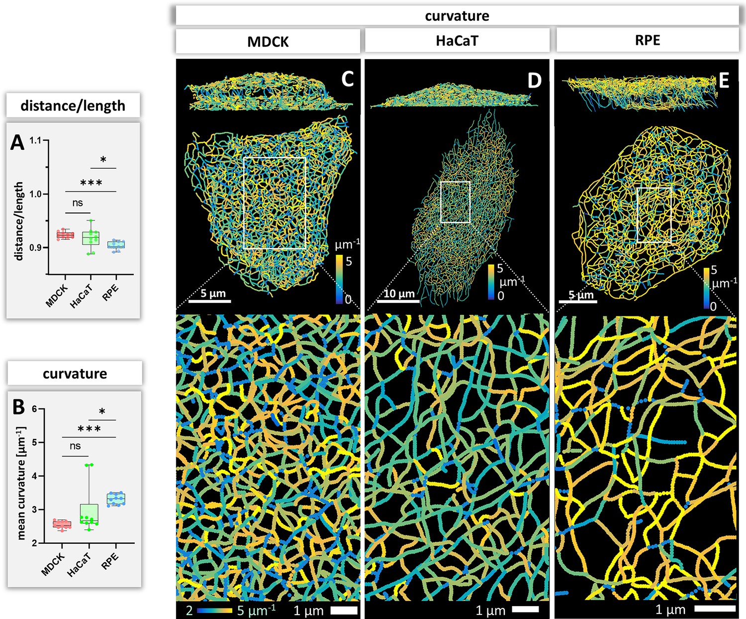
Measurements of keratin filament segment bending in MDCK, HaCaT, and RPE cells.
(A) The whisker box plot shows the distance/length ratio of keratin segments. (B) The curvature of keratin filaments in the three cell types is shown as a whisker box plot. (C–E) Color-coded representation of the keratin network depicting the curvature of keratin filament segments in entire cells (top) and selected regions of interest (boxed areas) at higher magnification (bottom).
Figure 7 with 2 supplements

Orientation of keratin filament segments in MDCK, HaCaT, and RPE cells.
(A–C) The histograms show the normalized distribution of azimuth ( = horizontal orientation) of keratin filament segments in single cells. Since the start and end points are interchangeable, the histogram is restricted to 180 degrees. The horizontal line represents the expected histogram levels, if all angles were equally distributed. (D–F) The histograms show the elevation ( = vertical orientation) of keratin filament segments. The horizontal line demarcates the expected histogram values, if elevation of keratin filament segments would be uniform. (G, H) Whisker box plots depicting the deviation of segment orientations from uniform unbiased distributions. The differences in azimuth (G) and elevation (H) were calculated for 10 MDCK, 10 HaCaT and 10 RPE cells. (I–L) The color-coded maps depict the azimuth of segments in entire cells (top; MDCK, left; HaCaT, middle; RPE, right) and selected regions of interest (boxed areas; bottom).
Figure 7—figure supplement 1
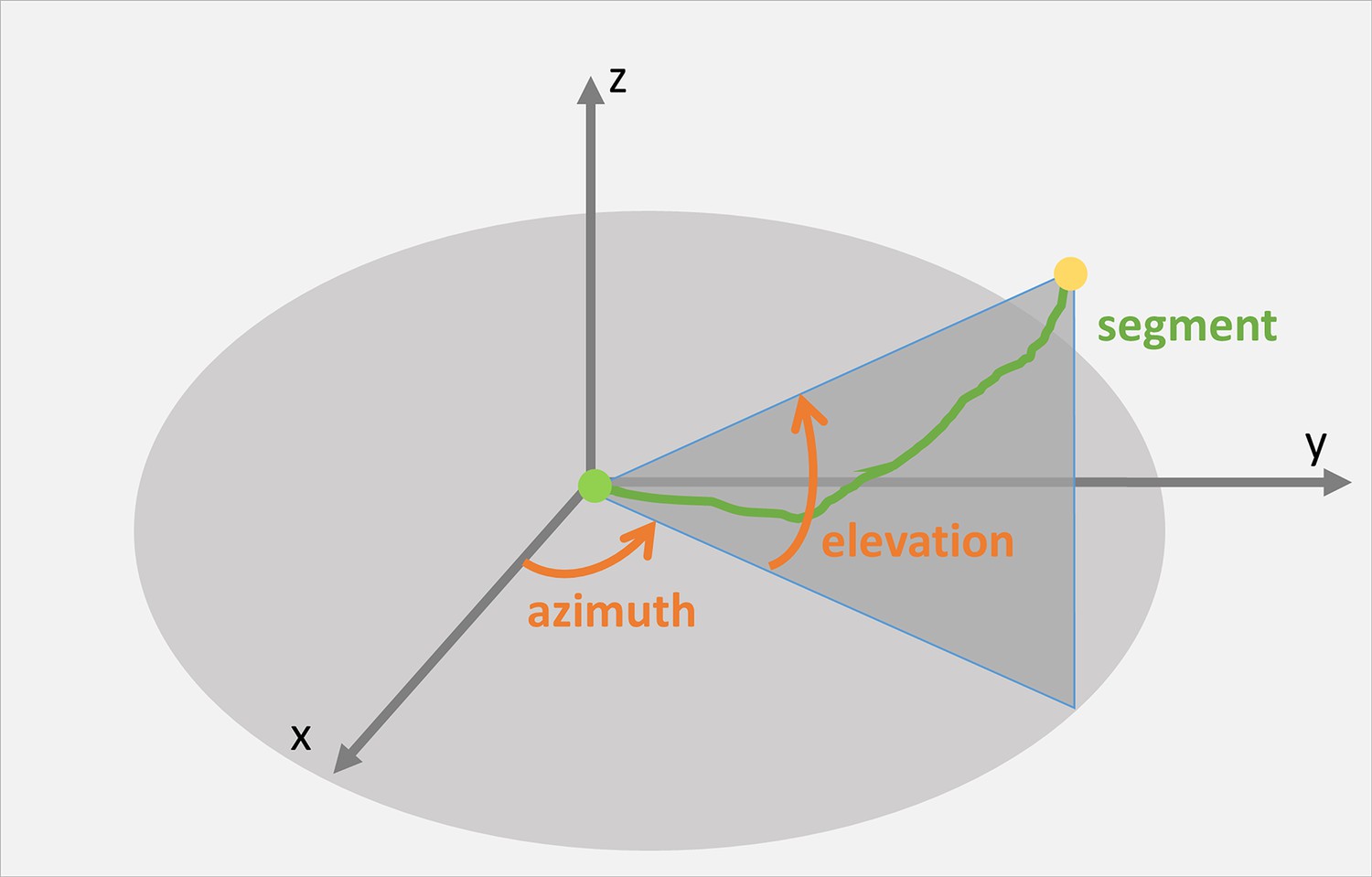
Schematic illustration of keratin filament segment (green) orientation in 3D space.
The orientation of a given segment between start point (green dot) and end point (yellow dot) is calculated as the angles of azimuth and elevation.
Figure 7—figure supplement 2
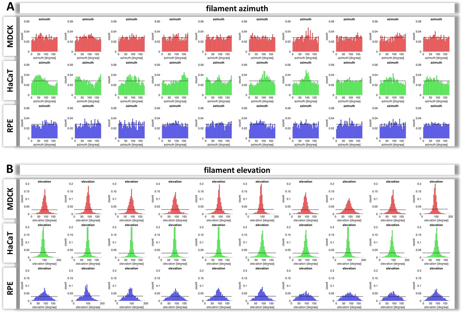
Histograms of keratin filament orientation in MDCK, HaCaT, and RPE cells.
(A) The normalized histograms show the normalized distribution of azimuth ( = horizontal orientation) of keratin filament segments in 10 MDCK, HaCaT, and RPE cells, respectively. Since the segments have no defined start and end point, the histograms are restricted to 180 degree. The horizontal line represents the value, if all angles were uniformly distributed. (B) The normalized histograms show the elevation ( = vertical orientation) of keratin filament segments in 10 MDCK, HaCaT, and RPE cells. The horizontal line delineates the value, if all angles were uniformly distributed.
Figure 8
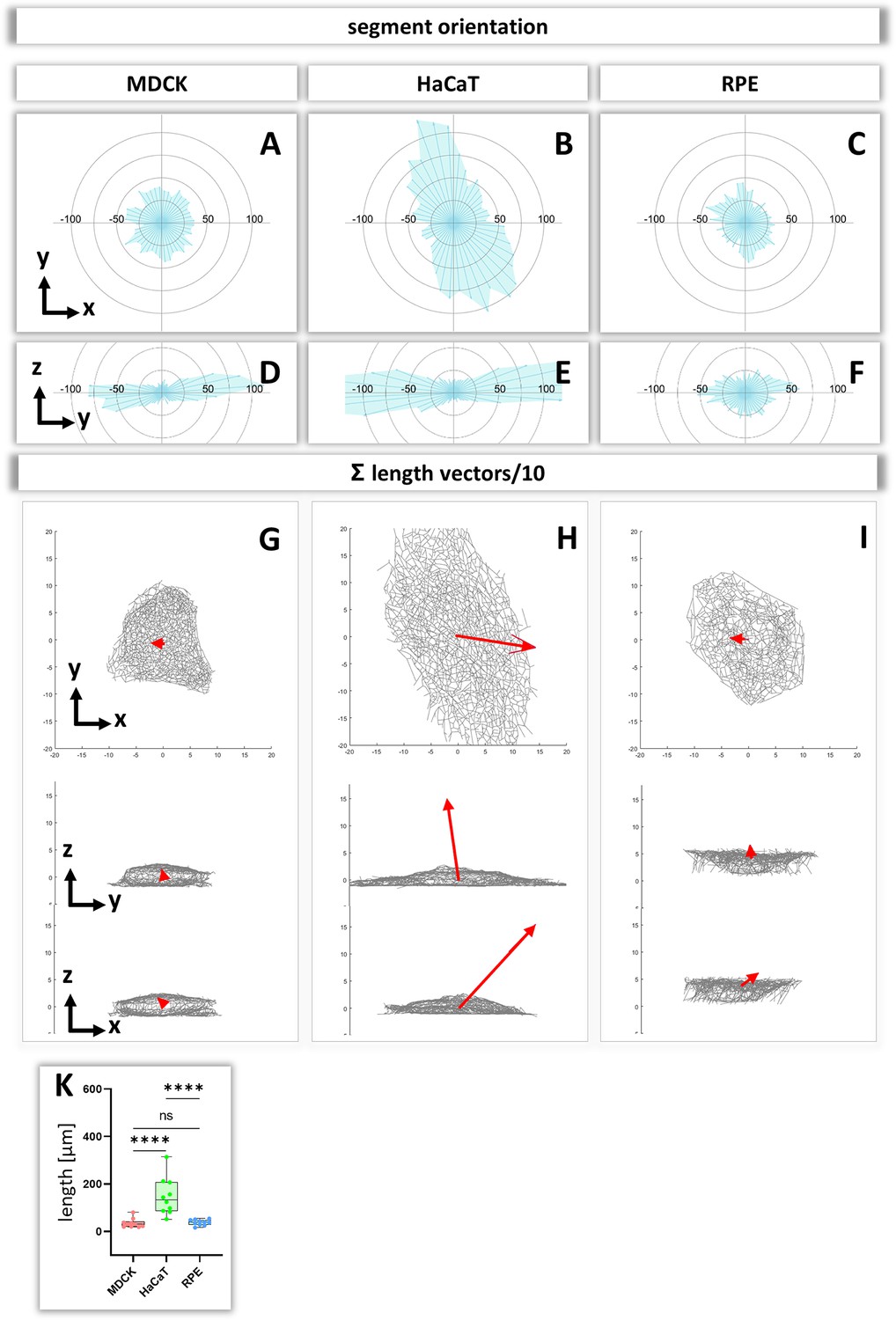
Analysis of segment orientation in MDCK, HaCaT, and RPE cells.
(A–F) The blue polygons represent radial histograms of the orientation of keratin filament segments in relation to the cell center of single cells. Horizontal orientation (A–C) and the vertical orientation (D–F) are shown. Each keratin segment in each cell was moved to the cell center and vectors pointing in the same directions were added. Thus, the longer the blue lines are, the more vectors point in that direction. (G–I) The red arrows represent the sum vectors of the direction and length of all segments in each cell. (K) Whisker box plots depicting the length of the main vectors in all three cell types.
Figure 9
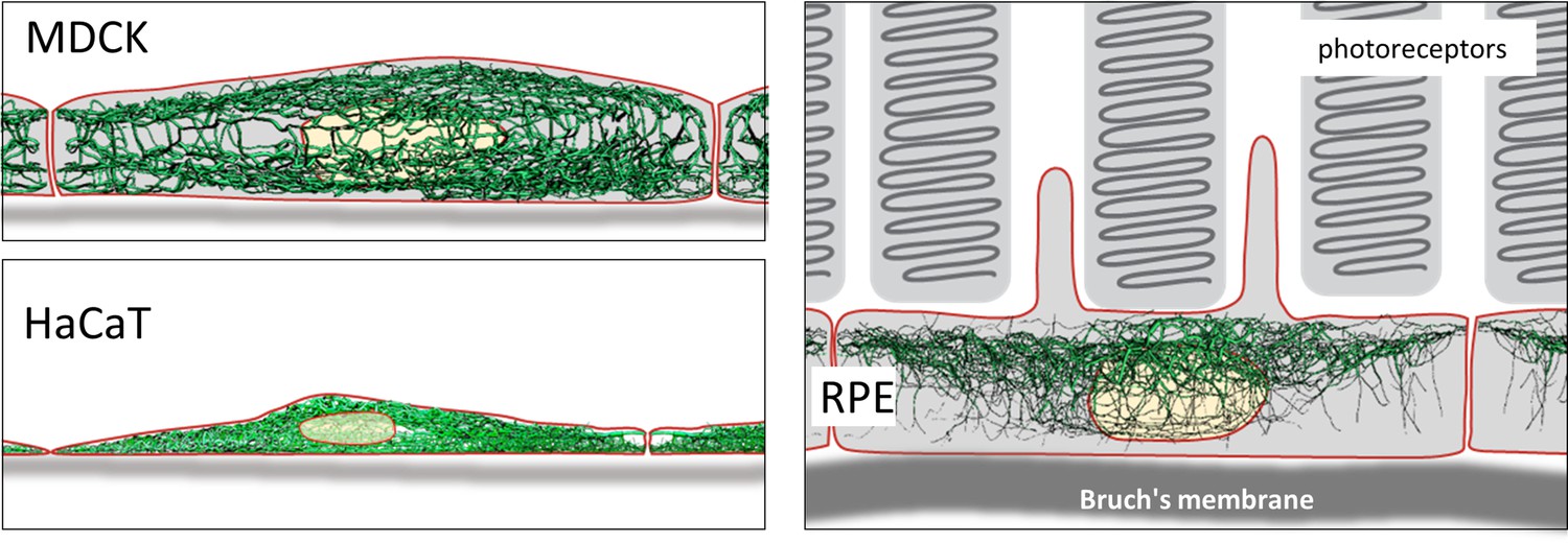
Schematic drawing of the reconstructed keratin network in the three cell types investigated.
Author response image 1
Videos
Video 1
Validation of keratin filament segmentation in an MDCK, HaCat and RPE cell.
The animation shows the original fluorescence image stacks (left), the segmented data including the associated brightness (middle) and the overlays of both (right).
Video 2
Cinematic rendering of the reconstructed keratin filament network of an MDCK cell growing in a confluent monolayer.
The tubes represent keratin bundles with different thickness. At the beginning of the video, the segments are randomly color-coded.
Video 3
Cinematic rendering of the numerical reconstructed keratin network of a HaCaT cell growing in a confluent monolayer.
The tubes represent keratin bundles with different thickness. At the beginning of the video, the segments are randomly color-coded.
Video 4
Cinematic rendering of the numerical reconstructed keratin network of an RPE cell.
The tubes represent keratin bundles with different thickness. At the beginning of the video, the segments are randomly color-coded.
Additional files
Download links
A two-part list of links to download the article, or parts of the article, in various formats.
Downloads (link to download the article as PDF)
Open citations (links to open the citations from this article in various online reference manager services)
Cite this article (links to download the citations from this article in formats compatible with various reference manager tools)
Quantitative mapping of keratin networks in 3D
eLife 11:e75894.
https://doi.org/10.7554/eLife.75894


