Complex fitness landscape shapes variation in a hyperpolymorphic species
Figures

The efficiency of epistatic selection in populations with different levels of genetic diversity.
(A–C) LD in natural populations for SNPs with MAF >0.05. (A) USA population of S. commune, (B) Zambian population of D. melanogaster, (C) African superpopulation of H. sapiens. Filled areas in (A)-(C) indicate SE of LD calculated for each chromosome or scaffold separately. (D–F) A hyperpolymorphic population (D) may occupy a sizeable chunk of a complex fitness landscape, leading to pervasive positive epistasis, while variation within less polymorphic populations (E and F) is confined to smaller, and approximately linear, portions of the landscape, so that no strong epistasis and LD can emerge. The area of the landscape covered by the population is shown in green.
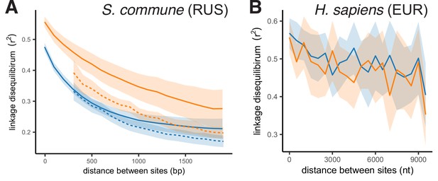
The efficiency of epistatic selection in populations with different levels of genetic diversity.
LD between nonsynonymous SNPs is shown in orange, and LD between synonymous SNPs is shown in blue. (A) Russian population of S. commune, (B) European super-population of H. sapiens. Solid lines indicate LD between pairs of SNPs located within the same gene; dashed lines correspond to pairs of SNPs located in different genes. Only SNPs with minor allele frequency > 0.05 are analysed. Filled areas indicate SE of LD calculated for each chromosome (for human) or scaffold (for S. commune) separately.
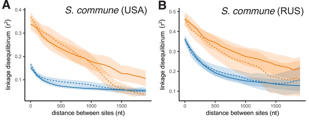
Linkage disequilibrium within and between exons in S. commune.
LD between nonsynonymous SNPs is shown in orange, and LD between synonymous SNPs is shown in blue. Solid lines indicate LD between pairs of SNPs located within the same exon of the gene; dashed lines correspond to pairs of SNPs located in different exons of the gene. (A) USA population of S. commune, (B) RUS population of S. commune. Only SNPs with minor allele frequency > 0.05 are analysed. Filled areas indicate SE of LD calculated for each scaffold separately.
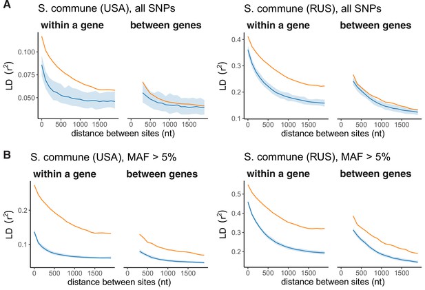
Comparison of LDnonsyn and LDsyn in S. commune populations with exact matching of both MAFs and distance.
For each possible minor allele count and nucleotide distance, the number of corresponding pairs of nonsynonymous variants and LDnonsyn between them is calculated. Then, the same number of synonymous variants on the same nucleotide distance and with the same minor allele count is randomly chosen to calculate LDsyn. Subsampling is performed for 100 times. Filled areas show 95% intervals of LDsyn in the subsamples. (A) All SNPs, (B) SNPs with MAF >0.05.
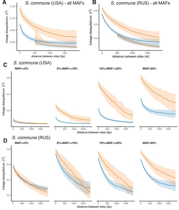
LD between SNPs with different MAF in S. commune.
LD between nonsynonymous SNPs is shown in orange, and LD between synonymous SNPs is shown in blue. Filled areas indicate SE of LD calculated for each scaffold separately. (A, B) LD between all pairs of SNPs pooled together. Solid lines indicate LD between pairs of SNPs located within the same gene; dashed lines correspond to pairs of SNPs located in different genes. (C, D) Pairs of SNPs split by MAF.
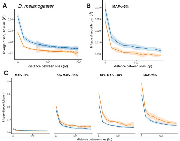
LD between SNPs with different MAF in D. melanogaster.
LD between nonsynonymous SNPs is shown in orange, and LD between synonymous SNPs is shown in blue. Filled areas indicate SE of LD calculated for each chromosome separately. (A) LD between all pairs of SNPs pooled together. Solid lines indicate LD between pairs of SNPs located within the same gene; dashed lines correspond to pairs of SNPs located in different genes. (B) Pairs of SNPs with MAF <0.05 (large scale). (C) Pairs of SNPs split by MAF.
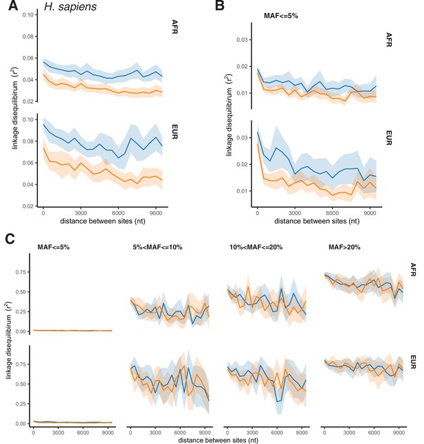
LD between SNPs with different MAF in H. sapiens.
LD between nonsynonymous SNPs is shown in orange, and LD between synonymous SNPs is shown in blue. Filled areas indicate SE of LD calculated for each chromosome separately. (A) LD between all pairs of SNPs pooled together. Solid lines indicate LD between pairs of SNPs located within the same gene; dashed lines correspond to pairs of SNPs located in different genes. (B) Pairs of SNPs with MAF <0.05 (large scale). (C) Pairs of SNPs split by MAF.
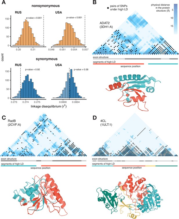
Excessive LD between physically interacting protein sites.
(A) Within pairs of SNPs that correspond to pairs of amino acids that are colocalized within 10 Å in the protein structure, the LD is elevated between nonsynonymous, but not between synonymous, variants. Dashed lines show the average LD between colocalized sites. Permutations were performed by randomly sampling pairs of non-interacting SNPs while controlling for genetic distance between them, measured in amino acids; pairs of SNPs closer than 5 aa were excluded. (B–D) Examples of proteins with LD patterns matching their three-dimensional structures. Heatmaps show the physical distance between pairs of sites in the protein structure; only positions carrying biallelic SNPs are shown. Black dots correspond to pairs of sites with high LD (>0.9 quantile for the gene). Dashed lines in (c) structure show high LD between physically close SNPs from different segments of high LD. In these examples, LD is calculated in the Russian population of S. commune.
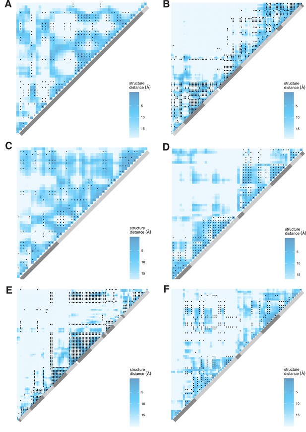
Examples of proteins with LD patterns matching the three-dimensional structure in the RUS population of S. commune.
Heatmaps show the physical distance between pairs of sites in the protein structure; only positions carrying biallelic SNPs are shown. Black dots correspond to pairs of sites with high LD (>0.9 quantile for the gene). Grey regions indicate the exon structure of the genes. (A) cog1523 (5Y1B:A); (B) cog2779 (1SXJ:B); (C) cog5375 (1RGI:G); (D), cog5725 (1TA3:B); (E) cog18092 (4QJY:A); (F) cog7878 (4TYW:A). LD statistics and p-values for each gene are listed in Appendix 3—table 1.
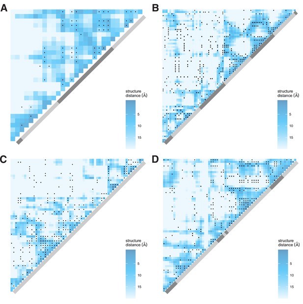
Examples of proteins with LD patterns matching the three-dimensional structure in the USA population of S. commune.
Heatmaps show the physical distance between pairs of sites in the protein structure; only positions carrying biallelic SNPs are shown. Black dots correspond to pairs of sites with high LD (>0.9 quantile for the gene). Grey regions indicate the exon structure of the genes. (A) cog1536 (6AHR:E); (B) cog5725 (1TA3:B); (C) cog8253 (6F87:A); (D) cog9241 (1YCD:A). LD statistics and p-values for each gene are listed in Appendix 3—table 1.
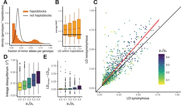
Patterns of linkage disequilibrium in the USA population of S. commune.
(A) Distribution of the fraction of polymorphic sites that carry minor alleles in a genotype within haploblocks. Black line shows the distribution of fraction of minor alleles in genotypes in non-haploblock regions. (B) Distributions of the average MAF within a haploblock for haploblocks with different average values of LD. The average MAF in non-haploblock regions is shown as a horizontal black line for comparison. (C) LD between nonsynonymous and synonymous SNPs within individual genes. Linear regression of LDnonsyn on LDnsyn is shown as the red line. To control for the gene length, only SNPs within 300 nucleotides from each other were analyzed. Genes with fewer than 100 such pairs of SNPs were excluded. (D,E) The positive correlation between pn/ps of the gene and its average LD (D) or the difference between LDnonsyn and LDsyn (E). Here, the data on the USA population of S. commune are shown; similar patterns in the Russian population are shown in Figure 3—figure supplement 4.
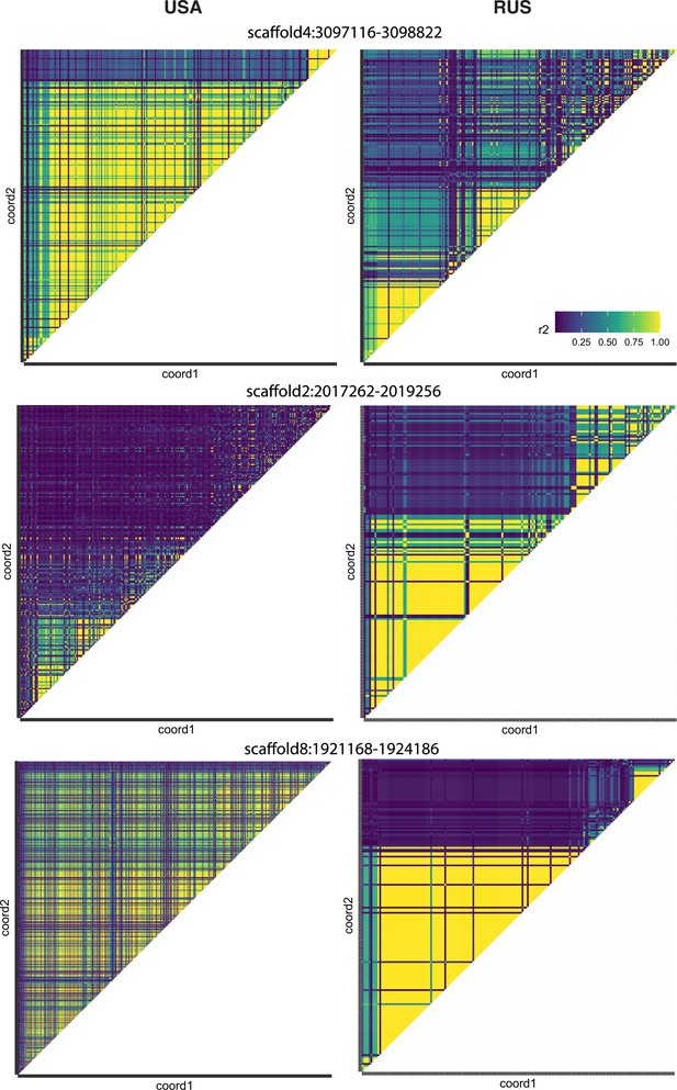
Examples of haploblocks in two populations of S. commune.
The heatmaps show LD between polymorphic SNPs in the same genomic regions in the USA and RUS populations of S. commune. Only biallelic polymorphic sites with minor allele frequency >1 are shown, the number of such sites can differ between populations.
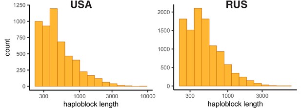
Distribution of haploblock lengths (nt) in the two populations of S. commune.
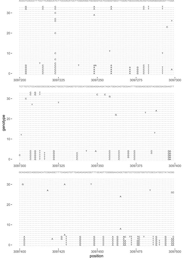
Example of the S. commune alignment within a haploblock.
Region 3097200–3097500 of scaffold 4 in the USA population of S. commune is shown. The top line shows the consensus sequence based on 34 genotypes; dot indicates match with the consensus.
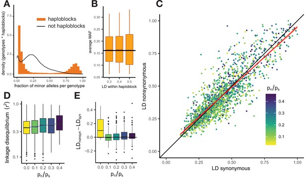
Patterns of linkage disequilibrium in the RUS population of S. commune.
(A) Bimodal distribution of the fraction of polymorphic sites carrying minor alleles per genome within the haploblocks. Each count corresponds to a genotype within a haploblock. Black line shows the background distribution of minor alleles in the non-haploblock regions. (B) The increased average minor allele frequency within haploblocks as compared to the non-haploblock regions (dashed line, t-test p-value <2e-16). (C) LD between nonsynonymous and synonymous SNPs within single genes. Each dot represents an individual gene. Linear regression of LDnonsyn over LDnsyn is shown as the red line. To control for the gene length, only SNPs within 300 bp from each other were analyzed. Genes with fewer than 100 such pairs of SNPs were excluded. (D,E) The positive correlation between pn/ps of the gene and its average LD (Spearman correlation p-value = 4e-16) (D) or the difference between LDnonsyn and LDsyn (Spearman correlation p-value = 2e-5) (E).
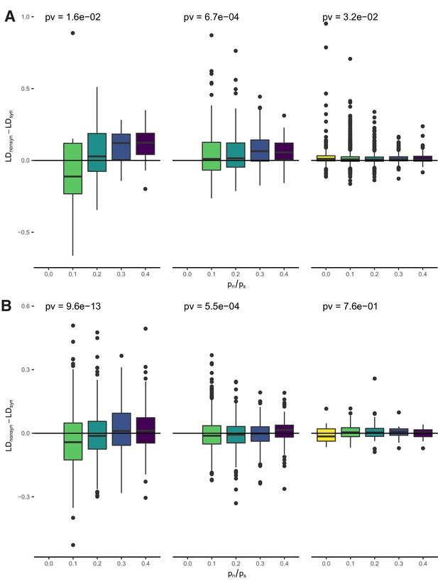
Comparison of LDnonsyn and LDsyn in the genes of S. commune.
(A) The USA population, (B) the RUS population. The genes are stratified by their average LD (the panels) and by the pn/ps. Only pairs of SNPs within 300 bp from each other are analyzed; genes with less than 100 such pairs of nonsynonymous or synonymous SNPs are excluded. Spearman correlation p-values are shown.
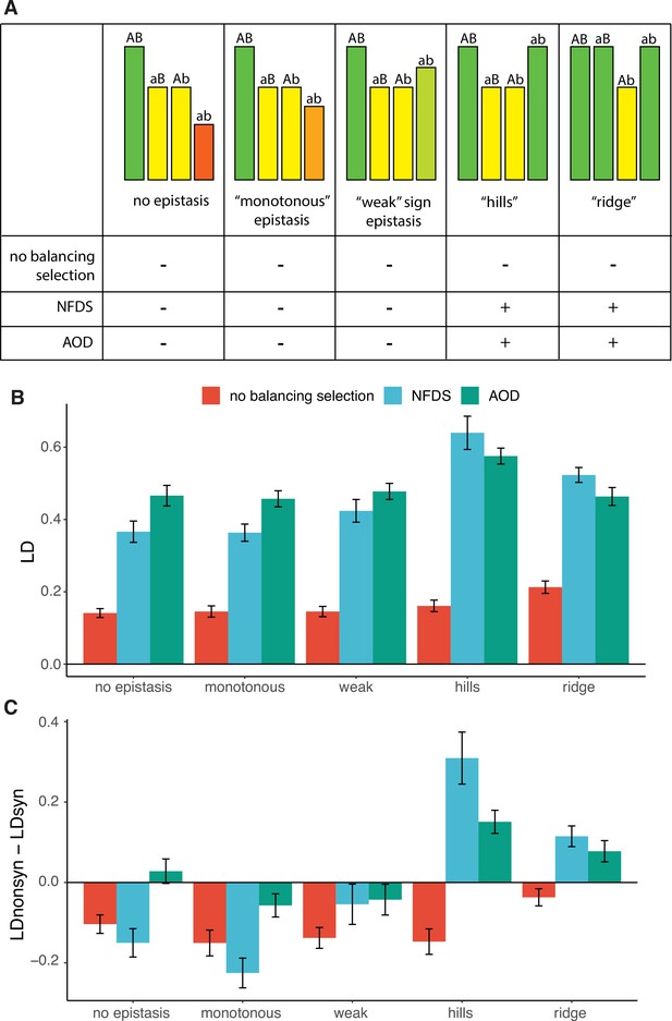
The difference between LDnonsyn and LDsyn under pairwise epistasis and balancing selection.
(A) The excess of LDnonsyn over LDsyn under different models of epistasis between two deleterious mutations A → a and B → b without balancing selection and in the presence of negative frequency-dependent selection (NFDS) or associate overdominance (AOD) acting in the linked sites. The height of columns shows fitness of the corresponding genotypes. (+) indicate simulations where the excess of LDnonsyn is reproduced. (B) The average LD in the simulations. (C) The difference between LDnonsyn and LDsyn in the simulations.

Criteria for haploblocks in S. commune.
Red lines show the distribution of LD (r2) in windows of 250 nucleotides in two populations. Black line corresponds to the lognormal distribution with the same mean and variance. The windows with LD higher than the threshold value defined as the intersection point of the two lines (dashed) are attributed to haploblocks.
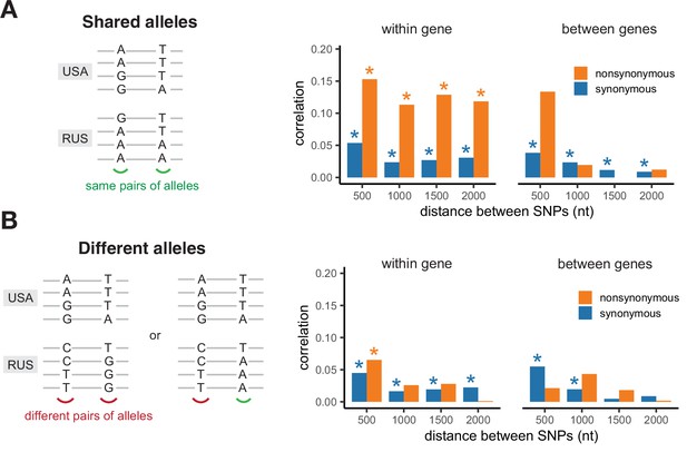
Correlation of LD values between pairs of shared SNPs in the two S. commune populations.
(A) Pairs of SNPs with the same alleles in both sites, (B) pairs of SNPs differing by at least one allele. Asterisks indicate Spearman correlation p-values <0.001.
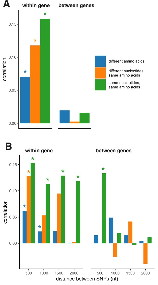
Association of LD values between pairs of shared nonsynonymous SNPs encoding the same amino acids in the two S. commune populations.
(A) All pairs of SNPs pooled together. Pair of SNPs is considered to carry different alleles if at least one allele differs in at least one site. (B) Pairs of SNPs stratified by distance between them. Asterisks indicate Spearman correlation p-values <0.01.
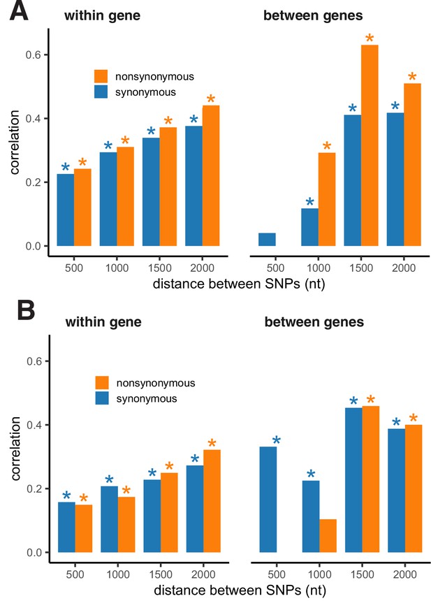
Association of LD values between pairs of shared SNPs within haploblocks in the two S. commune populations.
(A) Pairs of SNPs with the same major and minor alleles in both sites, (B) pairs of SNPs differing by at least one allele. Asterisks indicate Spearman correlation p-values <0.001.
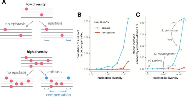
The efficiency of epistasis in populations with different levels of nucleotide diversity.
(A) Under low nucleotide diversity, deleterious mutations (red dots) are unlikely to be compensated. If nucleotide diversity is high, epistatic selection maintains LD between SNPs in interacting sites (blue dots). (B) The probability that a deleterious variant is compensated by another variant within the same individual at the end of the simulation. (C) Increase in the mean fitness of the population caused by epistatic selection maintaining LD between favorable allele combinations. The fitness is plotted relative to that of a population consisting of individuals with uncorrelated alleles at different sites, obtained by permuting alleles among individuals. The efficiency of epistatic selection in maintaining linkage is much higher in genetically variable populations. Asterisks in (C) indicate significant deviation from 0 (Wilcoxon paired test p-value <0.01). Each simulation was repeated between 100 and 10,000 times depending on genetic diversity.
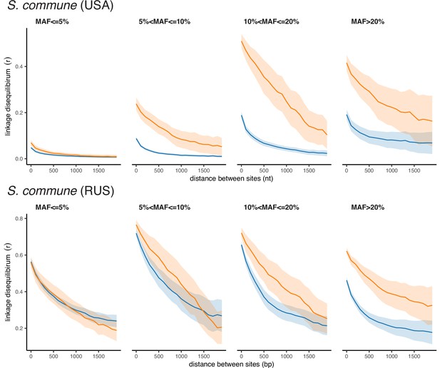
Polarized linkage disequilibrium in S. commune.
LD between nonsynonymous SNPs is shown in orange, and LD between synonymous SNPs is shown in blue. Filled areas indicate SE of LD calculated for each scaffold separately.
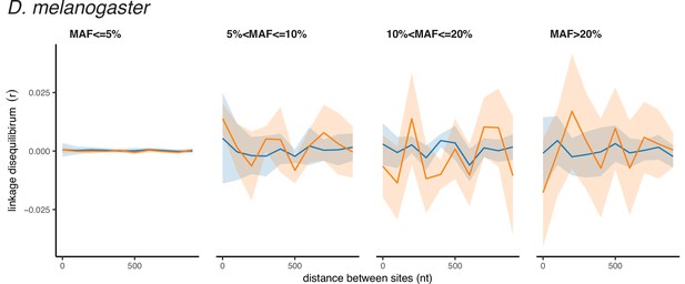
Polarized linkage disequilibrium in D. melanogaster.
LD between nonsynonymous SNPs is shown in orange, and LD between synonymous SNPs is shown in blue. Filled areas indicate SE of LD calculated for each chromosome separately.
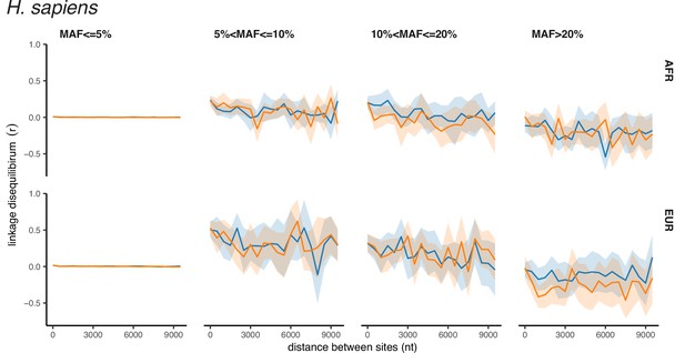
Polarized linkage disequilibrium in H. sapiens.
LD between nonsynonymous SNPs is shown in orange, and LD between synonymous SNPs is shown in blue. Filled areas indicate SE of LD calculated for each chromosome separately.
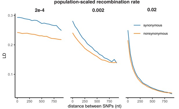
LDnonsyn and LDsyn in simulations under weak negative selection.
LD between synonymous (blue, selection coefficient Nes = 0) and nonsynonymous (orange, Nes = –1) variants under varying recombination rate. Only SNPs with MAF >0.05 are shown. Simulated haploid population size N=2000, sequence length L=1000 bp.
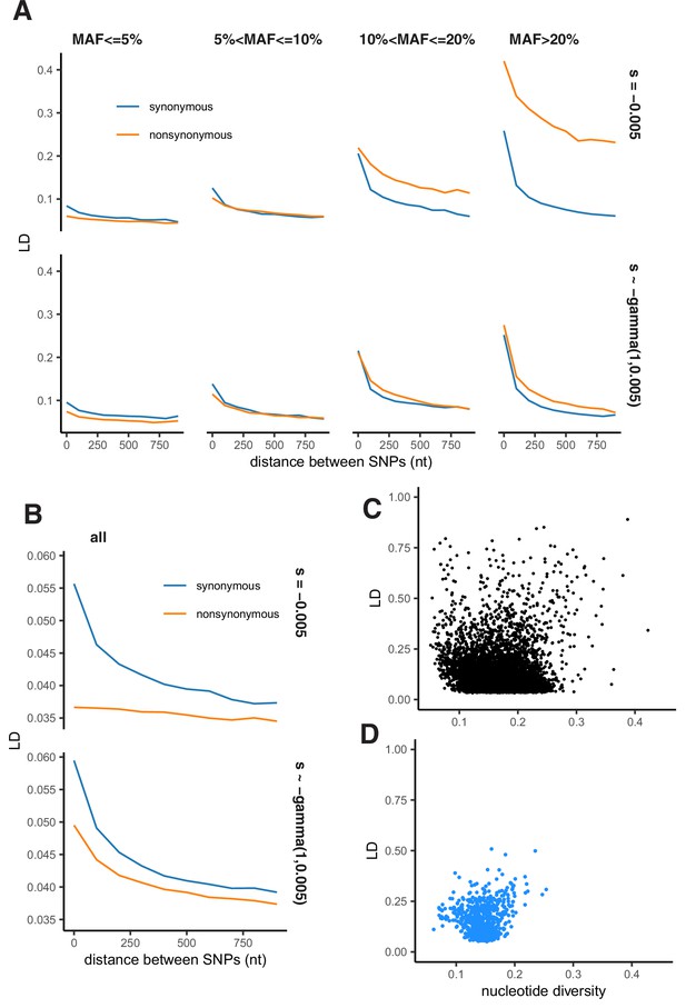
Patterns of LD in simulations under Hill-Robertson interference.
(A) LD between nonsynonymous and synonymous pairs of SNPs split by MAF. (B) LD between all pairs of nonsynonymous and synonymous SNPs pooled together. (A–B) Simulated haploid population size N=2000, sequence length L=1000 bp. Top panels - selection coefficients of all nonsynonymous mutations are equal to –0.005 (Nes = –10); bottom panels - selection coefficients of nonsynonymous mutations are gamma-distributed with parameters rate = 1, scale = 0.005. (C) LD and nucleotide diversity within genes of the USA population of S. commune (each point represents one gene). (D) LD and nucleotide diversity obtained in simulations.
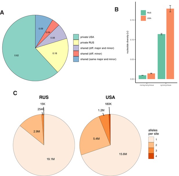
Patterns of nucleotide diversity in S. commune.
(A) The fraction of private and shared biallelic SNPs. (B) Within-population nucleotide diversity at different classes of sites (measured as π without Jukes-Cantor correction). (C) The number of monomorphic and polymorphic sites in the multiple whole-genome alignments of S. commune genomes.
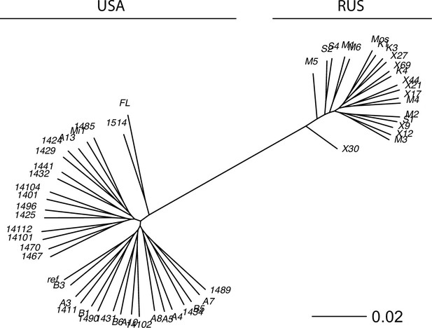
The reconstructed phylogeny of S. commune.
USA and Russian populations of S. commune are highly divergent while having almost no within-population structure. Genetic distance is measured in nucleotide differences, the phylogeny is reconstructed based on the multiple whole-genome alignment.
Tables
List of genes with pairs physically adjacent protein sites be under higher LD than pairs of distant sites.
p-values are calculated with chi-square test and adjisted using Benjamini-Hochberg multiple testing correction.
| cog number | 90% r2 quantile | # distant & high LD | # close & high LD | # distant & low LD | # close & low LD | OR | p-value | q-value | aligned PDB ID |
|---|---|---|---|---|---|---|---|---|---|
| RUS population | |||||||||
| 10,789 | 1.00 | 6 | 6 | 85 | 8 | 10.63 | 4.3E-04 | 8.4E-03 | 4N6Q A |
| 7636 | 1.00 | 40 | 16 | 263 | 11 | 9.56 | 5.2E-09 | 5.5E-07 | 4FQG A |
| 11,223 | 1.00 | 7 | 9 | 87 | 12 | 9.32 | 1.0E-04 | 2.8E-03 | 1S3S G |
| 9853 | 1.00 | 21 | 22 | 261 | 32 | 8.54 | 8.7E-11 | 1.7E-08 | 4 × 00 A |
| 17,085 | 0.19 | 16 | 6 | 183 | 11 | 6.24 | 1.6E-03 | 2.1E-02 | 1NLT A |
| 12,357 | 1.00 | 56 | 30 | 245 | 24 | 5.47 | 1.5E-08 | 1.4E-06 | 2GUY A |
| 1037 | 0.63 | 26 | 13 | 113 | 11 | 5.14 | 4.6E-04 | 8.8E-03 | 1K8F A |
| 6153 | 0.81 | 39 | 14 | 126 | 9 | 5.03 | 5.2E-04 | 9.7E-03 | 5GVH A |
| 14,273 | 0.38 | 22 | 9 | 244 | 21 | 4.75 | 7.5E-04 | 1.3E-02 | 3LCC A |
| 5725 | 0.38 | 26 | 15 | 312 | 38 | 4.74 | 1.6E-05 | 6.3E-04 | 1TA3 B |
| 18,561 | 1.00 | 69 | 32 | 558 | 55 | 4.71 | 3.0E-10 | 4.8E-08 | 1KSG A |
| 3052 | 1.00 | 91 | 25 | 222 | 13 | 4.69 | 1.3E-05 | 5.4E-04 | 4U9V B |
| 3876 | 0.80 | 38 | 22 | 373 | 47 | 4.59 | 4.1E-07 | 3.0E-05 | 1W63 A |
| 4779 | 0.68 | 80 | 26 | 873 | 63 | 4.50 | 1.6E-09 | 2.1E-07 | 2GJL A |
| 16,912 | 1.00 | 172 | 54 | 1383 | 99 | 4.39 | 9.1E-17 | 8.8E-14 | 1WKR A |
| 14,670 | 0.82 | 25 | 8 | 273 | 20 | 4.37 | 2.2E-03 | 2.6E-02 | 6C6N A |
| 14,338 | 1.00 | 110 | 28 | 150 | 9 | 4.24 | 2.8E-04 | 6.6E-03 | 6J3E A |
| 8942 | 1.00 | 35 | 10 | 279 | 19 | 4.20 | 1.1E-03 | 1.6E-02 | 3DH1 A |
| 3214 | 1.00 | 37 | 9 | 189 | 11 | 4.18 | 4.4E-03 | 4.2E-02 | 1SZN A |
| 1413 | 1.00 | 78 | 24 | 253 | 19 | 4.10 | 1.8E-05 | 6.8E-04 | 5L3Q B |
| 7650 | 1.00 | 75 | 29 | 201 | 19 | 4.09 | 1.2E-05 | 5.1E-04 | 5EBE B |
| 1071 | 1.00 | 178 | 54 | 1002 | 75 | 4.05 | 1.0E-13 | 2.4E-11 | 1SXJ D |
| 18,096 | 0.64 | 42 | 16 | 462 | 45 | 3.91 | 3.7E-05 | 1.2E-03 | 1WPX A |
| 13,142 | 0.81 | 57 | 9 | 562 | 23 | 3.86 | 1.6E-03 | 2.1E-02 | 5GHE A |
| 16,593 | 0.59 | 118 | 34 | 954 | 72 | 3.82 | 1.7E-09 | 2.1E-07 | 3WDO A |
| 14,325 | 1.00 | 133 | 28 | 621 | 36 | 3.63 | 1.1E-06 | 6.8E-05 | 5U03 A |
| 10,827 | 0.80 | 25 | 11 | 286 | 35 | 3.60 | 2.1E-03 | 2.5E-02 | 2IHO A |
| 10,077 | 0.44 | 38 | 11 | 397 | 32 | 3.59 | 1.3E-03 | 2.0E-02 | 3AKF A |
| 9626 | 0.78 | 47 | 9 | 468 | 25 | 3.58 | 3.2E-03 | 3.4E-02 | 2CVF A |
| 10,648 | 0.75 | 59 | 20 | 587 | 56 | 3.55 | 1.4E-05 | 5.6E-04 | 3I83 A |
| 8,095 | 1.00 | 192 | 60 | 1686 | 151 | 3.49 | 3.2E-14 | 1.0E-11 | 2YMU A |
| 5372 | 0.56 | 88 | 33 | 914 | 99 | 3.46 | 3.3E-08 | 2.9E-06 | 1RGI G |
| 14,269 | 1.00 | 105 | 23 | 426 | 27 | 3.46 | 4.1E-05 | 1.3E-03 | 5UJ8 E |
| 14,404 | 1.00 | 54 | 16 | 374 | 33 | 3.36 | 4.0E-04 | 8.0E-03 | 4IDA A |
| 17,420 | 0.34 | 32 | 12 | 340 | 39 | 3.27 | 2.4E-03 | 2.8E-02 | 1W9P A |
| 6507 | 0.71 | 63 | 13 | 620 | 40 | 3.20 | 9.9E-04 | 1.6E-02 | 1AUA A |
| 9423 | 1.00 | 60 | 11 | 401 | 23 | 3.20 | 4.4E-03 | 4.2E-02 | 4Y42 A |
| 7878 | 0.78 | 41 | 17 | 446 | 58 | 3.19 | 3.5E-04 | 8.0E-03 | 4TYW A |
| 3307 | 1.00 | 87 | 17 | 720 | 45 | 3.13 | 2.3E-04 | 5.8E-03 | 6DVH A |
| 6285 | 0.27 | 55 | 13 | 565 | 43 | 3.11 | 1.4E-03 | 2.1E-02 | 2VWS A |
| 10,049 | 0.83 | 68 | 16 | 668 | 51 | 3.08 | 4.0E-04 | 8.0E-03 | 1KH4 A |
| 6148 | 1.00 | 628 | 131 | 1361 | 93 | 3.05 | 1.6E-15 | 7.7E-13 | 4CHT A |
| 14,511 | 0.63 | 42 | 13 | 414 | 44 | 2.91 | 3.7E-03 | 3.7E-02 | 3HG7 A |
| 2522 | 0.23 | 46 | 16 | 492 | 60 | 2.85 | 1.5E-03 | 2.1E-02 | 5L0R A |
| 5,375 | 0.67 | 45 | 18 | 448 | 63 | 2.84 | 9.6E-04 | 1.5E-02 | 2WZO A |
| 73 | 0.21 | 68 | 20 | 715 | 74 | 2.84 | 2.5E-04 | 6.2E-03 | 1WPX A |
| 12,131 | 1.00 | 210 | 35 | 816 | 48 | 2.83 | 8.7E-06 | 4.0E-04 | 6GKV A |
| 1097 | 1.00 | 63 | 17 | 534 | 51 | 2.83 | 1.1E-03 | 1.6E-02 | 2IW0 A |
| 18,360 | 1.00 | 174 | 35 | 924 | 66 | 2.82 | 3.6E-06 | 2.0E-04 | 1ULT A |
| 5930 | 0.38 | 57 | 16 | 594 | 60 | 2.78 | 1.5E-03 | 2.1E-02 | 2 PXX A |
| 8261 | 0.81 | 112 | 42 | 930 | 129 | 2.70 | 9.4E-07 | 6.5E-05 | 4QNW A |
| 18,092 | 1.00 | 83 | 22 | 794 | 78 | 2.70 | 2.5E-04 | 6.1E-03 | 4QJY A |
| 1060 | 0.78 | 65 | 16 | 533 | 50 | 2.62 | 3.2E-03 | 3.3E-02 | 3WXB A |
| 17,037 | 0.31 | 95 | 19 | 918 | 70 | 2.62 | 7.4E-04 | 1.3E-02 | 5YHP A |
| 15,353 | 1.00 | 109 | 26 | 944 | 86 | 2.62 | 1.0E-04 | 2.8E-03 | 3WNV A |
| 7784 | 1.00 | 120 | 15 | 929 | 45 | 2.58 | 3.5E-03 | 3.5E-02 | 3L4G B |
| 10,236 | 0.53 | 182 | 35 | 1810 | 135 | 2.58 | 3.5E-06 | 2.0E-04 | 1Q6X A |
| 2011 | 0.34 | 90 | 17 | 889 | 67 | 2.51 | 2.4E-03 | 2.7E-02 | 3A1K A |
| 8572 | 1.00 | 167 | 32 | 976 | 76 | 2.46 | 8.1E-05 | 2.4E-03 | 4AH6 A |
| 14,282 | 0.81 | 153 | 18 | 1251 | 60 | 2.45 | 2.0E-03 | 2.4E-02 | 3QM4 A |
| 7836 | 0.78 | 83 | 17 | 685 | 58 | 2.42 | 4.4E-03 | 4.2E-02 | 1DQW A |
| 3610 | 0.46 | 196 | 45 | 1946 | 185 | 2.42 | 1.2E-06 | 7.3E-05 | 4BKX B |
| 8725 | 0.63 | 71 | 18 | 669 | 71 | 2.39 | 4.0E-03 | 4.0E-02 | 6G6M A |
| 11,096 | 0.48 | 64 | 20 | 657 | 87 | 2.36 | 3.0E-03 | 3.2E-02 | 3AKF A |
| 6520 | 0.75 | 86 | 28 | 599 | 84 | 2.32 | 8.3E-04 | 1.4E-02 | 4K3A A |
| 12,399 | 1.00 | 610 | 107 | 994 | 76 | 2.29 | 1.4E-07 | 1.1E-05 | 1JZQ A |
| 8945 | 1.00 | 147 | 32 | 558 | 53 | 2.29 | 7.9E-04 | 1.3E-02 | 3E5M A |
| 1744 | 1.00 | 148 | 45 | 616 | 83 | 2.26 | 9.7E-05 | 2.8E-03 | 1C7J A |
| 16,360 | 0.82 | 134 | 34 | 1297 | 149 | 2.21 | 2.0E-04 | 5.3E-03 | 3WTC A |
| 12,853 | 0.53 | 168 | 31 | 1634 | 139 | 2.17 | 3.8E-04 | 8.0E-03 | 6H7D A |
| 14,137 | 0.64 | 118 | 27 | 1175 | 127 | 2.12 | 1.7E-03 | 2.1E-02 | 6C5B A |
| 7106 | 0.38 | 124 | 22 | 1167 | 98 | 2.11 | 4.4E-03 | 4.2E-02 | 5K8E A |
| 1523 | 1.00 | 77 | 29 | 402 | 72 | 2.10 | 4.4E-03 | 4.2E-02 | 5Y1B A |
| 2779 | 0.68 | 127 | 27 | 1155 | 120 | 2.05 | 2.8E-03 | 3.0E-02 | 1SXJ B |
| 4275 | 1.00 | 555 | 87 | 957 | 74 | 2.03 | 2.5E-05 | 8.4E-04 | 5VC7 A |
| 17,782 | 1.00 | 184 | 53 | 581 | 83 | 2.02 | 4.1E-04 | 8.0E-03 | 4QNW A |
| 4829 | 1.00 | 350 | 62 | 504 | 46 | 1.94 | 1.7E-03 | 2.1E-02 | 5MXC A |
| 9827 | 0.46 | 237 | 42 | 2273 | 209 | 1.93 | 3.9E-04 | 8.0E-03 | 2VJY A |
| 1520 | 0.45 | 153 | 32 | 1498 | 163 | 1.92 | 2.6E-03 | 2.9E-02 | 3PQV A |
| 4468 | 1.00 | 238 | 48 | 1409 | 148 | 1.92 | 3.6E-04 | 8.0E-03 | 1V9L A |
| 8360 | 1.00 | 852 | 74 | 884 | 40 | 1.92 | 1.5E-03 | 2.1E-02 | 5YLW A |
| 16,987 | 0.53 | 154 | 34 | 1482 | 174 | 1.88 | 2.8E-03 | 3.0E-02 | 3LWT X |
| 935 | 0.65 | 104 | 38 | 1036 | 203 | 1.86 | 3.0E-03 | 3.2E-02 | 3FGA A |
| 11,732 | 0.68 | 118 | 40 | 1076 | 196 | 1.86 | 2.3E-03 | 2.7E-02 | 4C2L A |
| 15,295 | 0.82 | 152 | 41 | 1326 | 193 | 1.85 | 1.7E-03 | 2.1E-02 | 4A69 A |
| 6753 | 1.00 | 246 | 36 | 1868 | 151 | 1.81 | 3.4E-03 | 3.5E-02 | 1SXJ C |
| 13,863 | 1.00 | 319 | 86 | 414 | 62 | 1.80 | 1.6E-03 | 2.1E-02 | 6F43 A |
| USA population | |||||||||
| 14,970 | 0.53 | 13 | 6 | 160 | 8 | 9.23 | 1.8E-04 | 1.3E-02 | 2VFR A |
| 1536 | 0.65 | 12 | 13 | 184 | 23 | 8.67 | 4.6E-07 | 2.0E-04 | 6AHR E |
| 3618 | 0.20 | 9 | 10 | 139 | 24 | 6.44 | 2.1E-04 | 1.4E-02 | 5LCL B |
| 18,366 | 0.11 | 44 | 15 | 486 | 41 | 4.04 | 3.5E-05 | 4.5E-03 | 1UPU D |
| 8253 | 0.16 | 44 | 12 | 467 | 35 | 3.64 | 5.8E-04 | 3.4E-02 | 6F87 A |
| 9241 | 0.16 | 56 | 23 | 624 | 81 | 3.16 | 2.6E-05 | 4.2E-03 | 1YCD A |
| 1743 | 0.15 | 49 | 19 | 510 | 64 | 3.09 | 2.1E-04 | 1.4E-02 | 4PEH A |
| 64 | 0.15 | 85 | 27 | 905 | 101 | 2.85 | 1.9E-05 | 3.6E-03 | 2B4Q A |
| 14,128 | 0.11 | 77 | 28 | 804 | 103 | 2.84 | 1.9E-05 | 3.6E-03 | 2 × 8 R A |
| 10,841 | 0.16 | 120 | 20 | 1166 | 69 | 2.82 | 1.5E-04 | 1.2E-02 | 3TIK A |
| 17,174 | 0.64 | 96 | 27 | 679 | 73 | 2.62 | 1.4E-04 | 1.2E-02 | 5EY6 A |
| 5725 | 0.11 | 73 | 30 | 799 | 126 | 2.61 | 5.9E-05 | 6.9E-03 | 1TA3 B |
| 10,834 | 0.37 | 90 | 31 | 936 | 124 | 2.60 | 3.3E-05 | 4.5E-03 | 2QB6 A |
| 1267 | 0.24 | 117 | 29 | 1150 | 116 | 2.46 | 1.0E-04 | 1.0E-02 | 4CPD A |
| 9614 | 0.16 | 149 | 44 | 1550 | 187 | 2.45 | 1.9E-06 | 6.0E-04 | 2VGL B |
| 6148 | 0.53 | 487 | 75 | 4438 | 284 | 2.41 | 1.2E-10 | 1.5E-07 | 4CHT A |
| 161 | 0.10 | 227 | 52 | 2,206 | 210 | 2.41 | 2.0E-07 | 1.3E-04 | 5DNC A |
| 621 | 0.10 | 105 | 35 | 1060 | 152 | 2.32 | 9.1E-05 | 9.7E-03 | 3WG6 A |
| 14,368 | 0.09 | 124 | 26 | 1008 | 92 | 2.30 | 7.4E-04 | 4.1E-02 | 2 × 1 C A |
| 9215 | 0.31 | 161 | 56 | 1546 | 243 | 2.21 | 3.0E-06 | 7.6E-04 | 4QNW A |
| 13,117 | 0.47 | 140 | 44 | 1401 | 226 | 1.95 | 4.5E-04 | 2.8E-02 | 1W9P A |
| 3876 | 0.28 | 232 | 51 | 2244 | 259 | 1.90 | 1.5E-04 | 1.2E-02 | 1W63 A |
Assembly statistics of 24 genomes of S. commune (14 samples from USA population and 7 samples from RUS population).
| sample id | specimen voucher | origin | # contigs | total length (bp) | largest contig (bp) | GC % | N50 | coverage |
|---|---|---|---|---|---|---|---|---|
| 14–01_S62 | WS-M161 | USA; Ann Arbor | 2462 | 37,201,238 | 674,015 | 57.5 | 153,743 | 113.2 |
| 14–101_S73 | WS-M180 | USA; Ann Arbor | 2161 | 36,629,295 | 950,471 | 57.6 | 208,079 | 74.2 |
| 14–102_S74 | WS-M181 | USA; Ann Arbor | 2895 | 37,669,799 | 959,240 | 57.6 | 146,599 | 67.8 |
| 14–104_S75 | WS-M183 | USA; Ann Arbor | 2750 | 37,829,033 | 655,066 | 57.6 | 151,136 | 75.8 |
| 14–112_S77 | WS-M191 | USA; Ann Arbor | 2577 | 37,171,981 | 838,910 | 57.6 | 173,824 | 124.5 |
| 14–11_S63 | WS-M188 | USA; Ann Arbor | 2634 | 37,679,657 | 658,404 | 57.6 | 158,664 | 64.0 |
| 14–25_S64 | WS-M206 | USA; Ann Arbor | 2762 | 38,042,099 | 976,161 | 57.6 | 160,044 | 93.8 |
| 14–29_S65 | WS-M210 | USA; Ann Arbor | 2665 | 37,691,449 | 675,061 | 57.5 | 158,777 | 95.9 |
| 14–31_S66 | WS-M212 | USA; Ann Arbor | 2453 | 37,348,833 | 870,814 | 57.5 | 161,384 | 100.0 |
| 14–32_S67 | WS-M213 | USA; Ann Arbor | 2923 | 37,685,895 | 696,590 | 57.6 | 145,350 | 62.9 |
| 14–34_S68 | WS-M215 | USA; Ann Arbor | 2455 | 37,403,482 | 951,844 | 57.5 | 185,879 | 89.2 |
| 14–67_S84 | WS-M247 | USA; Ann Arbor | 2900 | 37,778,589 | 850,026 | 57.6 | 195,995 | 70.8 |
| 14–70_S69 | WS-M247 | USA; Ann Arbor | 2809 | 37,546,616 | 678,024 | 57.6 | 154,362 | 91.4 |
| 14–85_S70 | WS-M265 | USA; Ann Arbor | 2347 | 37,174,196 | 875,526 | 57.6 | 176,501 | 45.3 |
| 14–89_S71 | WS-M269 | USA; Ann Arbor | 2352 | 37,218,933 | 959,111 | 57.6 | 177,695 | 111.6 |
| 14–90_S72 | WS-M270 | USA; Ann Arbor | 2957 | 37,322,559 | 739,843 | 57.6 | 139,455 | 110.3 |
| 15–14_S76 | WS-M292 | USA; Florida | 2460 | 37,328,560 | 616,845 | 57.6 | 157,189 | 71.5 |
| X-12_S79 | WS-M12 | Russia; Moscow | 3879 | 38,221,043 | 496,668 | 57.6 | 75,624 | 117.4 |
| X-17_S80 | WS-M18 | Russia; Moscow | 3738 | 37,604,751 | 396,219 | 57.6 | 71,000 | 105.9 |
| X-21_S81 | WS-M22 | Russia; Moscow | 5012 | 39,204,396 | 341,967 | 57.6 | 63,280 | 77.3 |
| X-27_S82 | WS-M28 | Russia; Moscow | 3571 | 37,399,774 | 525,346 | 57.6 | 71,903 | 78.2 |
| X-30_S83 | WS-M31 | Russia; Moscow | 4487 | 38,310,778 | 384,708 | 57.6 | 66,442 | 84.7 |
| X-69_S85 | WS-M70 | Russia; Moscow | 3965 | 38,348,248 | 485,689 | 57.6 | 70,802 | 76.7 |
| X-9_S78 | WS-M9 | Russia; Moscow | 4590 | 38,741,959 | 540,017 | 57.6 | 67,770 | 74.8 |


