Landscape of epithelial–mesenchymal plasticity as an emergent property of coordinated teams in regulatory networks
- Centre for BioSystems Science and Engineering, Indian Institute of Science Bangalore, India
- Department of Biotechnology, RV College of Engineering, India
- Department of Biotechnology, PES University, India
Figures
Figure 1 with 2 supplements
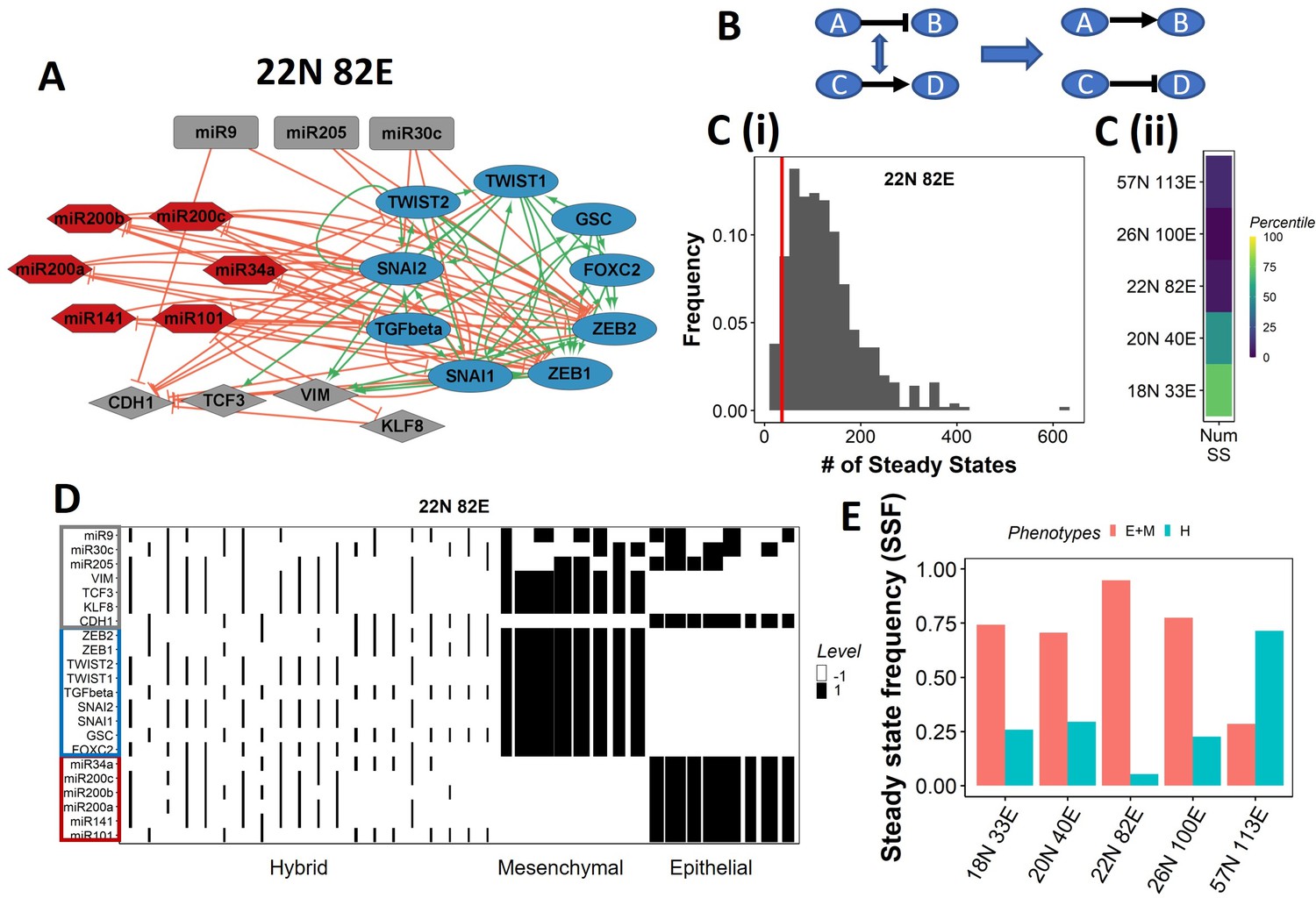
Epithelial–mesenchymal plasticity (EMP) network topology can result in a bimodal phenotypic stability landscape.
(A) EMP network of size 22N 82E, where N stands for number of nodes and E stands for number of edges. (B) Demonstration of network randomization. (C) (i) Distribution of number of steady states in random networks of size 22N 82E. The wild-type EMP network of the same size is represented using the red line. (ii) Percentile of the WT network in the distribution of the number of steady states in random networks. (D) Heatmap depicting the steady states of the 22N 82E network. Each column represents a steady state. Each row represents a node. White cells indicate low-expressing/inactive node (–1) in a state and black cells indicate high expression/active (1). The width of each column is proportional to the frequency of the given steady state. (E) Comparison of the cumulative frequency of the terminal (epithelial and mesenchymal) states vs. that of the hybrid states for all five EMP networks.
Figure 1—figure supplement 1

EMP networks and their steady state pattems.
(A) Epithelial–mesenchymal plasticity (EMP) networks of size (i) 18N 33E, (ii) 20N 40E, (iii) 26N 100E, and (iv) 57N 113E, where N stands for number of nodes and E stands for number of edges. (B) Table for the number of observed steady states and the number of possible states for wild-type (WT) EMP networks.
Figure 1—figure supplement 2
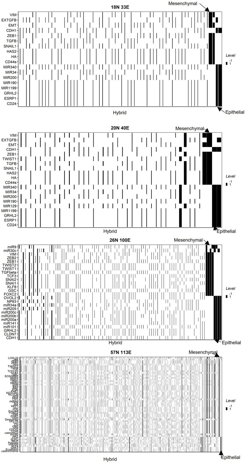
Heatmaps depicting the steady states of the epithelial–mesenchymal plasticity (EMP) networks.
Each row represents the activity of a node (–1 or 1), and each column represents a steady state.
Figure 2 with 1 supplement
Dynamic traits of phenotypes observed from wild-type (WT) epithelial–mesenchymal plasticity (EMP) networks and their randomized counterparts.
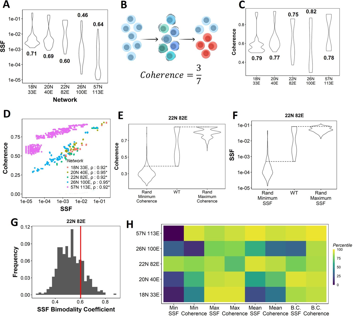
(A) Distribution of steady-state frequency (SSF) of the steady states obtained for the five EMP networks, in log10 scale. The corresponding Sarle’s bimodality coefficients have been reported. A value greater than 0.55 indicates bimodality. (B) Depiction of coherence calculation. The blue balls indicate unperturbed steady state (P1, say). The green and dark blue balls represent the perturbations given to the steady state. The red balls represent a different steady state that the system reached after the perturbation. The fraction of perturbations that reverted to the original state P1 (3 out of 7 balls) is calculated as coherence. (C) Similar to (A), but for coherence of the steady states of WT EMP networks. (D) Scatterplot between coherence and SSF of WT EMP networks. Spearman’s correlation coefficient for each network has been reported. *p<0.05. (E) Comparison of the distribution of coherence of the steady states of WT EMP network (22N 82E), with the distribution of maximum coherence values and minimum coherence values of the corresponding random networks. (F) Similar to (E), but for SSF. (G) Distribution of the SSF bimodality coefficients for random networks of size 22N 82E. The red vertical line represents the WT network. (H) Percentile of the WT networks in the distribution of multiple stability metrics obtained from random networks.
Figure 2—figure supplement 1

Coherence and steady-state frequencies for EMP networks.
(A) Comparison of the distribution of coherence of the steady states of wild-type (WT) epithelial–mesenchymal plasticity (EMP) networks with the distribution of maximum SSF values and minimum SSF values of the corresponding random networks. (B) Same as (A) but for steady state frequency (SSF). (C) Distribution of the SSF bimodality coefficients for random networks corresponding to WT EMP networks. The corresponding WT network in each panel is represented by the red vertical line. (D) Same as (C) but for coherence.
Figure 3 with 1 supplement
Frustration as a stability metric for wild-type (WT) and random networks.
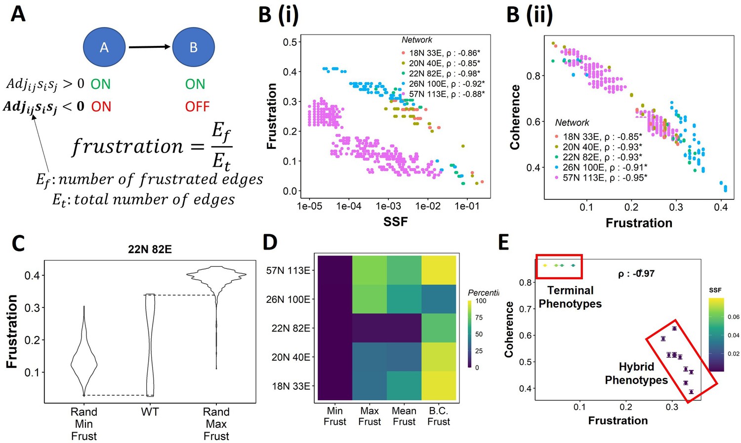
(A) Depiction of calculation of frustration. represents the interaction from ith node to jth node, si and sj represent the activity of the ith node and the jth node for a given state . (B) Scatterplot between frustration and (i) steady-state frequency (SSF), (ii) coherence for WT epithelial–mesenchymal plasticity (EMP) networks. Spearman’s correlation coefficient for each network has been reported. *p<0.05. Each dot corresponds to a steady state for the given network. (C) Comparison of the distribution of frustration of the steady states of WT EMP network (22N 82E), with the distribution of maximum frustration values and minimum frustration values of the corresponding random networks. (D) Heatmap of the percentile of WT network values in the random network value distribution for the minimum, maximum, and mean frustration. (E) Representation of WT steady states in a scatterplot of frustration and coherence with the color representing the corresponding SSF. Spearman’s correlation coefficient between the axis metrics is reported. *p<0.05. The terminal and hybrid phenotypes are highlighted with red rectangles.
Figure 3—figure supplement 1
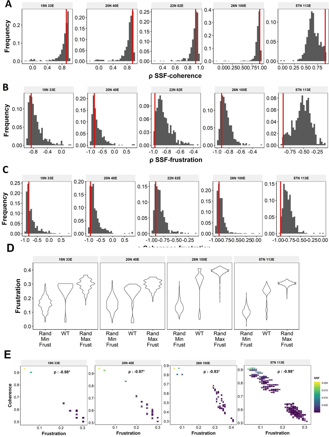
Association among SSF, coherence and frustration across EMP networks.
(A–C) Distribution of Spearman’s correlation coefficient of (A) steady-state frequency (SSF) – coherence, (B) SSF – frustration, and (C) coherence – frustration for random networks corresponding to wild-type (WT) epithelial–mesenchymal plasticity (EMP) networks. The corresponding WT network in each panel is represented by the red vertical line. (D) Comparison of the distribution of frustration of the steady states of WT EMP networks with the distribution of maximum frustration values and minimum frustration values of the corresponding random networks. (E) Representation of WT steady states in a 2D stability axes with color as SSF.
Figure 4 with 2 supplements
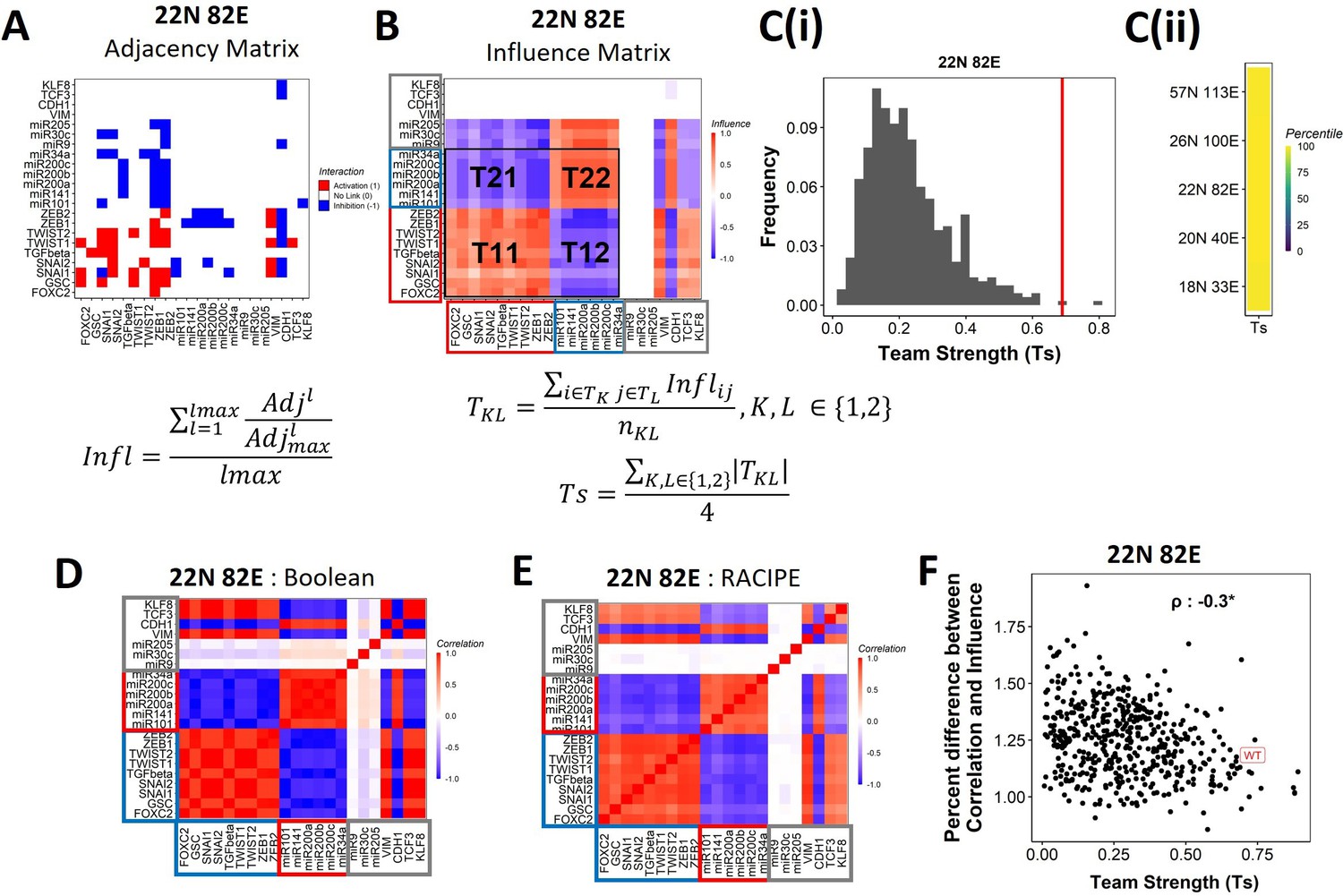
Epithelial–mesenchymal plasticity (EMP) networks consist of two well-coordinated teams.
(A) Adjacency matrix of the 22N 82E network. Each row depicts the links originating from the node (i.e., input) corresponding to the row (y-axis) and all other nodes (x-axis, outputs). The color represents the nature of the edge: red for activating links, blue for inhibiting links, and white for no links. The formula for the conversion of adjacency matrix to influence matrix is given below the panel, where is the adjacency matrix, is the adjacency matrix with all –1s replaced with 1s. is the adjacency matrix raised to the power of . The division is element-wise. is the maximum path length considered for calculating the influence. (B) The influence matrix for the 22N 82E network. The signal and output nodes (peripheral) are highlighted with a gray box, the mesenchymal nodes (team 1) are highlighted with a blue box, and the epithelial nodes (team 2) are highlighted with a red box. The formula for team strength (Ts) is given below the influence matrix. T1 and T2 represent the two teams of nodes in the network (epithelial and mesenchymal nodes, respectively). is the number of cells in the rectangle (C) (i) Distribution of team strength (Ts) for random networks of size 22N 82E. The Ts value for the corresponding wild-type (WT) EMP network has been highlighted using the red vertical line. (ii) Percentiles corresponding to the WT team strength in the corresponding distribution obtained from random networks for networks of all sizes (y-axis). (D) Correlation matrix for the expression levels of nodes of the 22N 82E network, as obtained by the Boolean formalism. (E) Same as (D) but for RAndom CIrcuit PErturbaiton (RACIPE). (F) Scatterplot of the difference between the influence matrix and Boolean correlation matrix (y-axis) and the mean group strength of the network (x-axis) for random networks of size 22N 82E. The wild-type EMP network is highlighted in red. Spearman’s correlation coefficient is reported. *p<0.05.
Figure 4—figure supplement 1

Influence matrices and correlation matrices for EMP networks.
(A) Influence matrices for the epithelial–mesenchymal plasticity (EMP) networks. (B) Distribution of the team strength (Ts) for EMP networks (i) 18N 33E, (ii) 20N 40E, and (ii) 26N 100E. (C) Correlation matrices for Boolean expression levels of EMP networks, in increasing order of number of nodes except for 22N 82E network. (D) Same as (C) but for RAndom CIrcuit PErturbaiton (RACIPE). (E) Similar to Figure 2F, for networks other than 22N 82E.
Figure 4—figure supplement 2
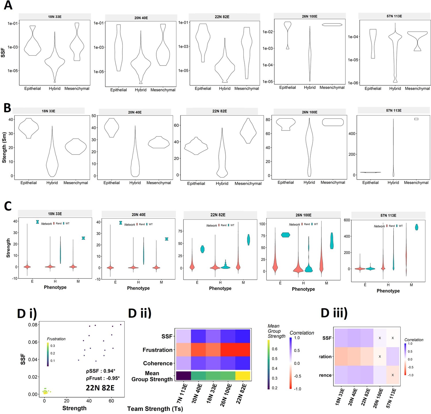
Steady-state frequency and state strength calculations for EMP networks.
(A) Distribution ofsteady-state frequency(SSF)for theRAndom CIrcuit PErturbaiton(RACIPE)states of22N82Ewild-type (WT)epithelial–mesenchymal plasticity(EMP)network.The state classification is done based on teams identified in (B). (B) Distribution of the strength of states of the EMP networks from RACIPE. (C) Comparisonof the state strength distributions forepithelial,mesenchymal,andhybrid phenotypes obtained from WT and random networks of labelled sizes. (D) (i) Correlation of state strength with SSF andfrustration for22N82E WT network. (ii) Correlation between the stability metrics (y-axis) and the strength for the states of the five different WT EMP networks (x-axis). The team strengths of the networksarerepresented using a different color scheme at the bottom of the heatmap. (iii) Correlation between the quantities in (D(ii)) and Gs for random networks of corresponding to WT networks of different sizes.
Figure 5 with 2 supplements
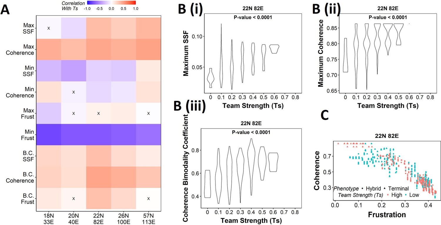
Strong teams support the bimodal epithelial–mesenchymal plasticity (EMP) landscape.
(A) Heatmap depicting the Spearman’s correlation of Ts with stability metrics and frustration metrics for random networks of all sizes (y-axis). Insignificant correlations (p>0.05) are marked by ‘X.’ (B) Violin plots depicting the effect of change in Ts against the maximum stability metrics. (i) Maximum steady-state frequency (SSF), (ii) maximum coherence, and (iii) coherence bimodality coefficient for random networks of size 22N 82E. The p-value for one-way ANOVA is reported. (C) Scatterplot showing the states of top 10 and bottom 10 (based on mean group strength) random networks of size 22N 82E.
Figure 5—figure supplement 1

Violin plots depicting the effect of change in Team Strength (Ts) against the maximum stability metrics.
(A) Maximum steady-state frequency (SSF), (B) maximum coherence, and (C) coherence bimodality coefficient for random networks of size 22N 82E. The p-value for one-way ANOVA is reported. (D) Scatterplot showing the states of top 10 and bottom 10 (based on mean group strength) random networks of corresponding sizes labeled.
Figure 5—figure supplement 2
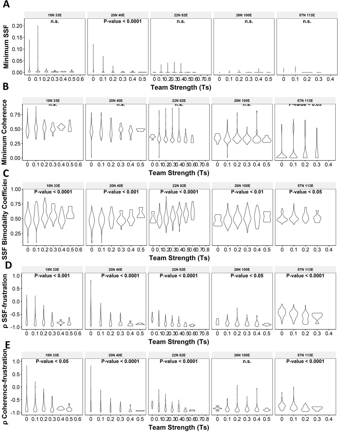
Violin plots depicting the effect of change in team strength (Ts) against the minimum stability metrics.
(A) Minimum steady-state frequency (SSF), (B) minimum coherence, and (C) SSF bimodality coefficient. (D–F) Same as (A–C) but for Spearman’s correlation between (D) SSF – frustration, (E) coherence – frustration, and (F) SSF – coherence.
Figure 6 with 2 supplements
Teams of nodes impart distinct dynamic properties to terminal and hybrid phenotypes.
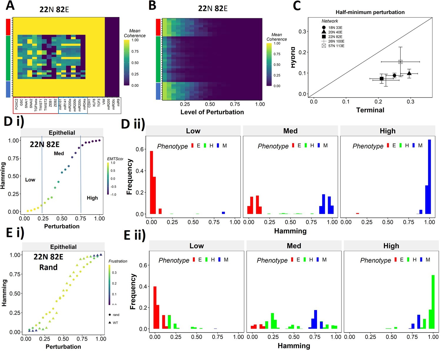
(A) Heatmap depicting the mean coherence of the Boolean states of 22N 82E wild-type (WT) epithelial–mesenchymal plasticity (EMP) network when each node is individually perturbed. (B) Mean coherence of states of 22N 82E EMP network with multiple nodes perturbed at once (Level of perturbation). (C) The extent of perturbation required to bring the coherence of terminal phenotypes (x-axis) and hybrid phenotypes (y-axis) below 0.5. x = y line is shown. (D) (i) Representative mean Hamming distance plot of an epithelial state obtained from 22N 82E WT network. Three levels of perturbation are highlighted based on regions of the sigmoidal plot. (ii) Distribution of the Hamming distance from the starting state in (D) (i) at different levels of perturbation, colored by the phenotype. (E) (i) Representative mean Hamming distance plot comparing the dynamic transition of an epithelial state from WT and that from a random network. (ii) Corresponding distribution of Hamming distances for the random network.
Figure 6—figure supplement 1
Single and multinode perturbation of WT and random EMP networks.
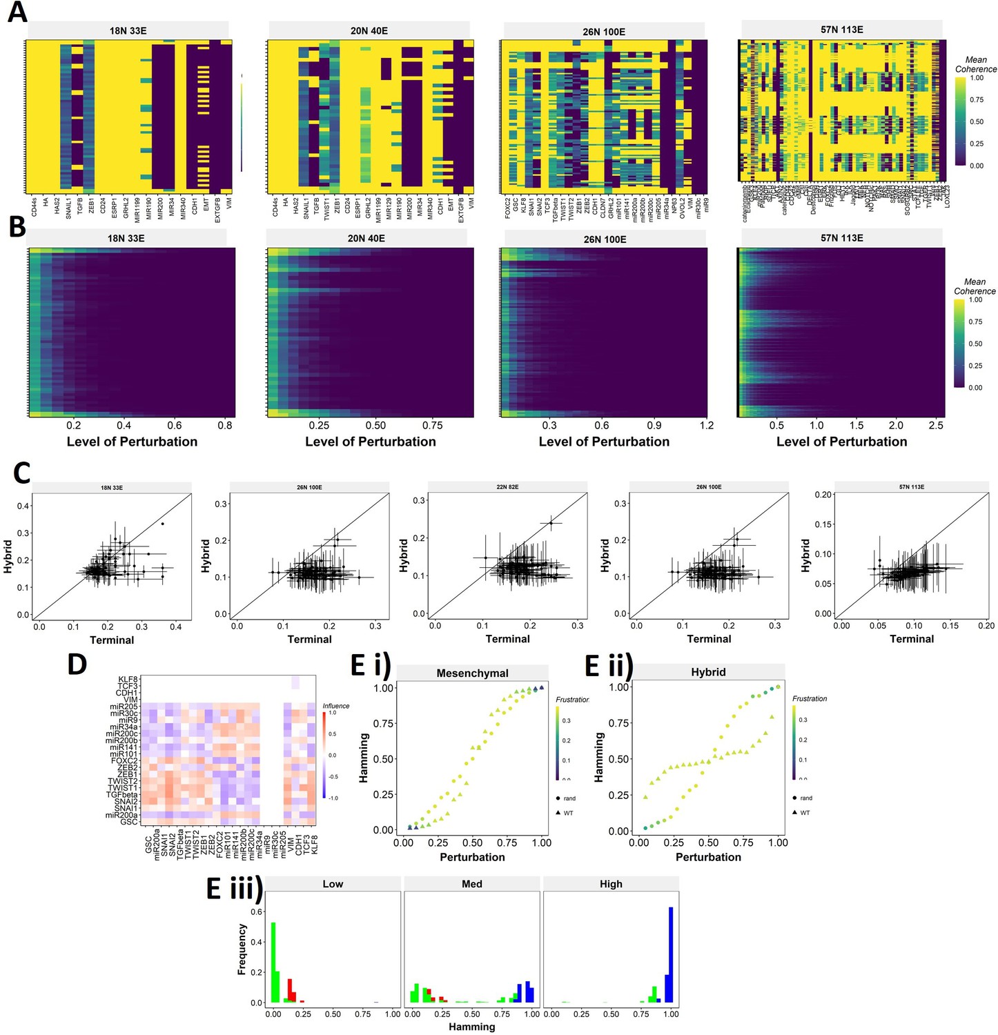
(A) Single-node perturbation coherence heatmaps for wild-type (WT) epithelial–mesenchymal plasticity (EMP) networks. (B) Multinode perturbation coherence heatmaps for WT EMP networks. (C) Half-minimum perturbation for terminal and hybrid states for the random networks. Each dot represents mean half-minimum perturbation for terminal and hybrid states for a network, and the bars represent standard deviation. (D) Influence matrix of the random network with low group strength taken as the representative case for Figure 6E (E) Representative cases of comparison of transition dynamics for (i) mesenchymal and (ii) hybrid steady states between WT and random network. (iii) Representative distribution of hamming distance for perturbation of hybrid phenotype.
Figure 6—figure supplement 2
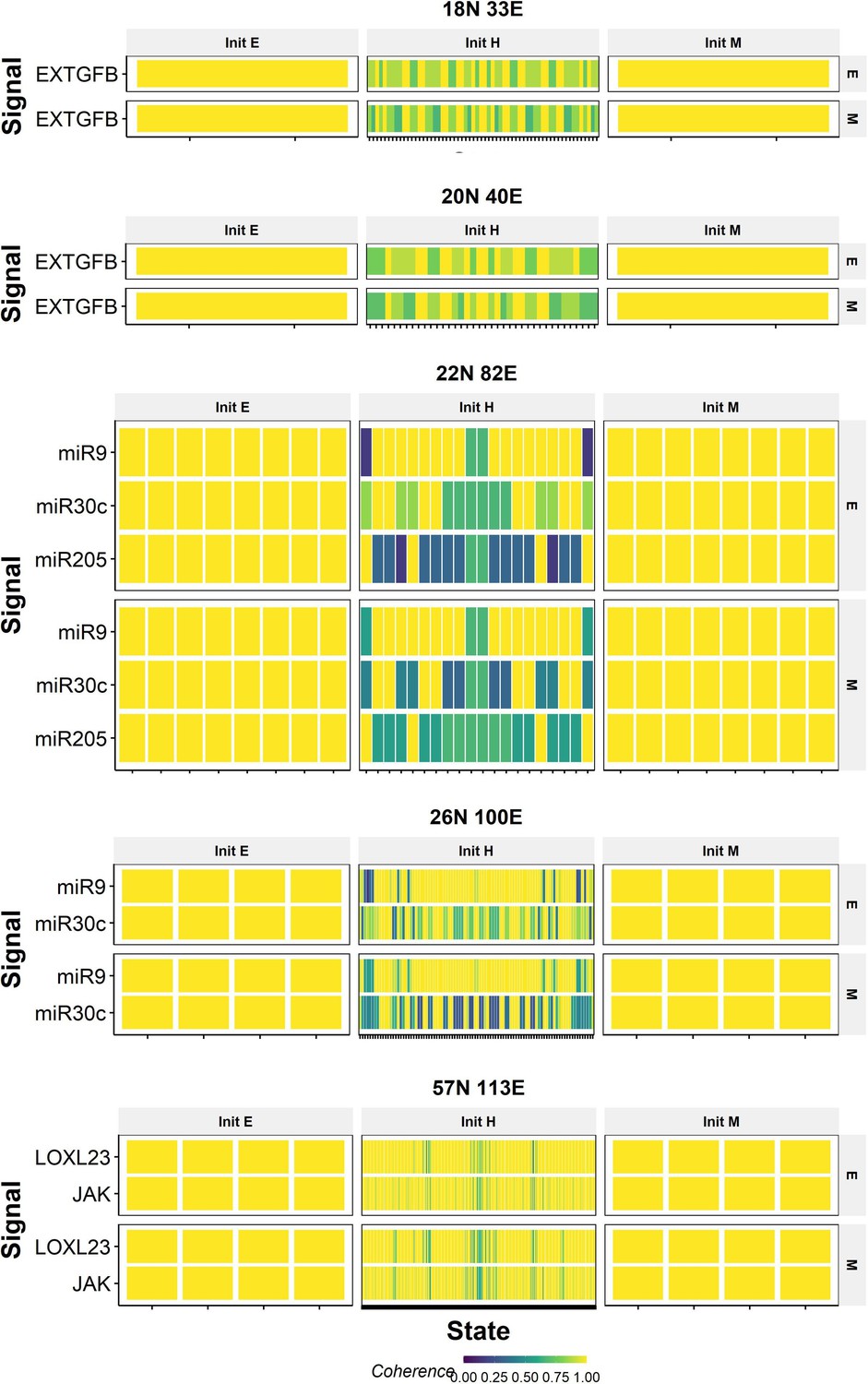
Coherence of calculated values for the core nodes upon perturbing signal nodes in wild-type (WT) epithelial–mesenchymal plasticity (EMP) networks.
Figure 7 with 1 supplement
Distinction between the transition dynamics of hybrid and terminal phenotypes is lost as teams weaken.
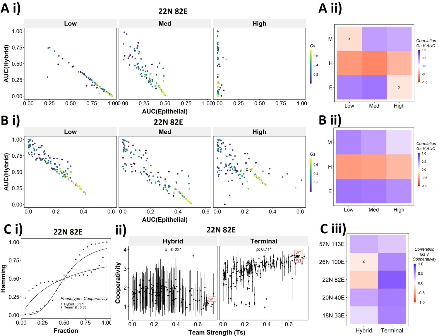
(A) (i) Scatterplot between mean area under the curve (AUC) of epithelial states and mean AUC of hybrid states when starting from epithelial phenotype. Each dot is a random network, colored by its team strength. (ii) Heatmap depicting the Spearman’s correlation between team strength and AUC for the final phenotype (y-axis) and the regions in the sigmoidal plot (x-axis). (B) Same as (A), but for hybrid as the starting phenotypes. (C) (i) Depiction of cooperativity with a terminal and hybrid state of the wild-type (WT) epithelial–mesenchymal plasticity (EMP) network 22N 82E. (ii) Team strength vs. cooperativity for random and WT networks of size 22N 82E. Each dot represents the mean cooperativity for one network. The bars show standard deviation. (iii) Correlation between team strength and cooperativity for random networks corresponding to WT EMP networks of different sizes.
Figure 7—figure supplement 1
Dependence of perturbation coherence on team strength.
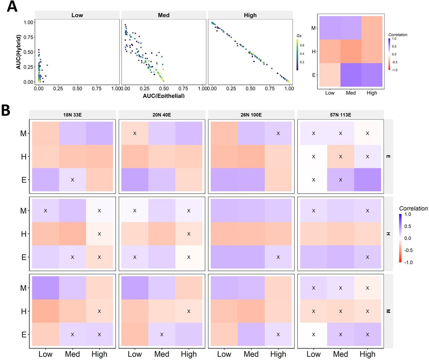
(A) Same as Figure 7A but for mesenchymal phenotype as the beginning. (B) Heatmaps depicting the correlation between mean group strength and area under the curve (AUC) for combinations of perturbation strengths (x-axis) and final phenotypes (y-axis) for all networks. The starting phenotypes are shown to the right.
Figure 8
Reducing team strength leads to reduction in terminal phenotype stability.
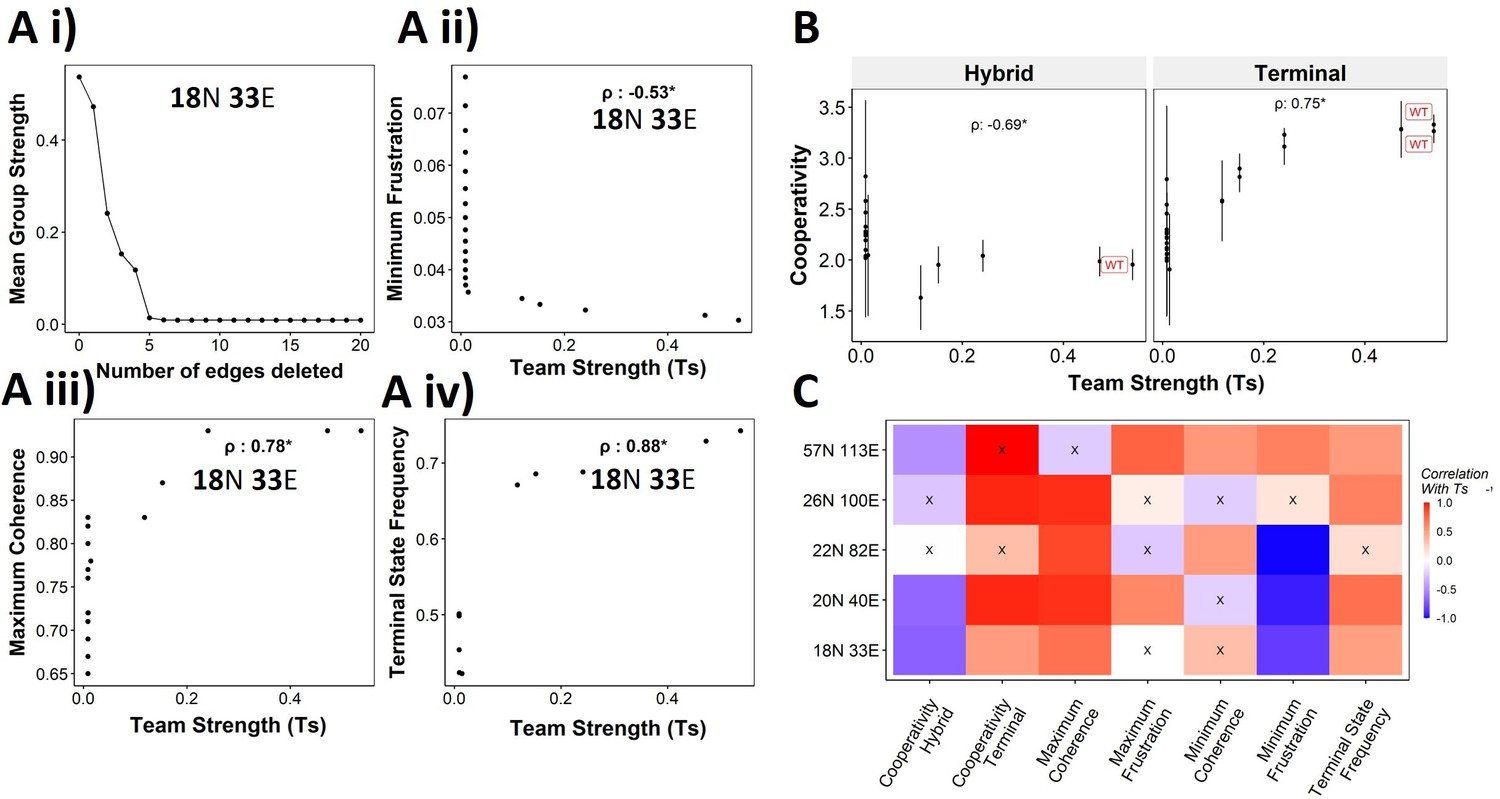
(A) (i) Lineplot to demonstrate the reduction of team strength with each edge perturbed. Change in (ii) minimum frustration, (iii) maximum coherence, and (iv) terminal state frequency with increase in team strength. (B) Mean cooperativity for the perturbed networks against the team strength. (C) Correlation between team strength and stability metrics for the perturbed networks (edge deleted one at a time sequentially as shown for 18N 33E network in panel A) obtained from all five epithelial–mesenchymal plasticity (EMP) networks.
Figure 9 with 1 supplement
Effect of teams on phenotypic landscape in small cell lung cancer (SCLC) and melanoma.
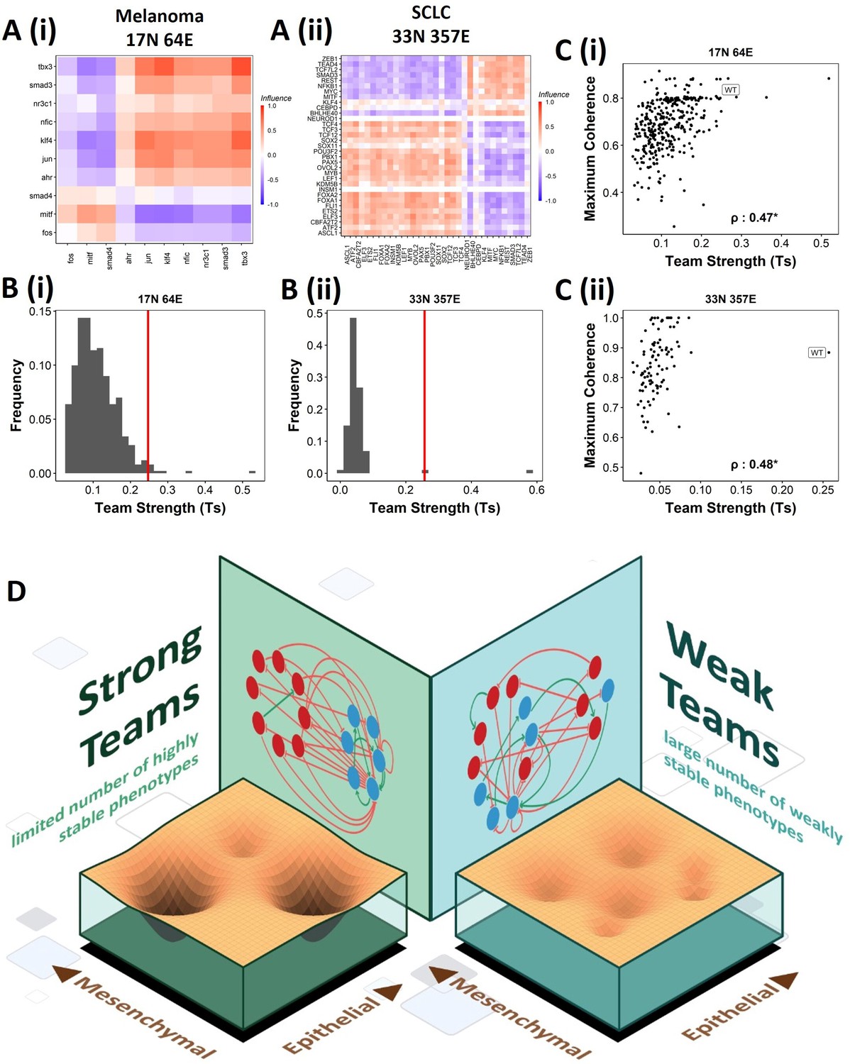
(A) Influence matrices of (i) melanoma (17N 64E) and (ii) SCLC (33N 357E) networks, depicting the two team structure observed. (B) Comparison of team strength distributions obtained for random networks corresponding to (i) melanoma and (ii) SCLC, with the wild-type (WT) melanoma and SCLC team strengths labeled by red vertical line. (C) Scatterplots depicting the maximum coherence against the team strength of the random networks corresponding to (i) melanoma and (ii) SCLC. Spearman’s correlation coefficient reported. *p<0.05. (D) Schematic showing the effect of team structure on the phenotypic stability landscape emergent from the network topology.
Figure 9—figure supplement 1
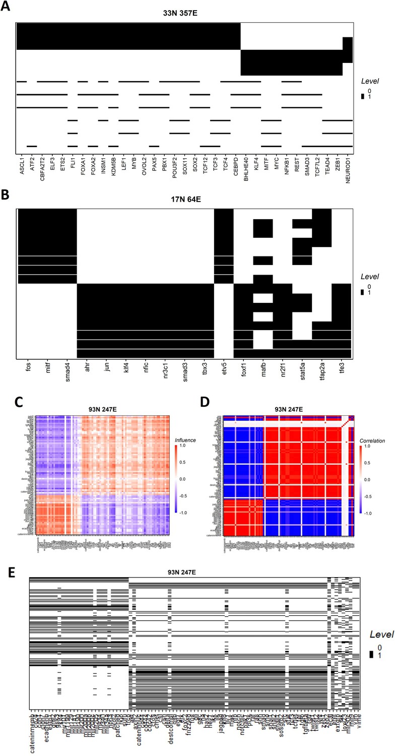
SSF and correlation analysis of non-EMP netowrks.
(A, B) Heatmaps showing the steady-state composition and the corresponding steady-state frequency (SSF) of (A) small cell lung cancer (SCLC) and (B) melanoma Gene Regulatory Netowrks. Each row represents a state and each column a node. The height of each row represents the SSF of that state. (C) Influence matrix of the combined epithelial–mesenchymal plasticity (EMP) network. (D) Correlation matrix of the combined EMP network obtained from Boolean simulations. (E) Same as (A, B), but for the combined EMP network.
Tables
Appendix 1—table 1
Parameter ranges for RACIPE simulations.
| Parameters | Minimum | Maximum |
|---|---|---|
| Production rate (G) | 1 | 100 |
| Degradation rate (k) | 0.1 | 1 |
| Fold Change (Inhibition λ) | 0.01 | 1 |
| Fold Change (Activation λ) | 1 | 100 |
| Hill coefficient | 1 | 6 |
| Threshold | The ranges depend on inward | regulation - half functional rule |
Additional files
Download links
A two-part list of links to download the article, or parts of the article, in various formats.
Downloads (link to download the article as PDF)
Open citations (links to open the citations from this article in various online reference manager services)
Cite this article (links to download the citations from this article in formats compatible with various reference manager tools)
Landscape of epithelial–mesenchymal plasticity as an emergent property of coordinated teams in regulatory networks
eLife 11:e76535.
https://doi.org/10.7554/eLife.76535


