Mapping circuit dynamics during function and dysfunction
- Volen Center and Biology Department, Brandeis University, United States
- Federated Department of Biological Sciences, New Jersey Institute of Technology and Rutgers University, United States
Figures
Figure 1
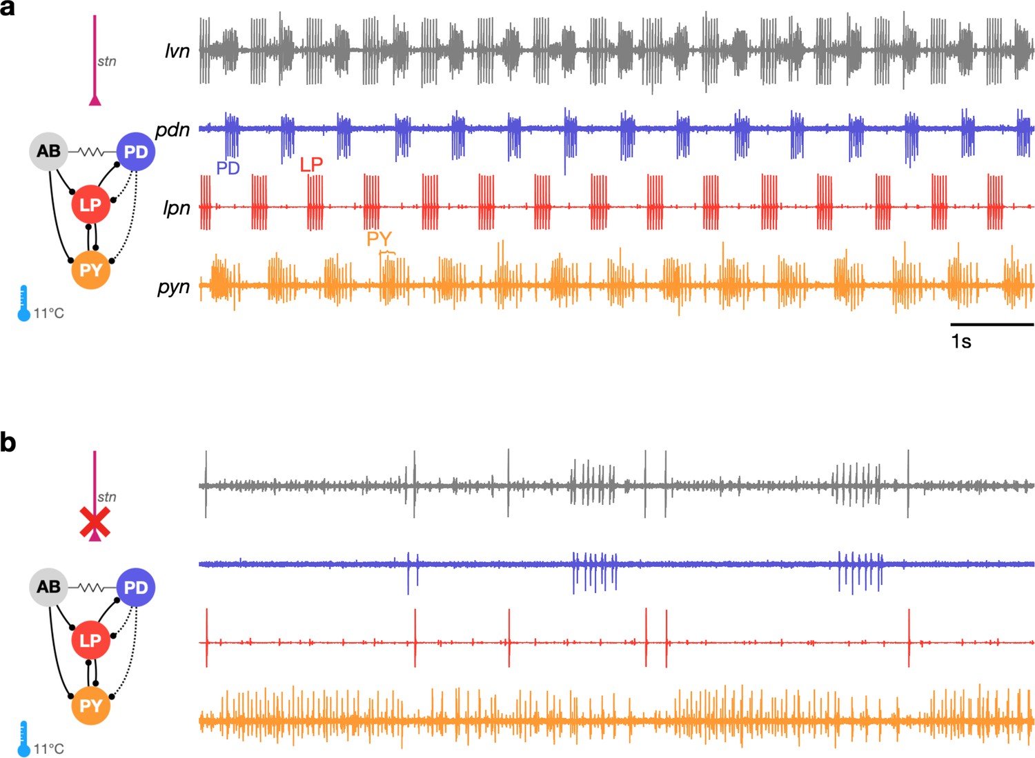
The triphasic pyloric rhythm can become irregular and hard to characterize under perturbation.
(a) Simplified schematic of part of the pyloric circuit (left). Filled circles indicate inhibitory synapses, solid lines are glutamatergic synapses, and dotted lines are cholinergic synapses. Resistor symbol indicates electrical coupling. The pyloric circuit is subject to descending neuromodulatory control from the stomatogastric nerve (stn). Right: simultaneous extracellular recordings from the lvn, lpn, pdn, and pyn motor nerves. Action potentials from lateral pyloric (LP), pyloric dilator (PD), and pyloric (PY) are visible on lpn, pdn, and pyn. Under these baseline conditions, PD, LP, and PY neurons burst in a triphasic pattern. The anterior burster (AB) neuron is an endogenous burster and is electrically coupled to PD neurons. (b) When the stn is cut, neuromodulatory input is removed and the circuit is ‘decentralized.’ In this case, the pyloric rhythm can become irregular and hard to characterize. In addition, spikes from multiple PY neurons can become harder to reliably identify on pyn.
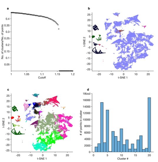
Figure 2 with 5 supplements
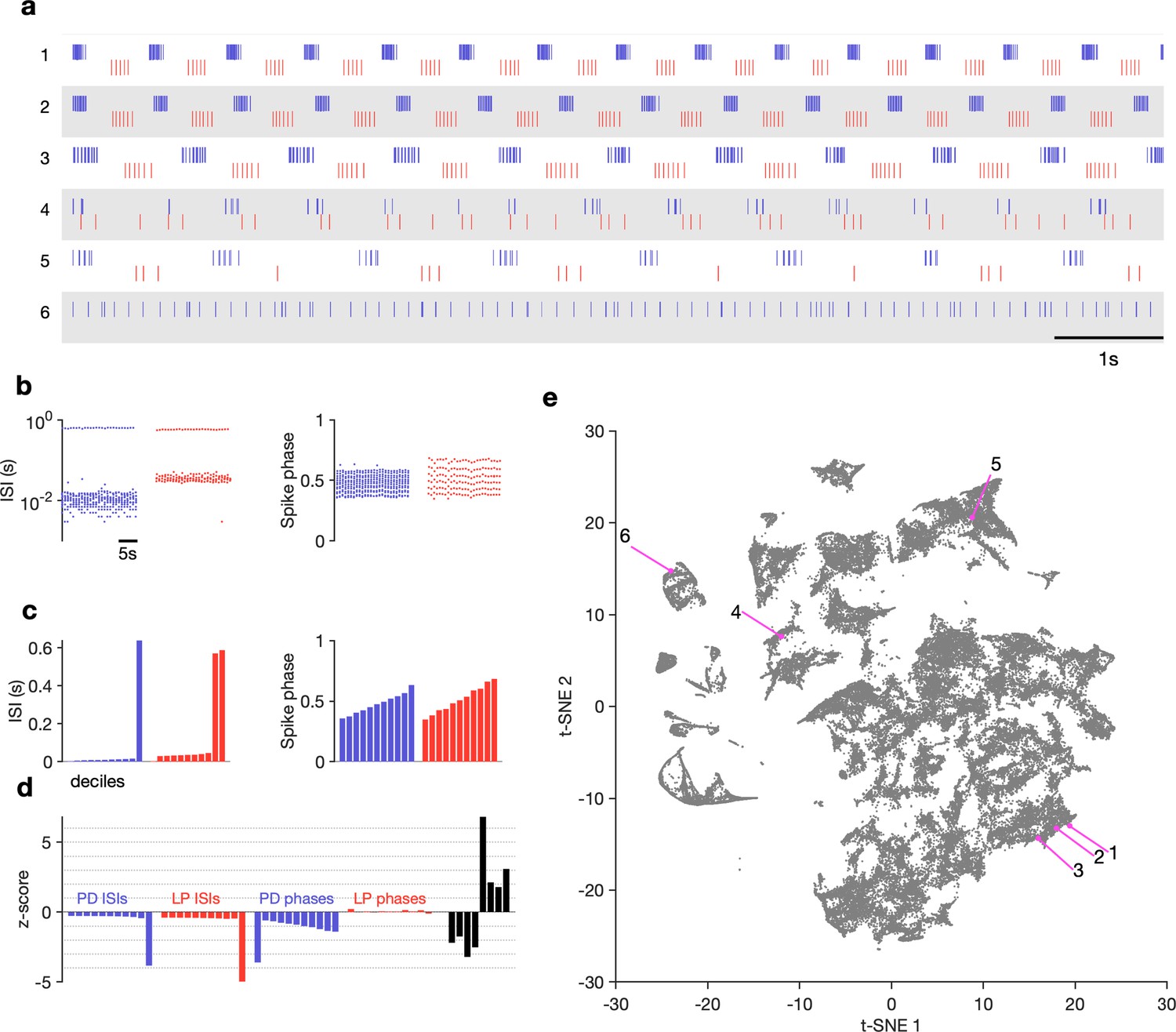
Visualization of diverse neural circuit dynamics.
(a) Examples of canonical (1–3) and atypical (4–6) spike patterns of pyloric dilator (PD; blue) and lateral pyloric (LP; red) neurons. Rasters show 10 s of data. (b–d) Schematic of data analysis pipeline. (b) Spike rasters in (a2) can be equivalently represented by interspike intervals (ISIs) and phases. 20 s bins shown. Each 20 s bin contains a variable number of spikes/ISIs. (c) Summary statistics of ISI and phase sets in (d), showing tenth percentiles. Using percentiles converts the variable length sets in (b) to vectors of fixed length. (d) -scored data assembled into a single vector, together with some additional measures (Materials and methods). (e) Embedding of data matrix containing all vectors such as the one shown in (d) using t-distributed stochastic neighbor embedding (t-SNE). Each dot in this image corresponds to a single 20 s spike train from both LP and PD. Example spike patterns shown in (a) are highlighted in the map. points from animals. In (a–d), features derived from LP spike times are shown in red, and features derived from PD spike times are shown in blue.
Figure 2—figure supplement 1
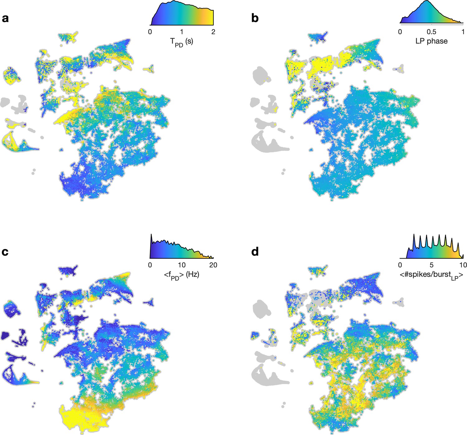
Burst metrics smoothly vary in map.
In each panel, embedding of the entire dataset is shown in gray. Points are colored by (a) burst period of the pyloric dilator (PD) neuron (b) phase of lateral pyloric (LP) burst start in PD time (c) mean firing rate of PD neuron, and (d) mean number of spikes per burst in the LP neuron. In each panel, the color scale also shows the distribution of metric over the entire dataset (y-axis in log scale). The distribution in (d) is spiky because the mean number of spikes/burst tends to be integer valued.
Figure 2—figure supplement 2
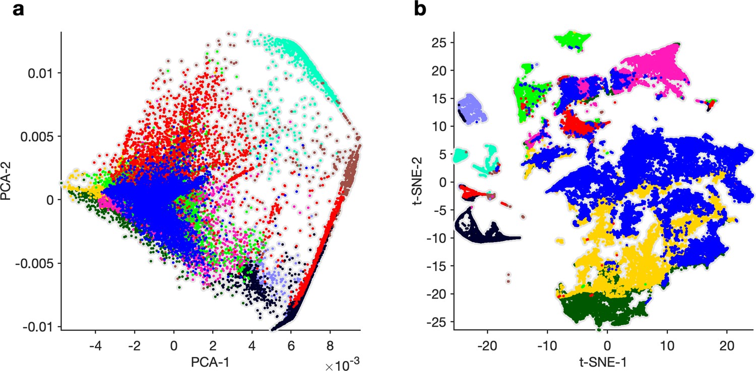
Principal components analysis (PCA) and k-means to find clusters in feature vectors.
(a) First and second components of PCA of feature vectors. Each dot is a single 20 s spike pattern from both pyloric dilator (PD) and lateral pyloric (LP) neurons. Colors correspond to cluster IDs from k-means on the first 10 principal components. (b) Cluster indices from (a) used to color points in the t-distributed stochastic neighbor embedding (t-SNE) embedding. The PCA + k-means approach tends to split up the large regular cluster, and clusters from k-means span clusters in t-SNE space, which were subsequently found to include spike patterns that were qualitatively different.
Figure 2—figure supplement 3
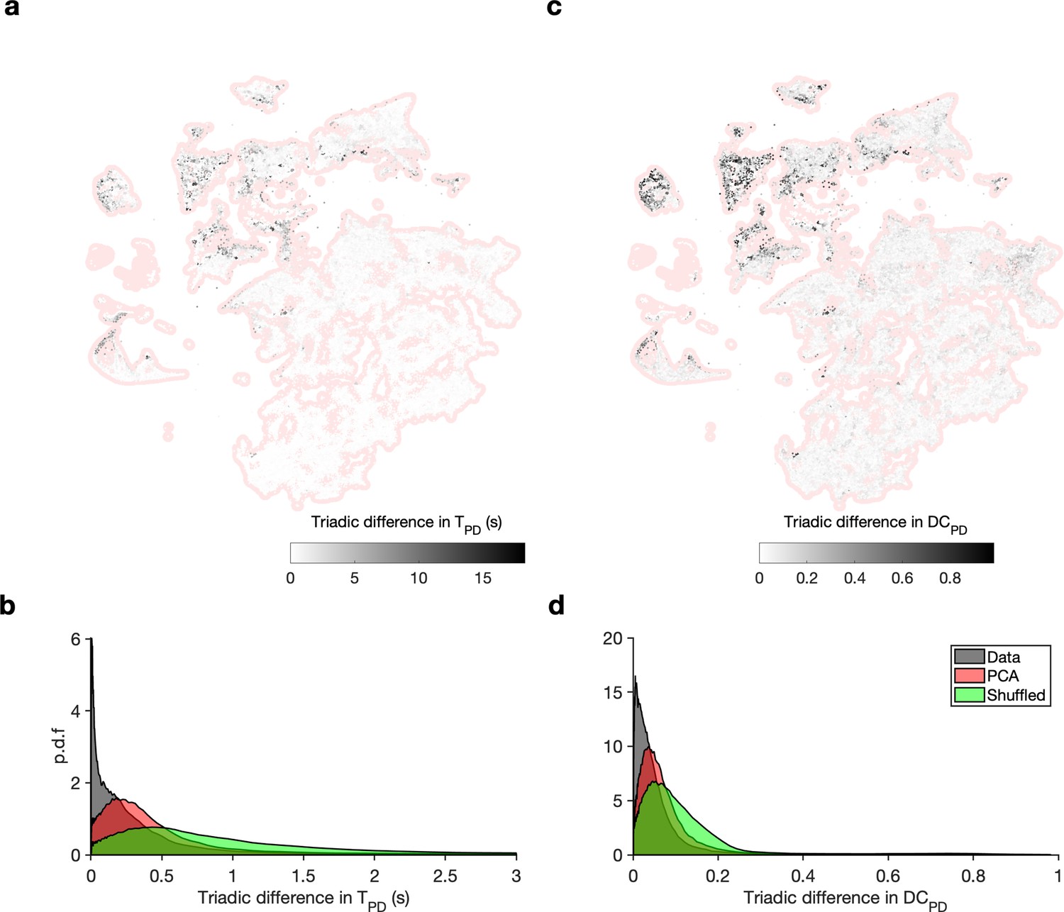
Embedding arranges data so that neighbors tend to be similar.
(a) Map shows embedding of all data in red shading. Shaded dots are incenters of a Delaunay triangulation of the map, and shading indicates the maximum absolute value of difference between burst period of the pyloric dilator (PD) neuron in each cell in the triangulation. (b) Distribution of absolute triadic differences over the entire dataset (gray) compared to triadic differences between shuffled triads (green) and compared to triadic differences between the first two principal components. Triadic differences are significantly smaller than in the shuffled data and in the principal components (p<0.001, Kolmogorov–Smirnov test). (c, d) Same as in (a, b), for the duty cycle of the PD neuron.
Figure 2—figure supplement 4
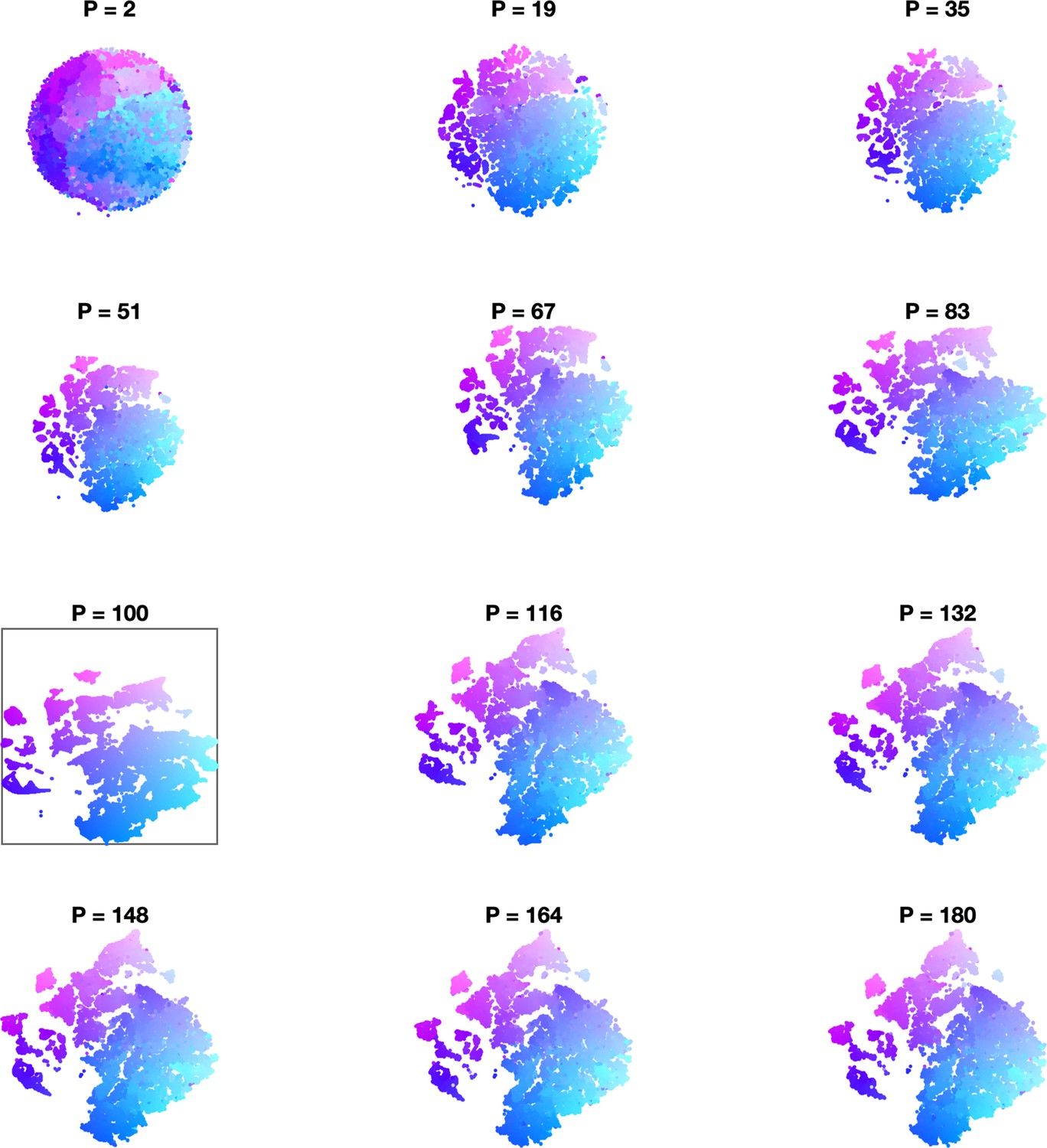
Effect of varying perplexity in t-distributed stochastic neighbor embedding (t-SNE) embedding.
In each panel, data are embedded using t-SNE using the indicated perplexity parameter. Initialization is the same across all perplexities (Materials and methods). In every panel, points are colored by their location in the embedding with (black box).
Figure 2—figure supplement 5
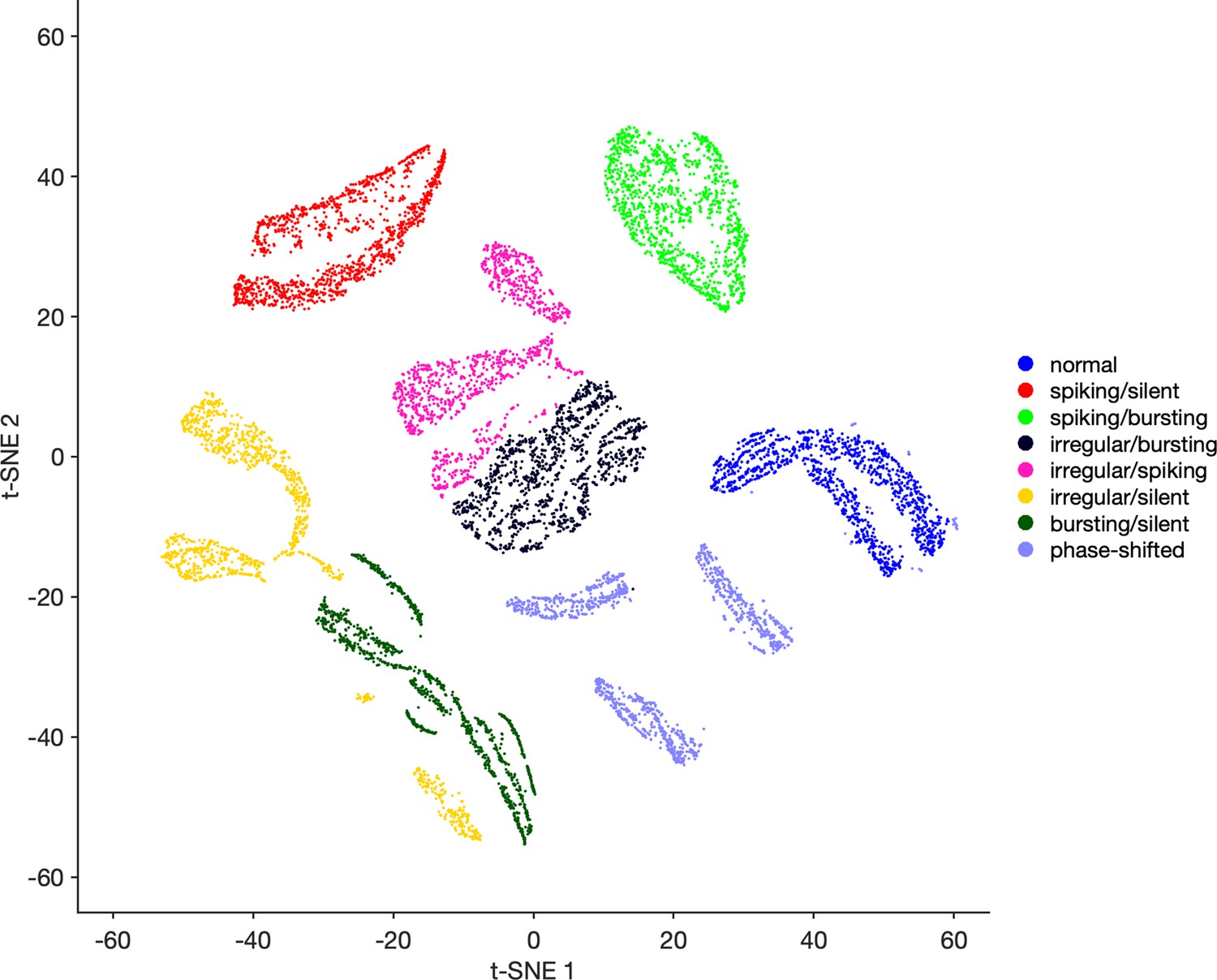
Validation of method using synthetic data.
Synthetic data with different spike pattern classes converted into feature vectors and embedded using t-distributed stochastic neighbor embedding (t-SNE) as described (Materials and methods). Data from different classes tend to be well separated in the map, suggesting that this method can identify stereotyped and distinct spike patterns in neural recordings.
Figure 3 with 3 supplements
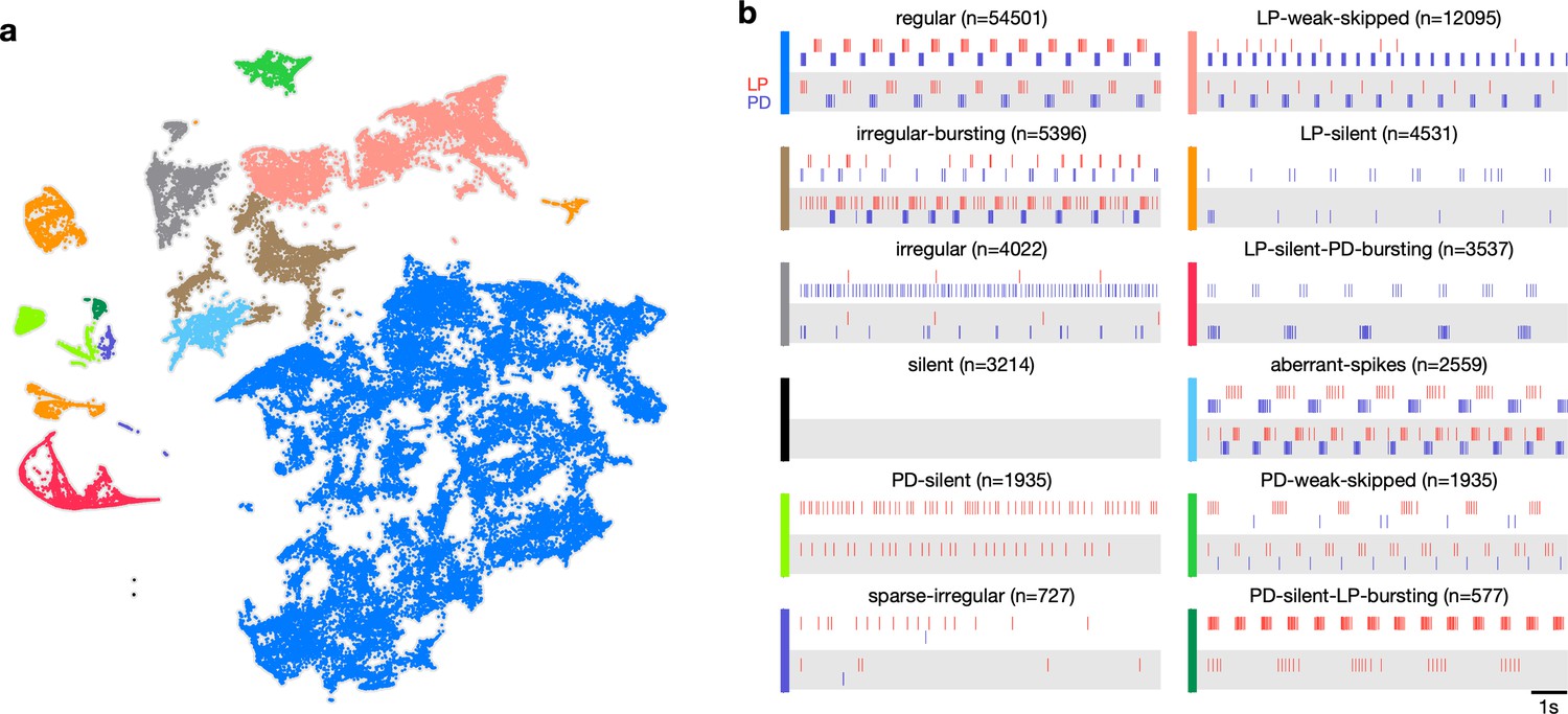
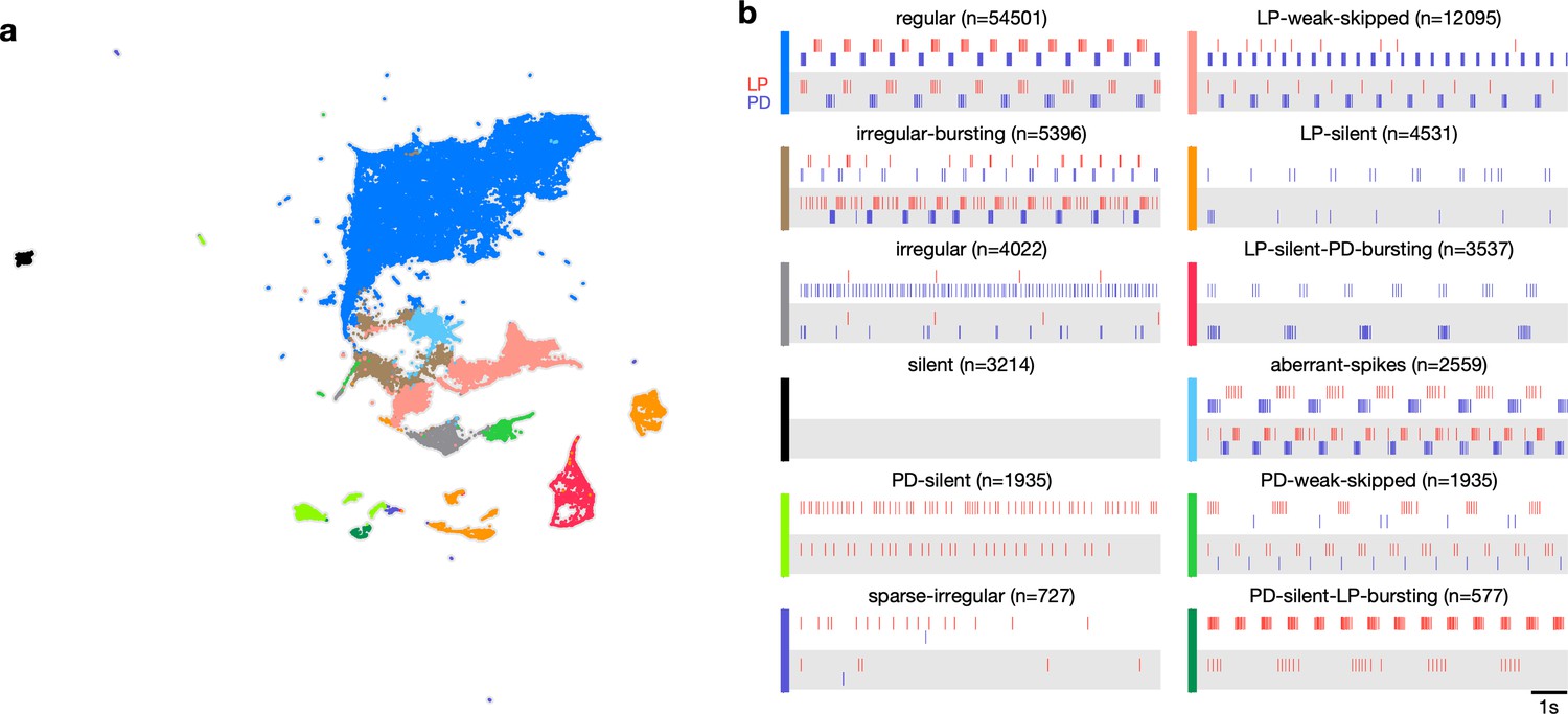
Map allows identification of distinct spiking dynamics.
(a) Map of all pyloric dynamics in dataset where each point is colored by manually assigned labels. Each point corresponds to a 20 s paired spike train from lateral pyloric (LP) and pyloric dilator (PD) neurons. Each panel in (b) shows two randomly chosen points from that class. The number of points in each class is shown in parentheses above each panel. points from animals. Labels are ordered by likelihood in the data.
Figure 3—figure supplement 1
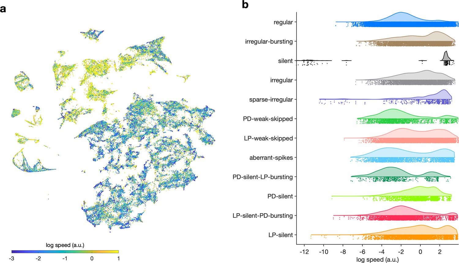
Speed of trajectories through map.
(a) Map colored by speed of trajectories through map at that point. Cooler colors indicate that preparations move through that region of space more slowly, and warmer colors suggest that preparations are more likely to be far from that location in the next time step. (b) Speed grouped by manually identified labels.
Figure 3—figure supplement 2
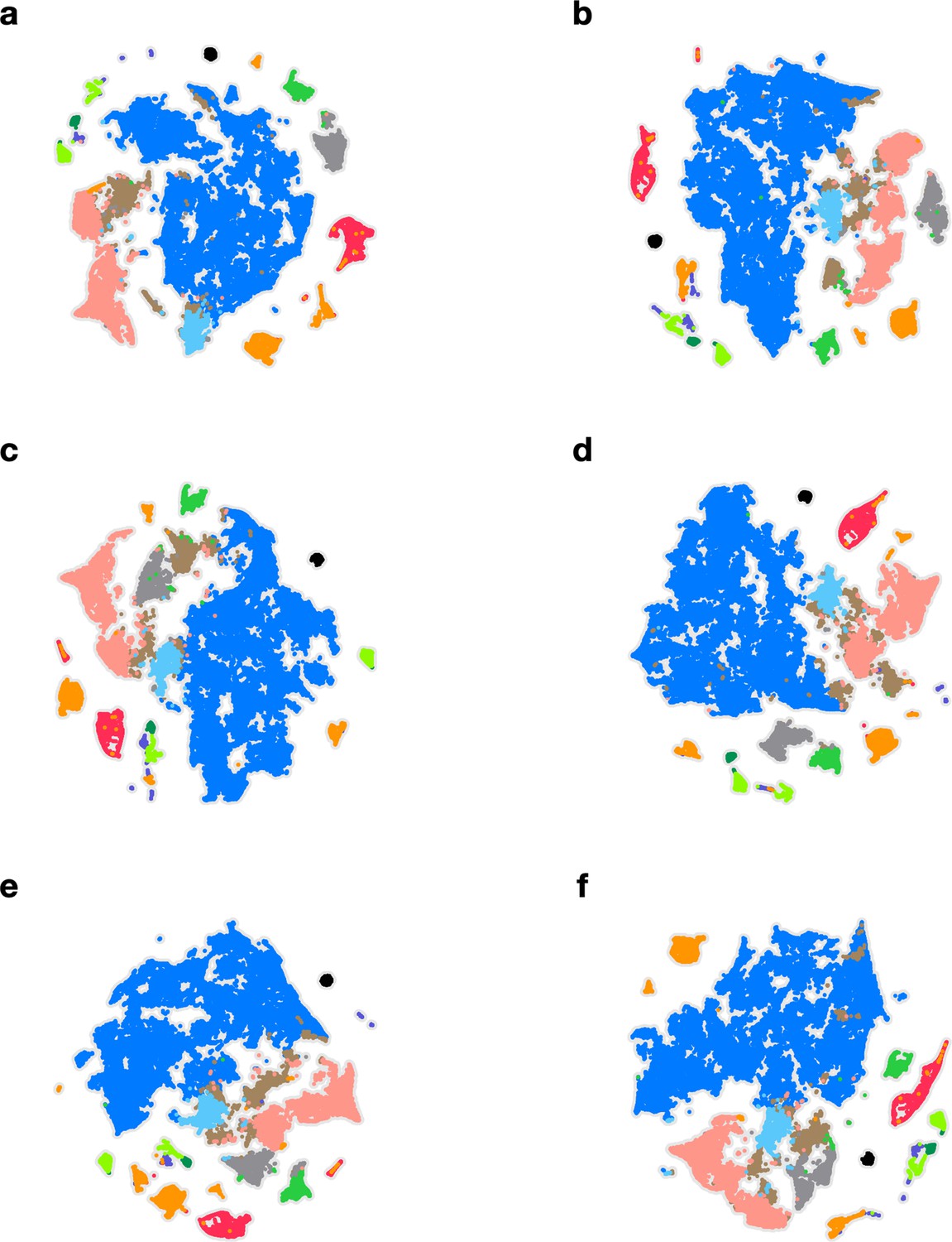
Embeddings with different initializations.
In each panel, the embedding is performed with a different initialization. (a–d) Random initializations. (e) Initializations based on minimum interspike intervals (ISIs) in pyloric dilator (PD) and lateral pyloric (LP) neurons. (f) Initializations based on mean ISIs in PD and LP neurons. In every panel, points are colored identically.
Figure 3—figure supplement 3
Using Uniform Manifold Approximation and Projection (uMAP) instead of t-distributed stochastic neighbor embedding (t-SNE).
Instead of t-SNE, we used uMAP to embed the feature vectors in two dimensions (a). Points are colored identically to Figure 3. The coarse features of the map are preserved here, even though we used a different embedding algorithm. Each panel in (b) shows two randomly chosen points in that class.
Figure 4 with 3 supplements

Variability of burst metrics under baseline conditions.
(a) Variability of burst metrics in pyloric dilator (PD) and lateral pyloric (LP) neurons across a population of wild-caught animals. Metrics are only computed under baseline conditions and in the regular cluster. (b) Distribution of coefficient of variation (CV) of metrics in each animal across all data from that animal. In (a, b), each dot is from a single animal, and distributions show variability across the entire population. (c) Across-animal variability (CV of individual means, Δ) is greater than within-animal variation (mean of CV in each animal, Ο) for every metric. (d) Difference between across-animal variability and within-animal variability (colored dots). For each metric, gray dots and distribution show differences between across-animal and within-animal variability for shuffled data. points from animals.
Figure 4—figure supplement 1
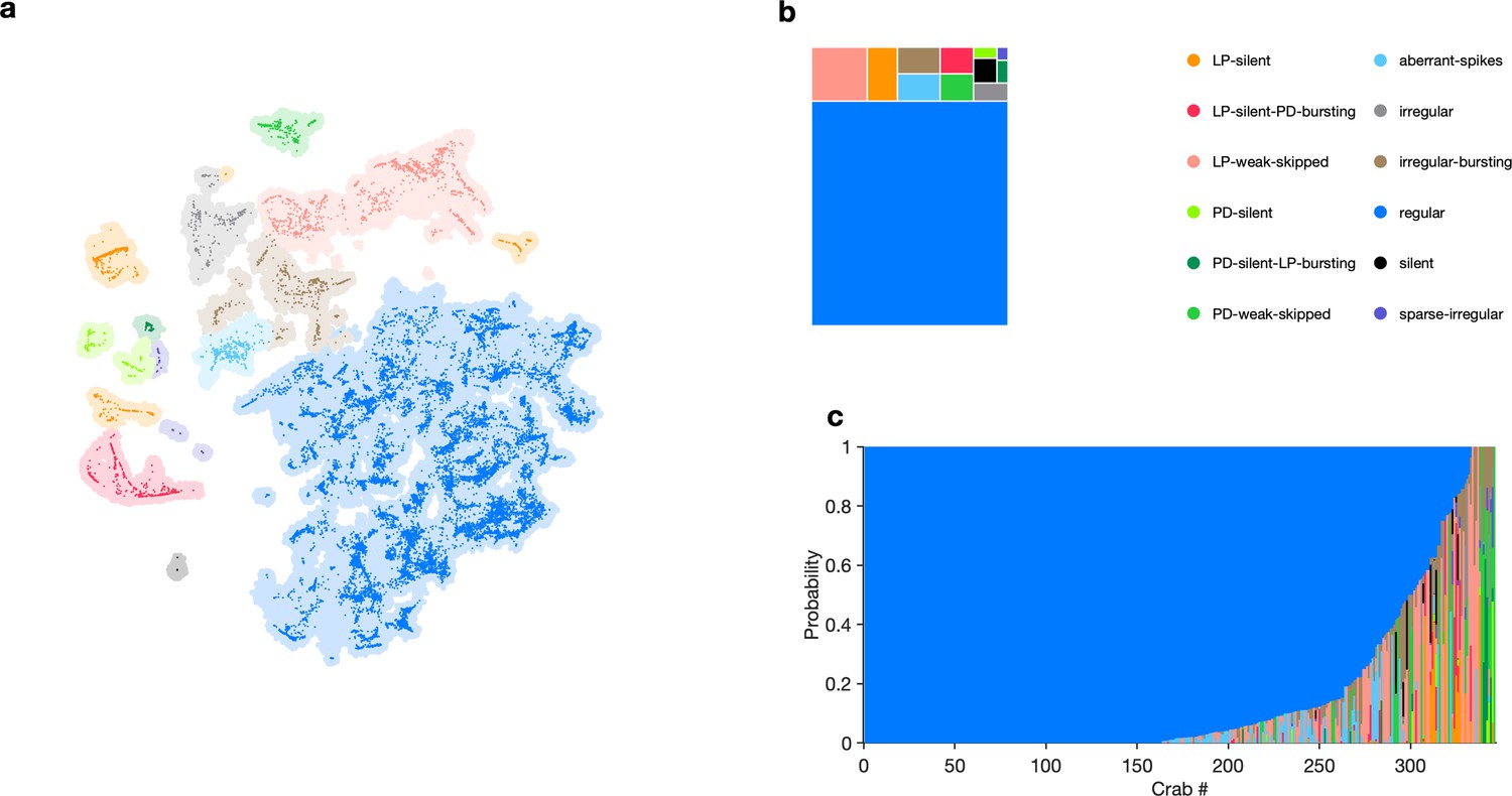
State distribution under baseline conditions.
(a) Map showing occupancy of baseline data. Shading indicates all data. Bright colored points are data from baseline conditions. (b) Treemap showing state probabilities under baseline conditions. (c) Preparation-by-preparation variation in state distribution under baseline conditions. data snippets from individual preparations.
Figure 4—figure supplement 2
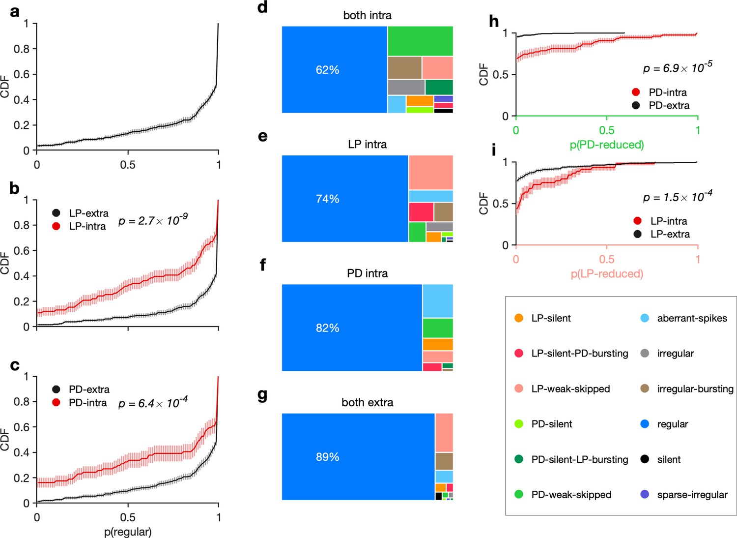
Recording condition alters regular state probability.
(a) Cumulative probability of the probability of observing a regular state, per animal. Cumulative probability of probability of regular state for preparations with lateral pyloric (LP) (b) and pyloric dilator (PD) (c) neurons recorded extracellularly (black) vs. LP recorded intracellularly (red). (d–g) State probabilities in different recording conditions. (h) Probability of observing states in which PD activity is reduced (PD-silent, PD-weak-skipped) in preparations in which PD is recorded intracellularly (red) vs. preparations in which PD is recorded extracellularly (black). (i) Same as (h), but for LP. In all panels, thick lines show CDFs and shading indicates confidence intervals estimated by bootstrap. , N = 346. p-values in each panel are from two-sample Kolmogorov-Smirnov tests.
Figure 4—figure supplement 3
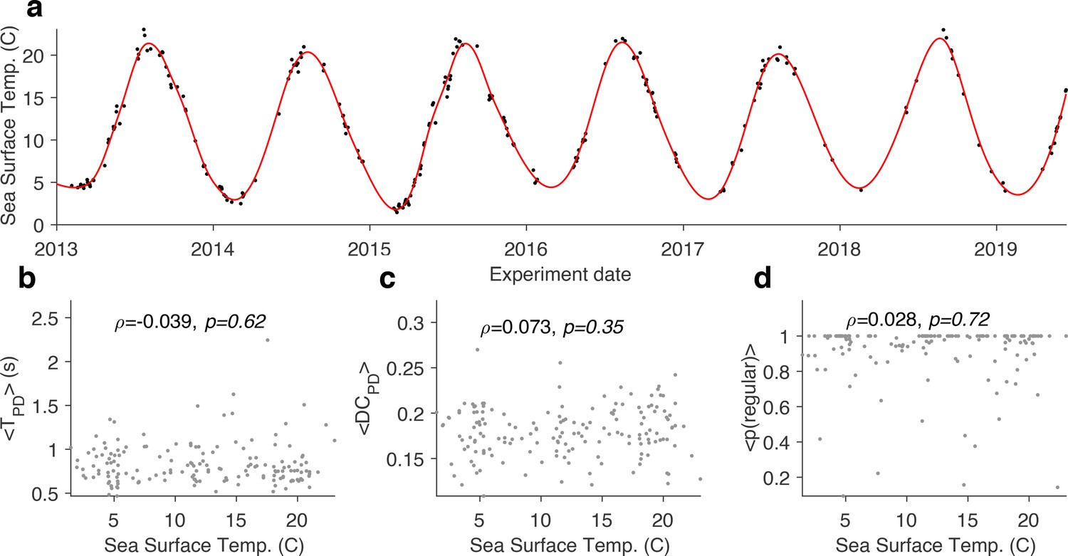
Effect of sea surface temperature on baseline circuit dynamics.
(a) Sea surface temperature at the Boston Harbor vs. experimental date. Red line is a smoothing fit. Mean burst period of pyloric dilator (PD) neuron (b), mean duty cycle of PD (c), and probability of observing the regular state (d) vs. sea surface temperature. In all panels, each dot corresponds to a single preparation. preparations. is the Spearman correlation coefficient, and -value is from the Spearman rank correlation test.
Figure 5 with 1 supplement
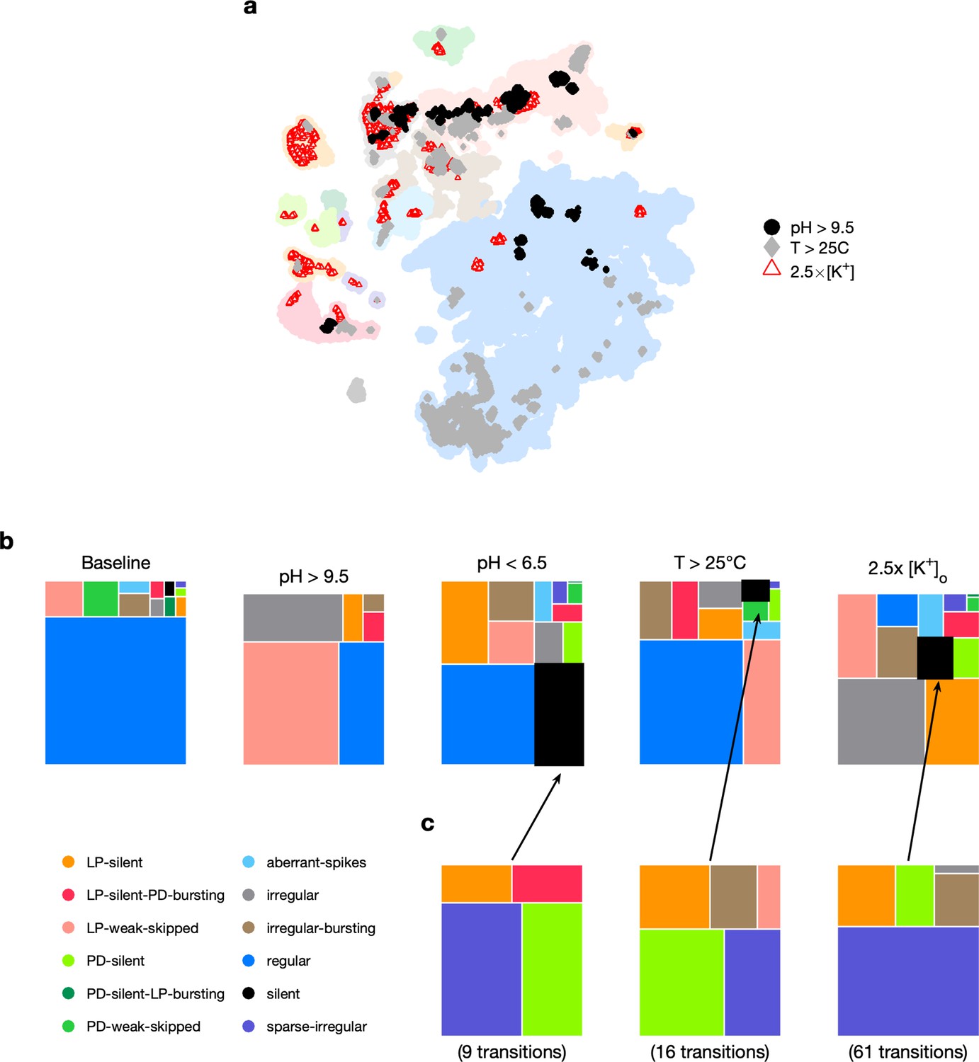
Effect of three different environmental perturbations.
(a) Map showing regions that are more likely to contain data recorded under extreme environmental perturbations. (b) Treemaps showing probability distributions of states under baseline and perturbed conditions. (c) Probability distribution of states preceding silent state under perturbation. pH perturbations: from 6 animals; perturbations: from 20 animals; temperature perturbations: from 414 animals.
Figure 5—figure supplement 1
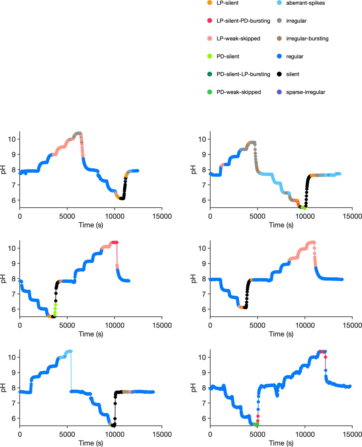
Preparation-by-preparation response to pH perturbations.
Each panel shows the response of a single preparation to pH perturbations. States are indicated in colors. Each preparation was stepped through various pH levels before returning to baseline pH. Note silent states (black) during acidic pH.
Figure 6
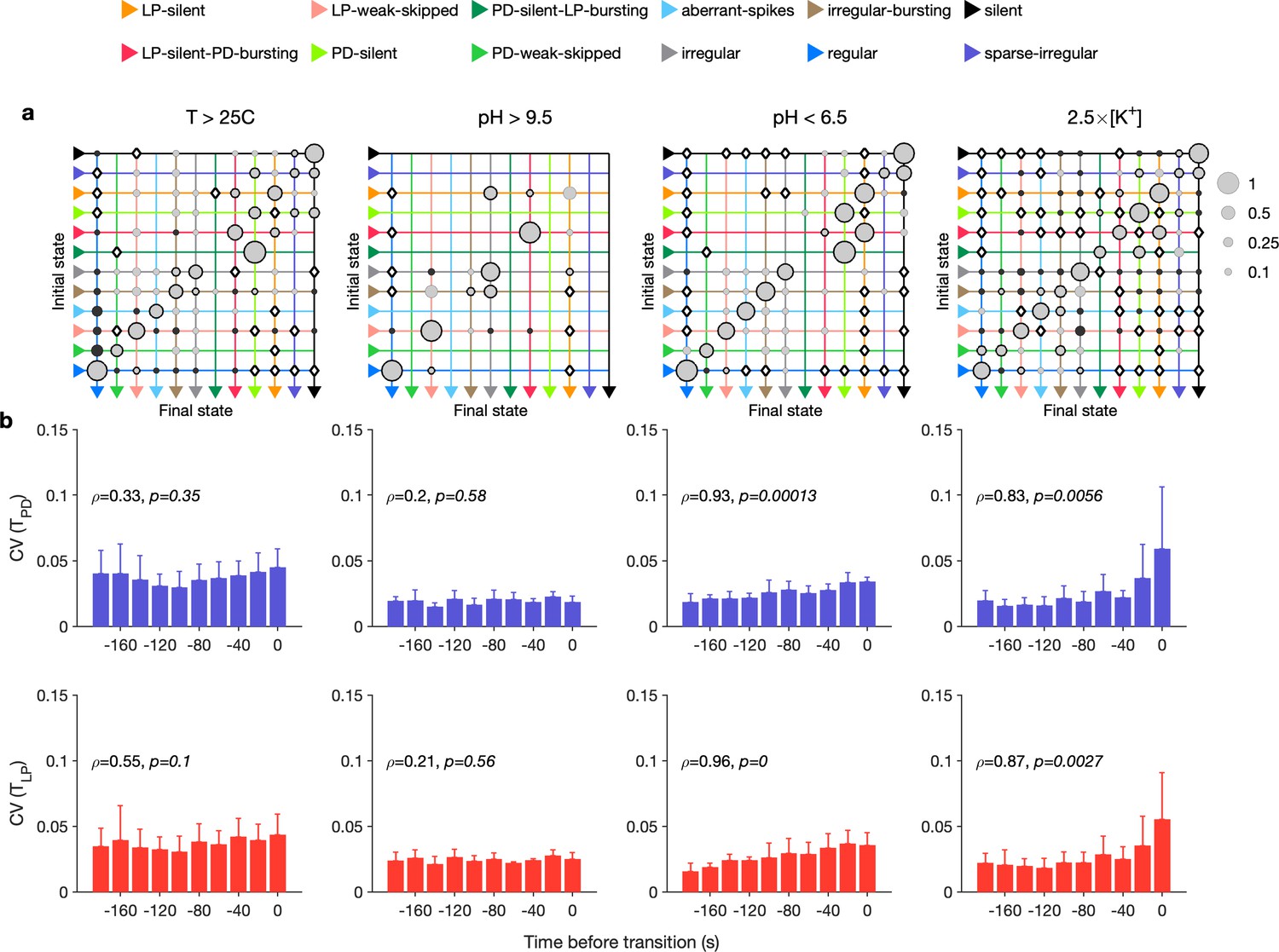
Effect of environmental perturbations on transitions between states.
(a) Transition matrix between states during environmental perturbations. Each matrix shows the conditional probability of observing the final state in the next time step given an observation of the initial state. Probabilities in each row sum to 1. Size of disc scales with probability. Discs with dark borders are transitions that are significantly more likely than the null model (Materials and methods). Dark solid discs are transitions with nonzero probability that are significantly less likely than in the null model. are transitions that are never observed and are significantly less likely than in the null model. States are ordered from regular to silent. (b) Coefficient of variation (CV) of burst period of pyloric dilator (PD) (purple) and lateral pyloric (LP) (red) vs. time before transition away from the regular state. are from Spearman test (on binned data, as plotted) to check if variability increases significantly before transition. Temperature perturbations: transitions in 61 animals; pH perturbations: transitions in 6 animals; perturbations: transitions in 20 animals.
Figure 7 with 4 supplements
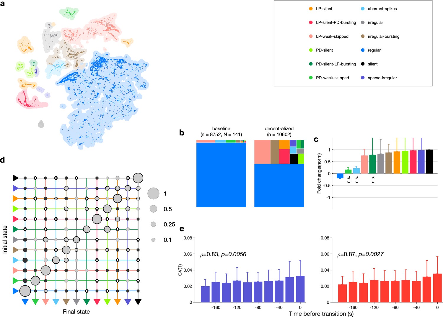
Effect of decentralization.
(a) Map occupancy conditional on decentralization. Shading shows all data, and bright colored dots indicate data when preparations are decentralized. (b) State probabilities before and after decentralization. (c) Fold change in state probabilities on decentralization. States marked n.s. are not significantly more or less likely after decentralization. All other states are (paired permutation test, p<0.00016). (a, b) points from animals. (d) Transition matrix during decentralization. Probabilities in each row sum to 1. Size of disc scales with probability. Discs with dark borders are transitions that are significantly more likely than the null model (Materials and methods). Dark solid discs are transitions with nonzero probability that are significantly less likely than in the null model. are transitions that are never observed and are significantly less likely than in the null model. States are ordered from regular to silent. transitions. (e) Coefficient of variation of pyloric dilator (PD, purple) and lateral pyloric (LP; red) burst periods before transition away from regular states. from Spearman test. points from animals.
Figure 7—figure supplement 1
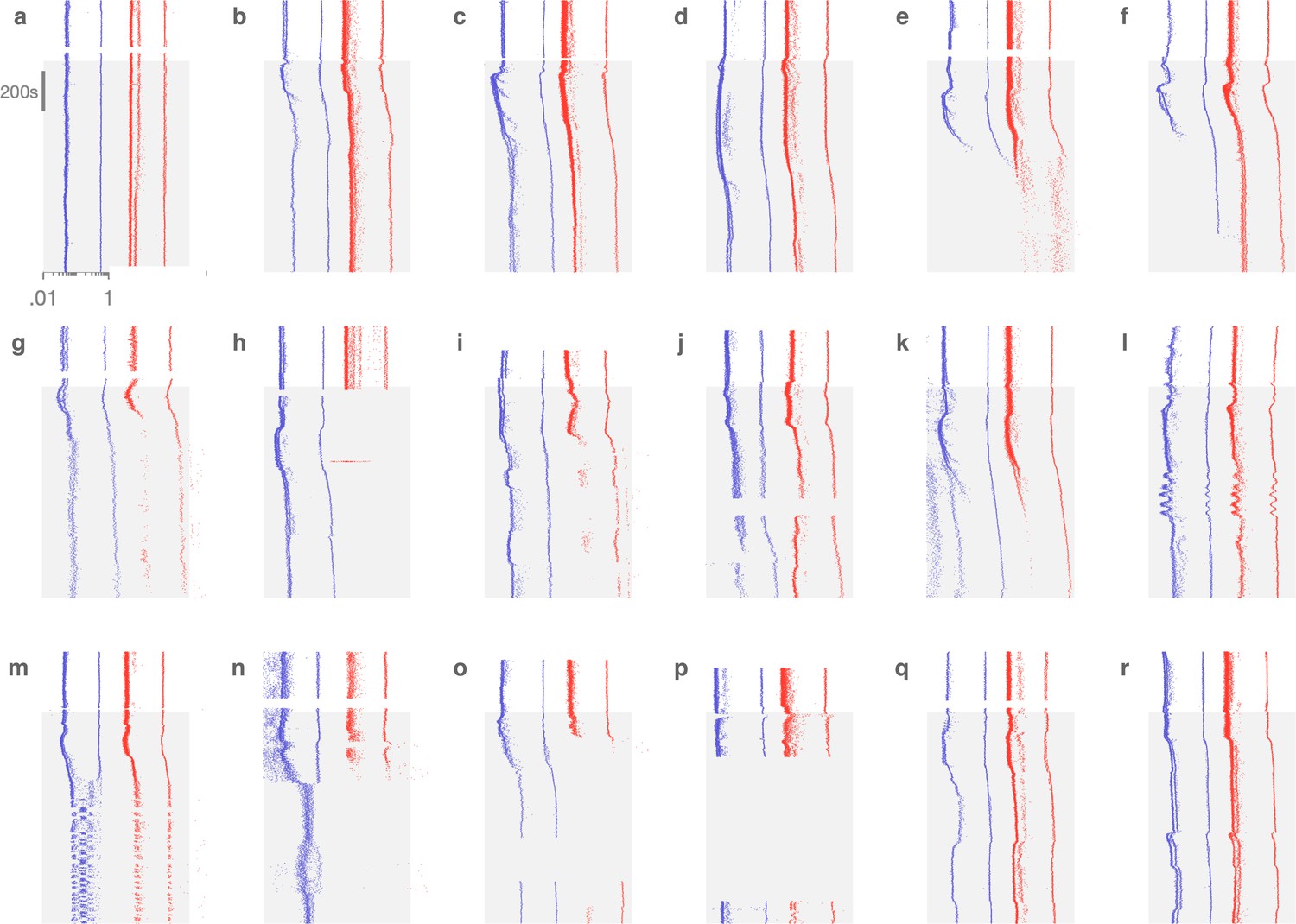
Decentralization evokes variable dynamics.
In each panel, interspike intervals (ISIs) of pyloric dilator (PD; blue) and lateral pyloric (LP; red) neurons are shown before and after (shaded) decentralization. The diversity of circuit responses to decentralization includes minimal change (a), transient perturbation followed by recovery (b–d), silence in one or two neurons (e–h), slow oscillatory responses (l), and a switch from bursting to spiking (m, n). Each panel corresponds to a different preparation.
Figure 7—figure supplement 2
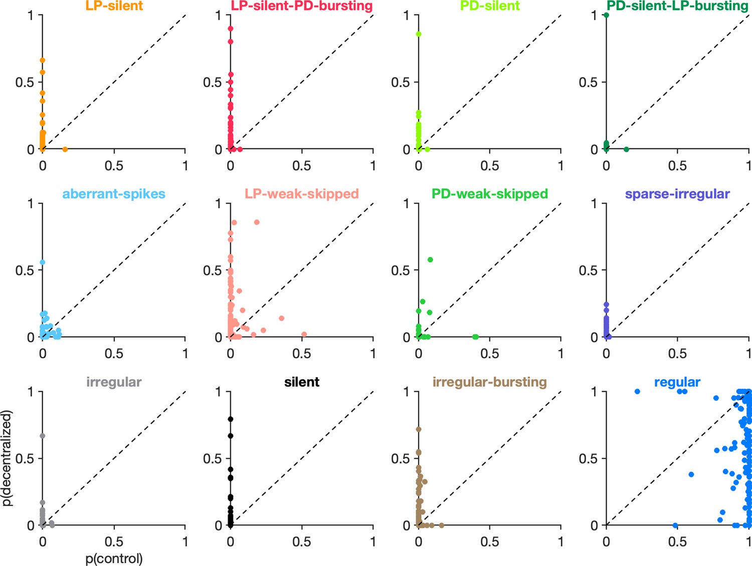
Effects of decentralization on state probabilities.
Each panel shows the probability of observing a given state before (x-axis) and after (y-axis) decentralization. Each dot is a single preparation. Probabilities computed on an animal-by-animal basis from points from preparations.
Figure 7—figure supplement 3
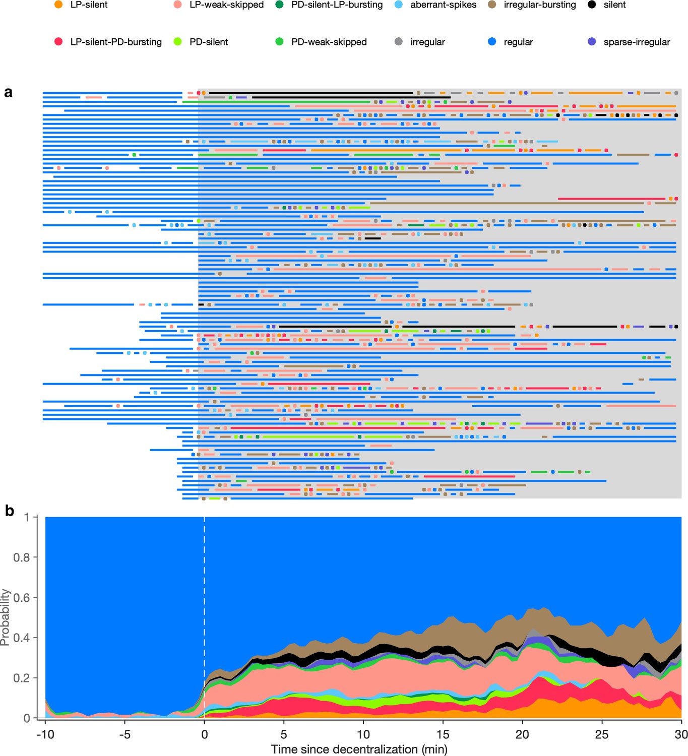
Time course of effects of decentralization.
(a) Each line shows the states exhibited by one circuit before and after (gray shaded region) decentralization. Dots indicate states that were maintained only for one time bin (20 s). (b) Stacked bars show probabilities of displaying state vs. time. animals.
Figure 7—figure supplement 4
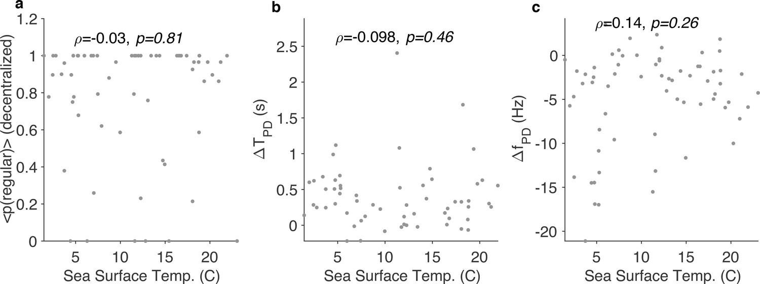
Effects of decentralization do not correlate with seasonal effects.
Probability of observing the regular state during decentralization (a), change in time period of pyloric dilator (PD) neuron (b), and change in firing rate of PD (c) vs. sea surface temperature on the day experiment was carried out. is the Spearman correlation coefficient, and -values are computed using the Spearman rank correlation test.
Figure 8 with 2 supplements
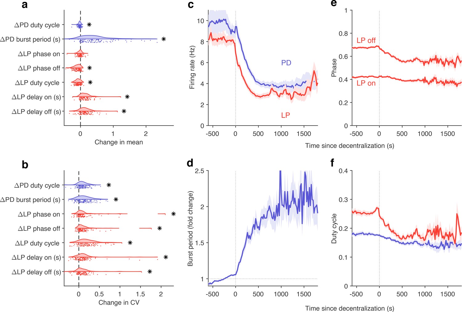
Effects of decentralization on burst metrics.
(a) Change in mean burst metrics on decentralization. (b) Change in coefficient of variation of burst metrics on decentralization. In (a) and (b), each dot is a single preparation; * indicate distributions whose mean is significantly different from zero (p<0.007, paired permutation test). Firing rates (c), burst period (d), lateral pyloric (LP) phases (e), and duty cycles (f) vs. time since decentralization. In (c–f), thick lines indicate population means, and shading indicates the standard error of the mean. points from preparations.
Figure 8—figure supplement 1
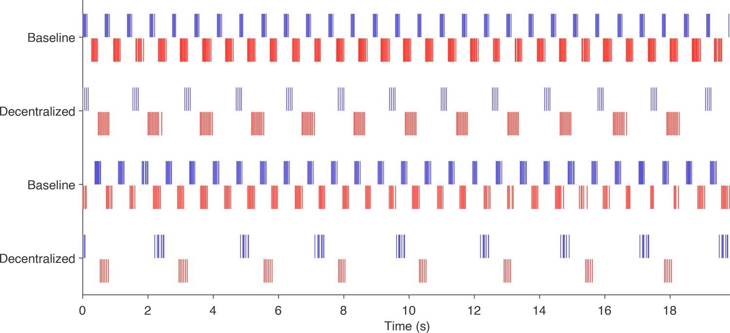
Example rasters showing effect of decentralization.
Rasters from two preparations showing activity before and after decentralization. All of these patterns are classified as regular. Note that the overall rhythm slows down when the preparation is decentralized, but the phase relationships between the bursts are preserved.
Figure 8—figure supplement 2
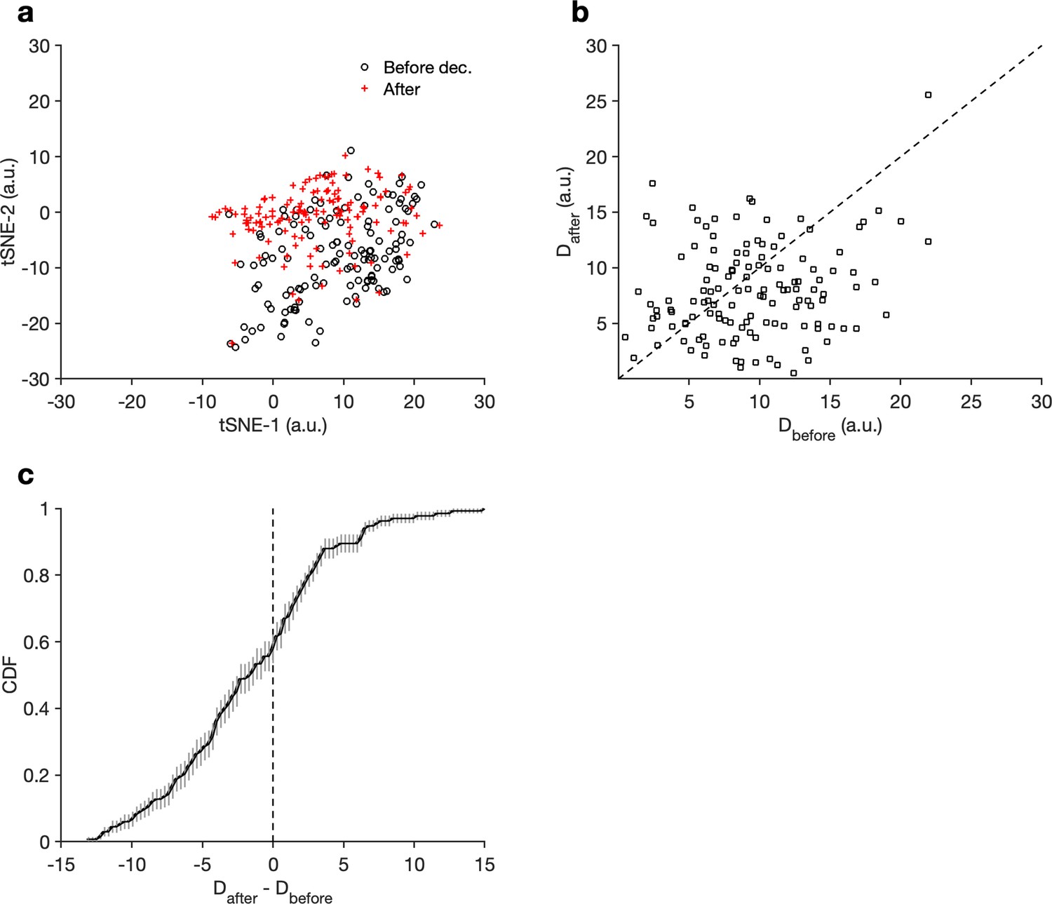
Effects of decentralization on regular rhythms.
(a) Mean locations of data in the regular cluster before and after decentralization. Each preparation is represented by a pair of points, one circle, and one cross. (b) Dispersion (Materials and methods) of data before and after decentralization. Each preparation is a single point. Note that the data appear to be skewed to the right, indicating larger dispersion before decentralization. (c) Distribution of differences in dispersion. The distribution of differences is not significantly skewed from a Gaussian (, Anderson–Darling test), and dispersion in decentralized preparations is significantly lower than in baseline (, paired t-test). points from preparations.
Figure 9 with 2 supplements
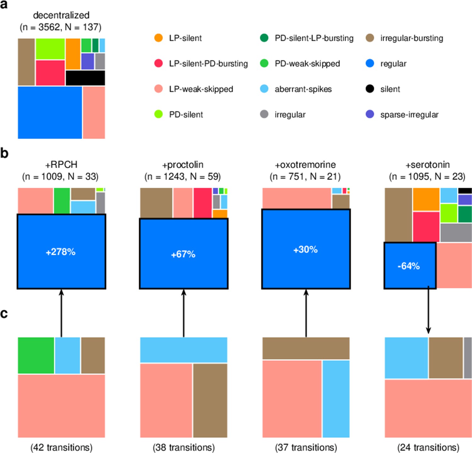
Effect of bath-applied modulators.
(a) State distribution in decentralized preparations. (b) State distribution in bath application of neuromodulators. Change percentages show difference in probability of regular state from decentralized to addition of neuromodulator. (c) Probability distribution of states conditional on transition to (for red pigment-concentrating hormone [RPCH], proctolin, and oxotremorine) or from (for serotonin) the regular state. is the number of data points, and is the number of animals.
Figure 9—figure supplement 1
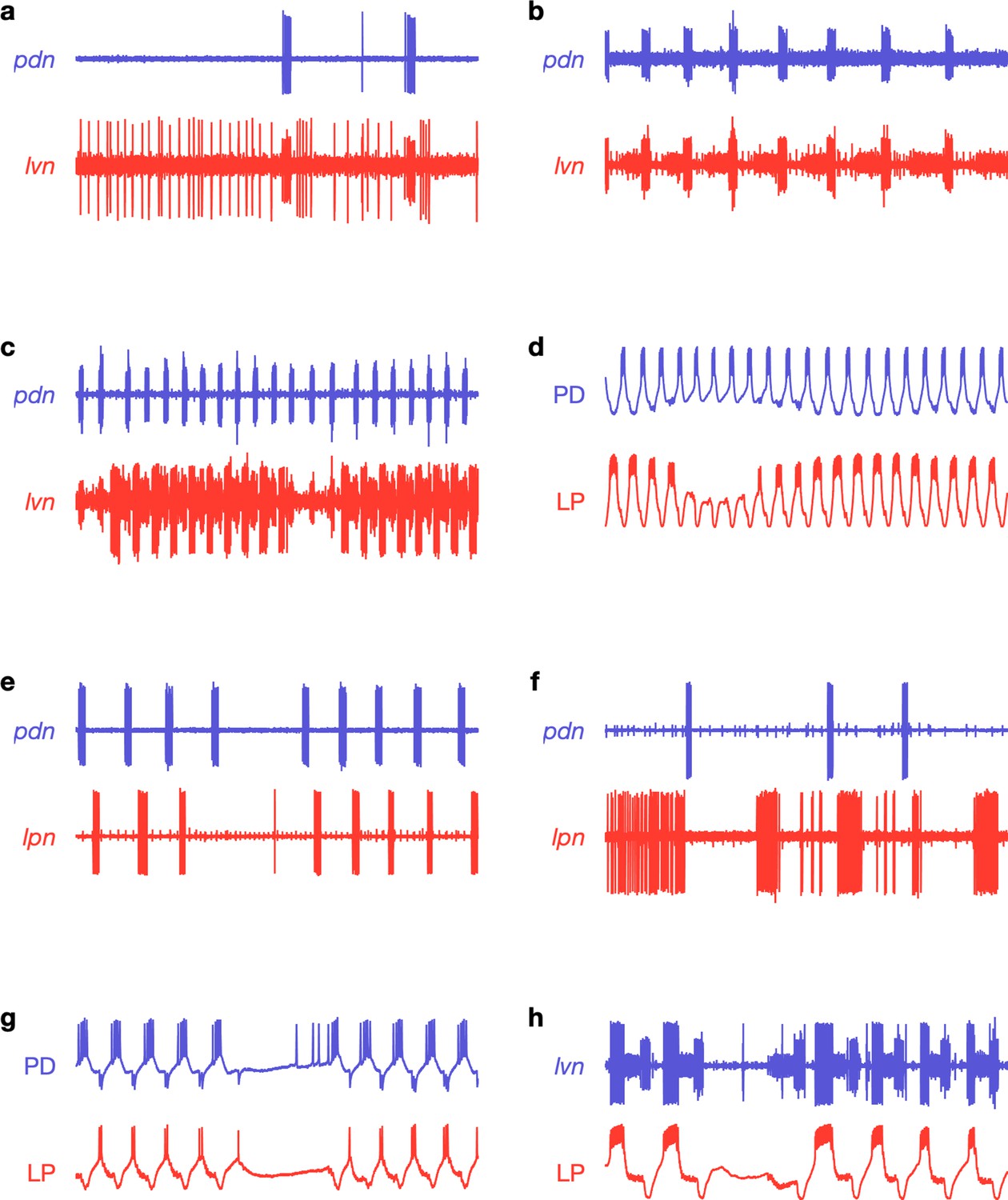
Raw traces during proctolin application.
Nonregular activity patterns in proctolin. Each panel shows a 20 s snippet of raw recordings showing spikes from lateral pyloric (LP; red) and pyloric dilator (PD; blue) neurons. Each panel is from a different animal. Each row is from a different experimenter. (a) Irregular bursting; note prolonged spiking of LP on lvn. (b) LP completely silent; missing from lvn. (c) Intermittent LP interruptions; note breaks in lvn. (d) Interruption in LP bursting. (e) Interruption in PD and LP bursting. (f) Irregular bursting of both PD and LP. (g, h) Interruption of both PD and LP. Traces labeled PD or LP are intracellular recordings.
Figure 9—figure supplement 2
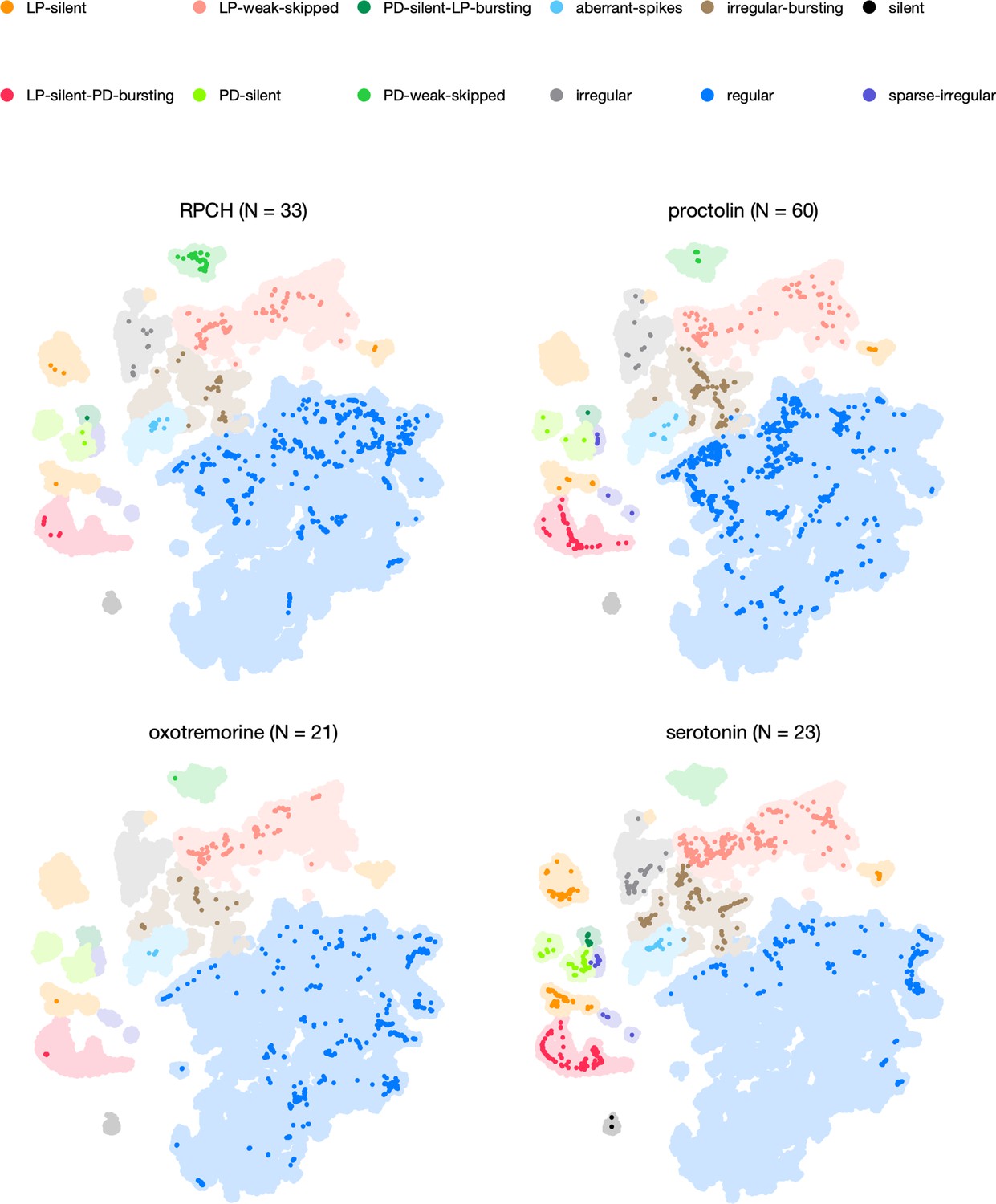
Neuromodulators affect map occupancy.
In each panel, all the data are shown in light shading. Bright colors indicate distribution of data during bath application of that neuromodulator. The number of animals in each panel is indicated in the title.
Figure 10
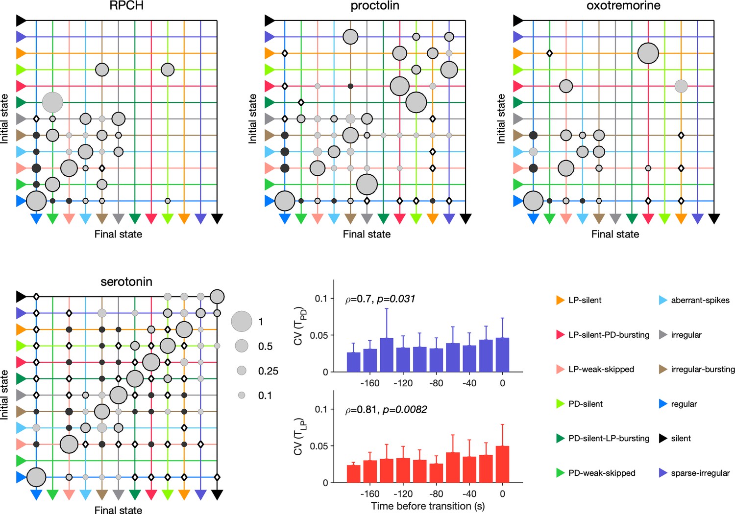
Effect of red pigment-concentrating hormone (RPCH), proctolin, oxotremorine, and serotonin on transition probabilities.
Each matrix shows the conditional probability of observing the final state in the next time step given an observation of the initial state during bath application of that neuromodulator. Probabilities in each row sum to 1. Size of disc scales with probability. Discs with dark borders are transitions that are significantly more likely than the null model (Materials and methods). Dark solid discs are transitions with nonzero probability that are significantly less likely than in the null model. are transitions that are never observed and are significantly less likely than in the null model. States are ordered from regular to silent. Bar graphics show the coefficient of variability (CV) of pyloric dilator (PD) and lateral pyloric (LP) burst periods before transition away from regular states. from Spearman rank correlation test. RPCH: transitions in animals; proctolin: transitions in animals; oxotremorine: transitions in animals; serotonin: transitions in animals. Bar graphs show the CV of burst periods of PD and LP vs. time before a transition away from regular states during serotonin application. from Spearman rank correlation test.
Author response image 1
Tables
Table 1
ANOVA results and power analysis for Figure 4.
ANOVA results for burst metrics in baseline conditions. For each metric, each animal is treated as a group and the variability (mean square difference) is compared within and across group. is the ratio of across-animal to within-animal mean square differences. N.99 is the estimate of the sample size required to reject the null hypothesis with a probability of 0.99 when the alternative hypothesis is true. animals.
| Metric | Across-animal MS | Within-animal MS | F | N.99 |
|---|---|---|---|---|
| LP delay off (s) | 1.1391 | 0.010 956 | 103.97 | 6 |
| LP delay on (s) | 0.616 47 | 0.0111 | 55.54 | 6 |
| LP durations (s) | 0.363 86 | 0.012 366 | 29.424 | 4 |
| LP duty cycle | 0.159 86 | 0.001 309 3 | 122.09 | 10 |
| LP phase off | 0.234 06 | 0.007 227 9 | 32.383 | 11 |
| LP phase on | 0.216 55 | 0.008 811 5 | 24.576 | 9 |
| PD burst period (s) | 3.557 | 0.036 872 | 96.469 | 4 |
| PD durations (s) | 0.079 397 | 0.000 549 44 | 144.5 | 6 |
| PD duty cycle | 0.053 472 | 0.000 413 23 | 129.4 | 16 |
-
LP: lateral pyloric; PD: pyloric dilator.MS: mean square.
Table 2
State counts before and after decentralization for the data shown in Figure 7.
p-Values of change in probability of observing change estimated from paired permutation tests.
| State | ||||
|---|---|---|---|---|
| Regular | 7,967 | 5,791 | lt0.001 | -0.308 77 |
| LP-silent | 22 | 724 | lt0.001 | 0.030 65 |
| LP-silent-PD-bursting | 14 | 577 | lt0.001 | 0.045 926 |
| PD-silent | 11 | 140 | 4 | 0.018 51 |
| PD-silent-LP-bursting | 20 | 18 | 0.469 59 | 0.000 188 91 |
| Aberrant-spikes | 111 | 168 | 0.300 37 | 0.003 285 3 |
| LP-weak-skipped | 317 | 1,628 | lt0.001 | 0.099 875 |
| PD-weak-skipped | 142 | 118 | 0.292 19 | 0.003 453 8 |
| Sparse-irregular | 4 | 154 | lt0.001 | 0.013 263 |
| Irregular | 13 | 116 | 0.000 23 | 0.010 877 |
| Silent | 0 | 321 | lt0.001 | 0.024 825 |
| Irregular-bursting | 72 | 753 | lt0.001 | 0.057 913 |
-
LP: lateral pyloric; PD: pyloric dilator.
Table 3
Probability distribution of states during modulator application, as shown in Figure 9.
| State | Decentralized | RPCH | Proctolin | Oxotremorine | Serotonin |
|---|---|---|---|---|---|
| Regular | 0.39 | 0.73 | 0.69 | 0.78 | 0.27 |
| LP-silent | 0.06 | 0 | 0.02 | 0 | 0.07 |
| LP-silent-PD-bursting | 0.09 | 0 | 0.07 | 0 | 0.1 |
| PD-silent | 0.07 | 0 | 0 | 0 | 0.04 |
| PD-silent-LP-bursting | 0.01 | 0 | 0 | 0 | 0.03 |
| Aberrant-spikes | 0.01 | 0.04 | 0.01 | 0.01 | 0.03 |
| LP-weak-skipped | 0.14 | 0.11 | 0.07 | 0.17 | 0.19 |
| PD-weak-skipped | 0.02 | 0.05 | 0 | 0 | 0 |
| Sparse-irregular | 0.03 | 0 | 0.01 | 0 | 0.02 |
| Irregular | 0.02 | 0.02 | 0.01 | 0 | 0.07 |
| Silent | 0.07 | 0 | 0 | 0 | 0.01 |
| Irregular-bursting | 0.1 | 0.04 | 0.11 | 0.03 | 0.17 |
-
LP: lateral pyloric; PD: pyloric dilator.
Table 4
Code availability.
| Project | Notes |
|---|---|
| sg-s/crabsort | Interactive toolbox to sort spikes from extracellular data |
| sg-s/stg-embedding | Contains all scripts used to generate every figure in this article |
| KlugerLab/FIt-SNE | Fast interpolation-based t-distributed stochastic neighbor embedding, used to make embedding |
| sg-s/SeaSurfaceTemperature | Wrapper to scrape NOAA databases |
Additional files
-
Transparent reporting form
- https://cdn.elifesciences.org/articles/76579/elife-76579-transrepform1-v2.pdf
-
Supplementary file 1
Interactive visualization of pyloric dynamics.
- https://cdn.elifesciences.org/articles/76579/elife-76579-supp1-v2.zip
Download links
A two-part list of links to download the article, or parts of the article, in various formats.
Downloads (link to download the article as PDF)
Open citations (links to open the citations from this article in various online reference manager services)
Cite this article (links to download the citations from this article in formats compatible with various reference manager tools)
Mapping circuit dynamics during function and dysfunction
eLife 11:e76579.
https://doi.org/10.7554/eLife.76579


