Magnetic stimulation allows focal activation of the mouse cochlea
- Department of Neurosurgery, Massachusetts General Hospital, Harvard Medical School, United States
- Department of Otolaryngology - Head and Neck Surgery, Massachusetts Eye and Ear, Harvard Medical School, United States
- Department of Otorhinolaryngology - Head and Neck Surgery, Paracelsus Medical University, Austria
- Program in Speech and Hearing Bioscience and Technology, Harvard Medical School, United States
- Department of Otolaryngology – Head and Neck Surgery, Stanford University School of Medicine, United States
- Boston VA Medical Center, United States
Figures
Figure 1
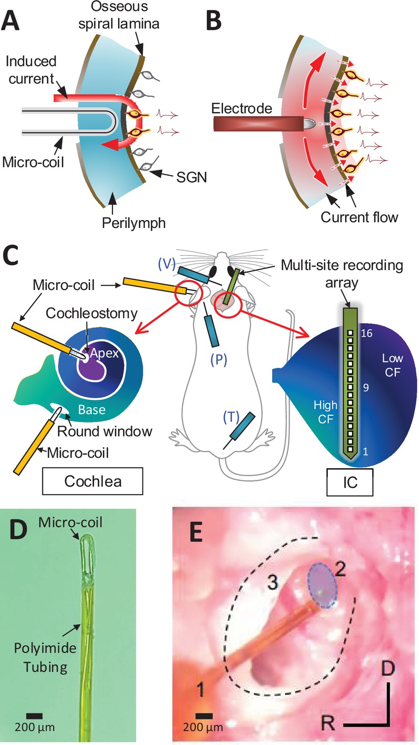
Magnetic stimulation of spiral ganglion neurons (SGNs).
Conceptual diagram illustrating induced electric field generated by a micro-coil (A) and current spread from an electrode (B) positioned in the scala tympani. While high conductivity of the perilymph within the scala tympani leads to an expansive spread of current (B), the induced electric field is confined to tight regions around the coil (A) – see text. (C) Schematic of the experimental setup depicting the micro-coil (orange) inserted into the cochlea (basal and apical turns), the multisite recording array (green) inserted across the tonotopic axis of the inferior colliculus, and placement of three subdermal recording electrodes (blue) into the vertex (V), pinna (P), and tail (T). (D) Photograph of the tip of the micro-coil used in experiments. (E) Photograph of the micro-coil (1) inserted through the round window of the left cochlea into the basal turn (2, shaded blue). The stapedial artery (3) is visible. The outline of the cochlea is approximated by dashed lines. Axes: R: rostral, D: dorsal.
Figure 2 with 2 supplements
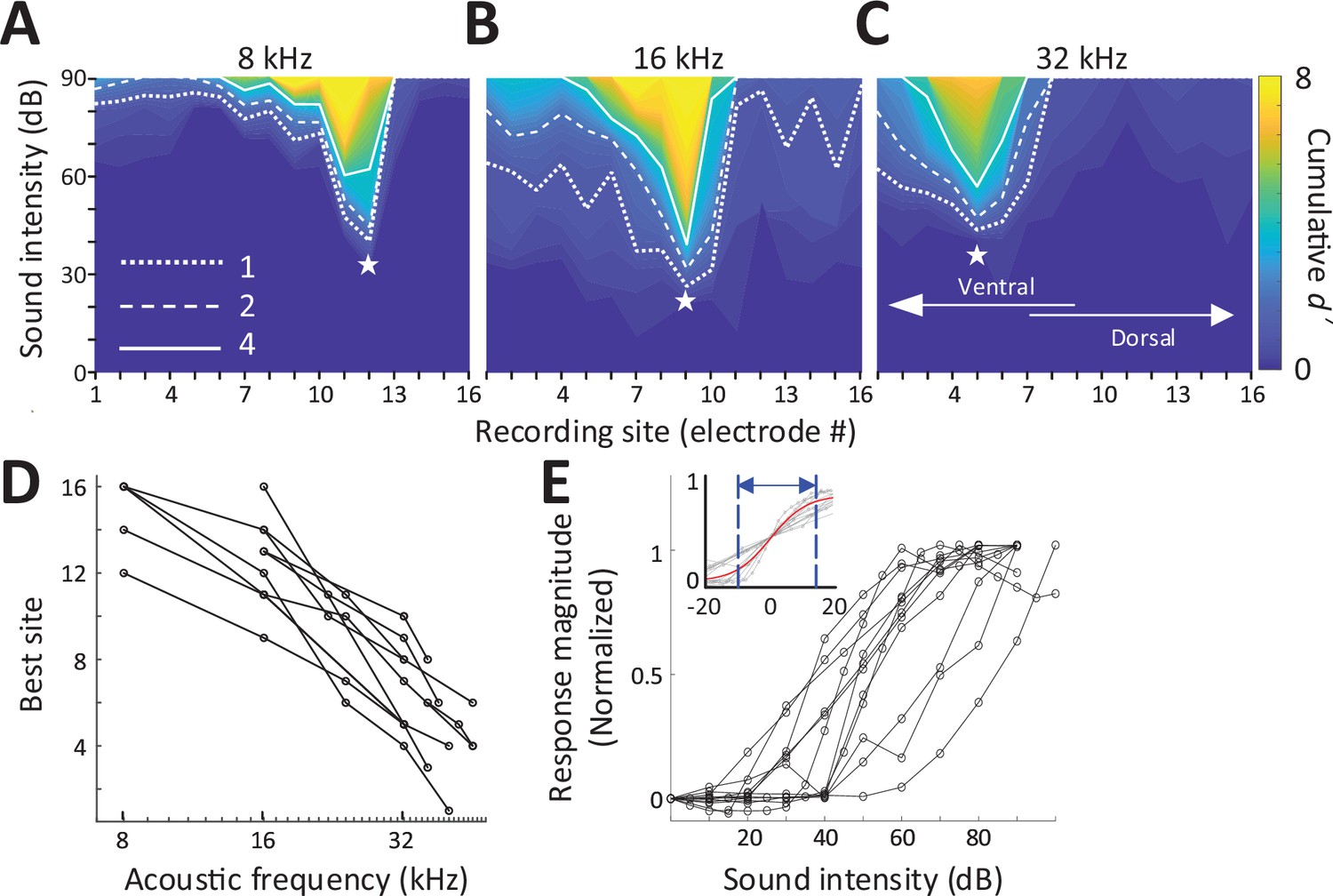
Response to acoustic stimulation measured in the inferior colliculus (IC).
(A–C) Typical spatial tuning curves (STCs) of the IC responses to acoustic stimulation (8, 16, and 32 kHz, respectively) recorded from the 16-channel probe positioned in the IC. Response magnitude was quantified with d-prime analysis (see Materials and methods). The recording site number (x-axis) increases from the IC’s ventral to the dorsal end (low to high characteristic frequency). The recording electrode with the lowest threshold (best site, BS) is marked with a white star. Dotted, dashed and solid lines correspond to cumulative d′ levels of 1, 2, and 4. (D) BS for acoustic stimulation from 8 to 48 kHz; lines connect all data from single animals (n = 11). This mapping is used to assign a ‘characteristic frequency’ to each electrode. (E) Rate-level functions at BS to 32 kHz normalized to peak rate; individual lines are averaged response from individual animals. Inset plots the same data but normalized such that 50% of the amplitude level that elicited the peak response was assigned the level of 0 dB; the solid red line shows the best-fit sigmoidal curve to all data points.
Figure 2—figure supplement 1
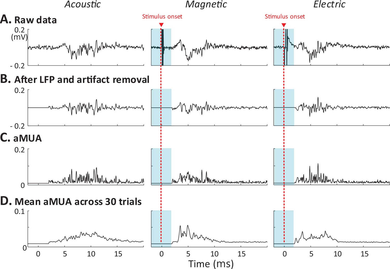
IC responses to acoustic, magnetic, and electric stimulation.
(A) Representative raw recordings of single traces of the neural activity evoked by each stimulation modality were captured by the same recording electrode (positioned in IC). (B) Local field potential was removed from the raw trace by band-pass filtering. The stimulus artifact was removed prior to 2 ms after stimulus onset from the magnetic and electric stimulation responses by setting the response to zero. (C) Analog representation of multiunit activity (aMUA; see Materials and methods). (D) Mean aMUA across 30 trials.
Figure 2—figure supplement 2
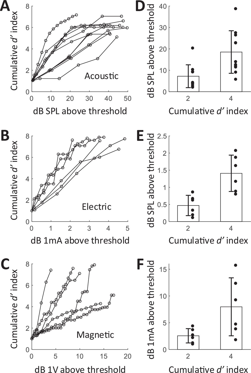
Cumulative d′ index with respect to dB levels above threshold.
The cumulative d′ index at BS plotted as a function of dB above threshold: (A) acoustic stimulation (32 kHz; n = 11 animals), (B) electric stimulation (basal turn; n = 6 animals), and (C) magnetic stimulation (basal turn; n = 6 animals). Individual lines are cumulative d′ index from individual animals. The values of dB above threshold were averaged across animals at d′ = 2 and 4 for acoustic (D), electric (E), and magnetic (F) stimulation. Error bars indicate mean ± standard deviation.
Figure 3 with 1 supplement
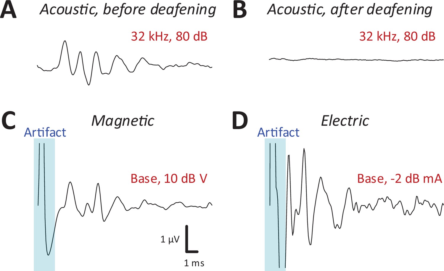
Magnetic stimulation evoked robust auditory brainstem responses (ABRs).
ABR responses to a 32-kHz monotone: (A) control, (B) after DI water was injected into the cochlear through the round window. ABRs from magnetic (C) and electric (D) stimulation (post-deafening). The blue shaded regions identify the portion of the recording obscured by the stimulus artifact.
Figure 3—figure supplement 1
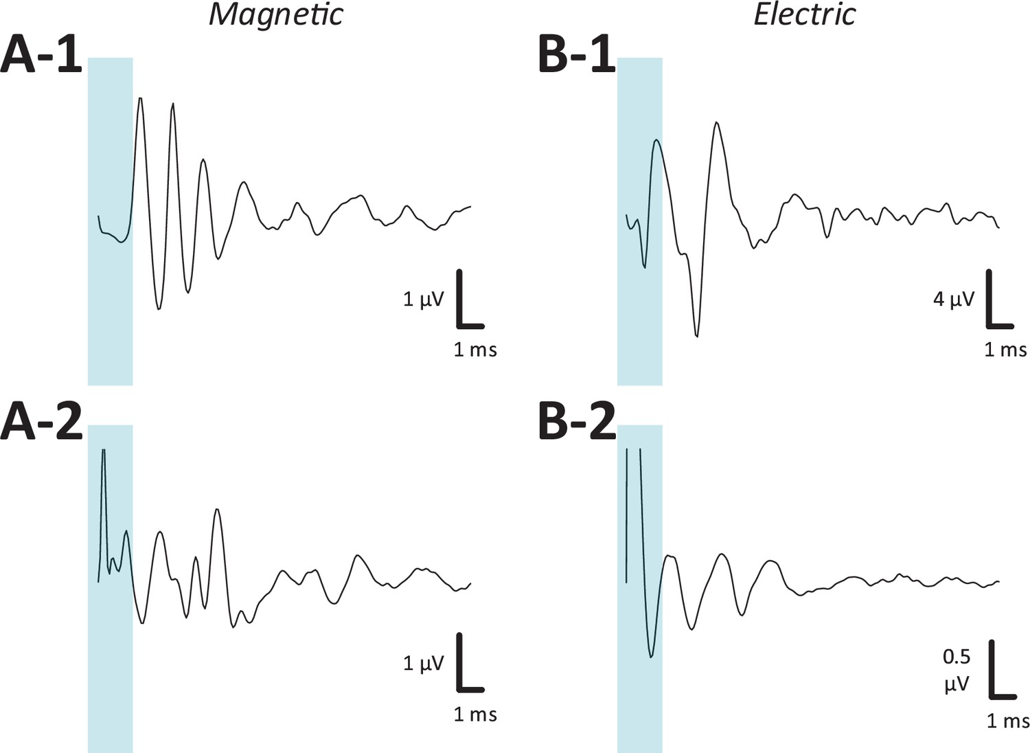
Auditory brainstem responses (ABRs) in response to magnetic and electric stimulation.
(A-1, A-2) ABR responses to magnetic stimulation from two different animals (post-deafening). (B-1, B-2) ABR responses to electric stimulation from two different animals (post-deafening). The blue shaded regions identify the portion of the recording obscured by the stimulus artifact.
Figure 4 with 2 supplements
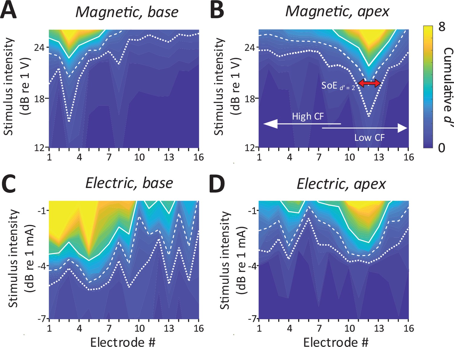
Spatial tuning curves (STCs) for magnetic stimulation are spatially more confined than STCs for electric stimulation.
(A, C) STCs in response to magnetic and electric stimulation delivered to the basal turn of the cochlea (aMUA signals quantified with d-prime analysis – see text). Dotted, dashed, and solid lines are contours for cumulative d′ values of 1, 2, and 4. (B, D) STCs in response to magnetic and electric stimulation of the apical turn. The color bar on the right side of panel B applies to all panels. The red arrow in panel B indicates the spread of excitation (SoE – see text).
Figure 4—figure supplement 1
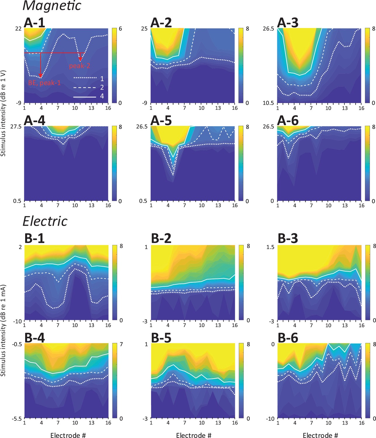
Spatial tuning curves (STCs) in response to magnetic and electric stimulation at the basal turn of the cochlea.
(A-1–A-6) STCs in response to magnetic stimulation delivered to the basal turn of the cochlea from different animals. Dotted, dashed, and solid lines are contours for cumulative d′ values of 1, 2, and 4. Some STCs had more than one peak for both magnetic and electric stimulation. The number of peaks was counted by the number of isolated electrode groups exhibiting a suprathreshold response (d′ > 1) at the stimulus intensity that elicited a cumulative d′ value of 2 as shown in panel A-1. (B-1–B-6) STCs in response to electric stimulation delivered to the basal turn of the cochlea from different animals.
Figure 4—figure supplement 2
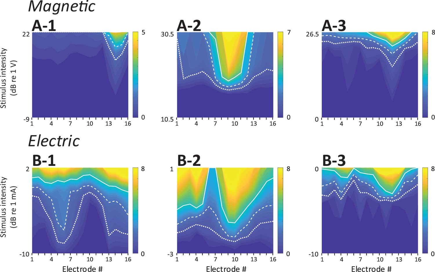
Spatial tuning curves (STCs) in response to apical magnetic and electric stimulation.
(A-1–A-3) STCs in response to magnetic stimulation delivered to the apical turn of the cochlea from different animals. Dotted, dashed, and solid lines are contours for cumulative d′ values of 1, 2, and 4. (B-1–B-3) STCs in response to electric stimulation delivered to the apical turn of the cochlea from different animals.
Figure 5
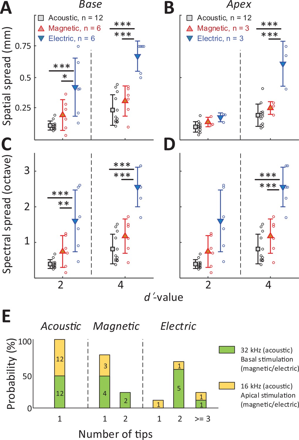
The spread of activation is narrower for magnetic vs. electric stimulation.
(A, B) The spatial spread of IC activation was measured by the width of activated channels at cumulative d′ levels of 2 and 4. (C, D) The spectral spread was estimated by converting the width of activated channels to octave distance based on the characteristic frequency of each electrode (derived from Figure 2D). Two-way ANOVA with subsequent Tukey’s test was applied to verify the statistical significance: *p < 0.05, **p < 0.01, ***p < 0.001. Error bars indicate mean ± standard deviation. (E) The number of tips in the spatial tuning curves (STCs) for each stimulus modality (see text). The numbers inside the bar plots indicate the number of STCs for each group.
Figure 6
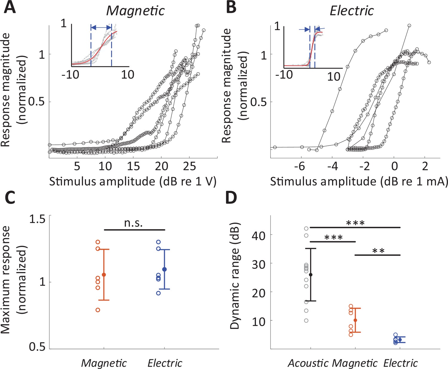
Dynamic range for magnetic stimulation is wider than that for electric stimulation.
Normalized responses rates as a function of stimulus intensity for magnetic (A) and electric (B) stimulation (basal turn). Each line is the averaged response curve from one animal. Insets show the same data normalized such that 50% of the peak response was assigned the level of 0 dB; the red line shows the best-fit curve to all raw data points. (C) Individual points are the distribution of the maximum response rates to magnetic and electric stimulation. Error bars indicate mean ± standard deviation. Each response rate was normalized by the maximum response to acoustic stimulation obtained from the same animal. (D) Individual points are the distribution of dynamic ranges for each mode of stimulation. Error bars indicate mean ± standard deviation. A Student t-test was applied to verify the statistical significance: **p < 0.01, ***p < 0.001.
Figure 7
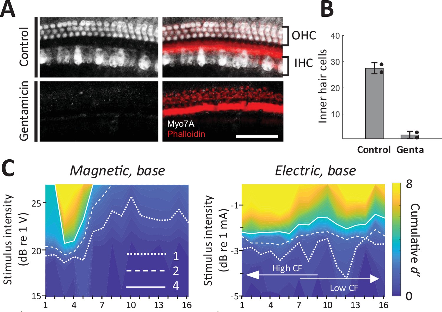
Magnetic stimulation elicits responses in chronically deafened mice.
(A) Gentamicin caused complete loss of inner and outer hair cells (white, Myo7A). Supporting structures of the organ of Corti were stained with Phalloidin (red). Scale bar: 50 µm. (B) Quantification of inner hair cells in the basal turn. Hair cells per 100 µm were counted at 32, 45.25, and 64 kHz. Error bars indicate mean ± standard deviation (n = 2 animals). (C) Spatial tuning curves (STCs) of the IC responses to magnetic and electric stimulation at the base, measured in a gentamicin-treated mouse. Dotted, dashed, and solid lines are contours for cumulative d′ values of 1, 2, and 4, respectively. Data availability: the source data and codes are available on the Open Science Framework (DOI 10.17605/OSF.IO/Y7ZRX).
Tables
Table 1
Statistical analysis of spatial spread (Figure 5A, B) by two-way ANOVA and subsequent Tukey’s test for multiple comparisons; *p < 0.05, ***p < 0.001.
| Predicted (LS) mean diff. | 95.00% CI of diff. | Summary | Adjusted p value | |||
|---|---|---|---|---|---|---|
| Base | d' = 2 | Acoustic vs. magnetic | −0.08433 | −0.2383 to 0.06961 | ns | 0.3863 |
| Acoustic vs. electric | −0.3076 | −0.4615 to −0.1536 | *** | <0.0001 | ||
| Magnetic vs. electric | −0.2233 | −0.4010 to −0.04549 | * | 0.0108 | ||
| d' = 4 | Acoustic vs. magnetic | −0.07223 | −0.2262 to 0.08171 | ns | 0.4953 | |
| Acoustic vs. electric | −0.4324 | −0.5863 to −0.2785 | *** | <0.0001 | ||
| Magnetic vs. electric | −0.3602 | −0.5379 to −0.1824 | *** | <0.0001 | ||
| Apex | d' = 2 | Acoustic vs. magnetic | −0.03936 | −0.1635 to 0.08482 | ns | 0.7172 |
| Acoustic vs. electric | −0.07669 | −0.2009 to 0.04749 | ns | 0.2949 | ||
| Magnetic vs. electric | −0.03733 | −0.1944 to 0.1197 | ns | 0.8287 | ||
| d' = 4 | Acoustic vs. magnetic | −0.05788 | −0.1821 to 0.06630 | ns | 0.4922 | |
| Acoustic vs. electric | −0.4130 | −0.5372 to −0.2889 | *** | <0.0001 | ||
| Magnetic vs. electric | −0.3552 | −0.5122 to −0.1981 | *** | <0.0001 |
Key resources table
| Reagent type (species) or resource | Designation | Source or reference | Identifiers | Additional information |
|---|---|---|---|---|
| Strain, strain background (Mus musculus) | CBA/CaJ | The Jackson Laboratory, Bar Harbor, ME | 000654 | |
| Antibody | Anti-myosin 7A (rabbit polyclonal) | Proteus Biosciences, Ramona, CA | 25-6790 | 1:200 |
| Antibody | Anti-Rabbit IgG (H + L) Cross-Adsorbed Secondary Antibody, Alexa Fluor 488 (goat polyclonal) | Invitrogen, Carlsbad, CA | A-11008 | 1:500 |
| Chemical compound, drug | Gentamicin Sulfate | Sigma-Aldrich, St. Louis, MO | G-4918 | 200 µg |
| Software, algorithm | MATLAB | MathWorks | RRID:SCR_001622 | |
| Software, algorithm | GraphPad Prism | GraphPad | RRID:SCR_ 002798 | |
| Other | Alexa Fluor 647 Phalloidin | Invitrogen, Carlsbad, CA | A22287 | 1:200 |
Additional files
Download links
A two-part list of links to download the article, or parts of the article, in various formats.
Downloads (link to download the article as PDF)
Open citations (links to open the citations from this article in various online reference manager services)
Cite this article (links to download the citations from this article in formats compatible with various reference manager tools)
Magnetic stimulation allows focal activation of the mouse cochlea
eLife 11:e76682.
https://doi.org/10.7554/eLife.76682


