Figures and data in Signal denoising through topographic modularity of neural circuits | eLife

Version of Record

Accepted for publication after peer review and revision.

Download
Cite
Share
CommentOpen annotations (there are currently 0 annotations on this page).

Version of Record published: March 2, 2023 (This version)
Accepted Manuscript published: January 26, 2023 (Go to version)
Accepted: January 25, 2023
Received: January 12, 2022
Preprint posted: January 12, 2022 (Go to version)

Figures
Additional files

10 figures and 6 additional files

Figures

Figure 1 with 1 supplement

Download asset Open asset

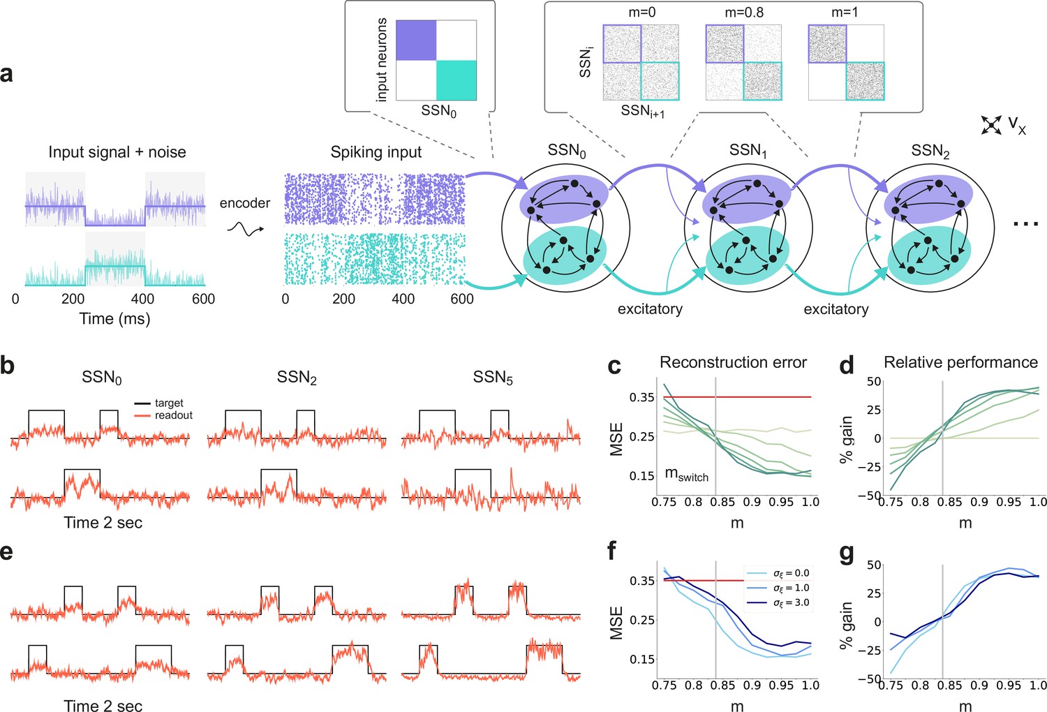
Sequential denoising spiking architecture.

(a) A continuous step signal is used to drive the network. The input is spatially encoded in the first sub-network (SSN₀), whereby each input channel is mapped exclusively onto a sub-population of stimulus-specific excitatory and inhibitory neurons (schematically illustrated by the colors; see also inset, top left). This exclusive encoding is retained to variable degrees across the network, through topographically structured feedforward projections (inset, top right) controlled by the modularity parameter $m$ (see Materials and methods). This is illustrated explicitly for both topographic maps (purple and cyan arrows). Projections between SSNs are purely excitatory and target both excitatory and inhibitory neurons. (b) Signal reconstruction across the network. Single-trial illustration of target signal (black step function) and readout output (red curves) in three different SSNs, for $m = 0.75$ and no added noise ( $σ_{ξ} = 0$ ). For simplicity, only two out of ten input channels are shown. (c) Signal reconstruction error in the different SSNs for the no-noise scenario shown in (b). Color shade denotes network depth, from SSN₀ (lightest) to SSN₅ (darkest). The horizontal red line represents chance level, while the gray vertical line marks the transition (switching) point $m_{switch} \approx 0.83$ (see main text). Figure 1—figure supplement 1 shows the task performance for a broader range of parameters. (d) Performance gain across the network, relative to SSN₀, for the setup illustrated in (b). (e) as in (b) but for $m = 0.9$ . (f) Reconstruction error in SSN₅ for the different noise intensities. Horizontal and vertical dashed lines as in (c). (g) Performance gain in SSN₅, relative to SSN₀.

Figure 1—source data 1 Code and data for Figure 1 and related figure supplements.: https://cdn.elifesciences.org/articles/77009/elife-77009-fig1-data1-v2.zip
Download elife-77009-fig1-data1-v2.zip

Figure 1—figure supplement 1

Download asset Open asset

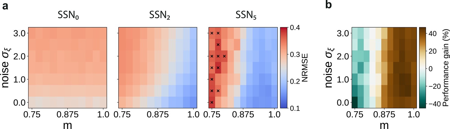
Sequential denoising effect.

(a) Reconstruction error (NRMSE) in three different sub-networks as a function of modularity ( $m$ ) and noise amplitude ( $σ_{ϵ}$ ). The points marked in the rightmost panel correspond to chance-level reconstruction accuracy. (b) Relative reconstruction performance gain in SSN₅ compared to SSN₀, expressed as percentage of error decrease.

Figure 2 with 1 supplement

Download asset Open asset

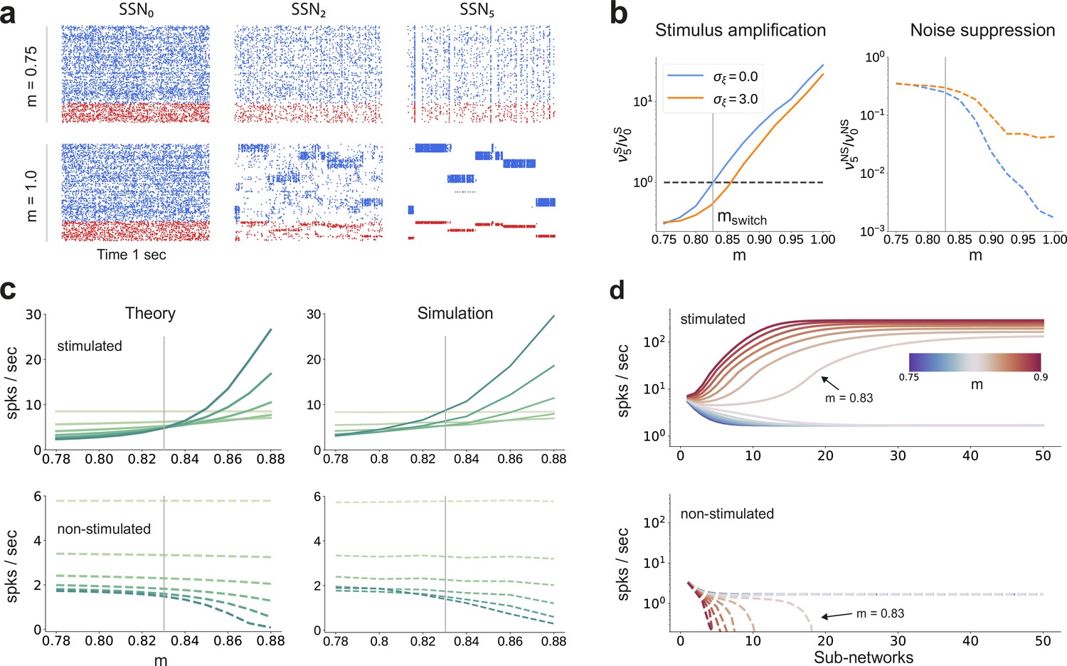
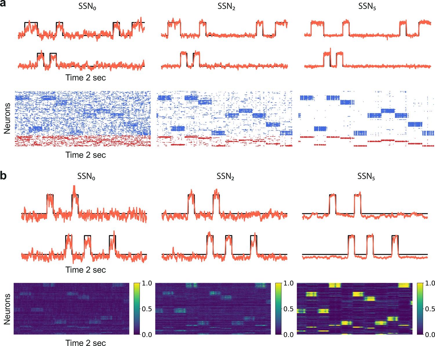
Activity modulation and representational precision.

(a) One second of spiking activity observed across 1000 randomly chosen excitatory (blue) and inhibitory (red) neurons in SSN₀, SSN₂ and SSN₅, for $σ_{ξ} = 3$ and $m = 0.75$ (top) and $m = 1$ (bottom). (b) Mean quotient of firing rates in SSN₅ and SSN₀ $(ν_{5} / ν_{0})$ for stimulated (S, left) and non-stimulated (NS, right) sub-populations for different input noise levels, describing response amplification and noise suppression, respectively. (c) Mean firing rates of the stimulated (top) and non-stimulated (bottom) excitatory sub-populations in the different SSNs (color shade as in Figure 1), for $σ_{ξ} = 0$ . For modularity values facilitating an asynchronous irregular regime across the network, the firing rates predicted by mean-field theory (left) closely match the simulation data (right). (d) Mean-field predictions for the stationary firing rates of the stimulated (top) and non-stimulated (bottom) sub-populations, in a system with 50 sub-networks and $σ_{ξ} = 0$ . Note that all reported simulation data correspond to the mean firing rates acquired over a period of 10 s and averaged across 5 trials per condition. Figure 2—figure supplement 1 shows the firing rates as a function of the input intensity $λ$ .

Figure 2—source data 1 Code and data for Figure 2 and related figure supplements.: https://cdn.elifesciences.org/articles/77009/elife-77009-fig2-data1-v2.zip
Download elife-77009-fig2-data1-v2.zip

Figure 2—figure supplement 1

Download asset Open asset

Mean-field predictions for the gain in the firing rates of stimulated sub-populations.

(a) $ν_{3}^{S} - ν_{2}^{S}$ and (b) $ν_{5}^{S} - ν_{4}^{S}$ , as a function of modularity $m$ and input intensity, scaled by $λ$ (see Materials and methods). Dashed lines demarcate the transition to positive gain.

Figure 3

Download asset Open asset

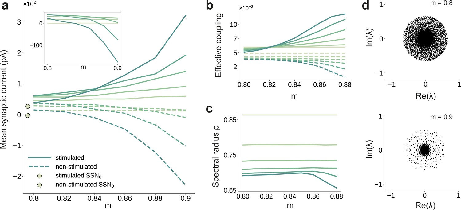
Asymmetric effective couplings modulate the E/I balance and support sequential denoising.

(a) Mean synaptic input currents for neurons in the stimulated (solid curves) and non-stimulated (dashed curves) excitatory sub-populations in the different SSNs. To avoid clutter, data for SSN₀ are only shown by markers (independent of $m$ ). Inset shows the currents (in pA) averaged over all excitatory neurons in the different sub-networks; increasing modularity leads to a dominance of inhibition in the deeper sub-networks. Color shade represents depth, from SSN₁ (light) to SSN₅ (dark). (b) Mean-field approximation of the effective recurrent weights in SSN₅. Curve shade and style as in (a). (c) Spectral radius of the effective connectivity matrices $ρ (W)$ as a function of modularity. (d) Eigenvalue spectra for the effective coupling matrices in SSN₅, for $m = 0.8$ (top) and $m = 0.9$ (bottom). The largest negative eigenvalue (outlier, see Materials and methods), characteristic of inhibition-dominated networks, is omitted for clarity.

Figure 3—source data 1 Code and data for Figure 3.: https://cdn.elifesciences.org/articles/77009/elife-77009-fig3-data1-v2.zip
Download elife-77009-fig3-data1-v2.zip

Figure 4 with 1 supplement

Download asset Open asset

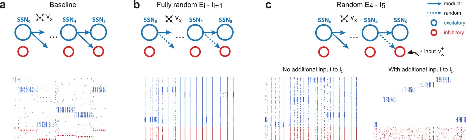
Modular projections to inhibitory populations stabilize network dynamics.

Raster plots show 1 s of spiking activity of 1000 randomly chosen neurons in SSN₅, for different network configurations. (a) Baseline network with $m = 0.88$ . (b) Unstructured feedforward projections to the inhibitory sub-populations lead to highly synchronized network activity, hindering signal representation. (c) Same as the baseline network in (a), but with random projections for $E_{4} \to I_{5}$ and additional but unspecific (Poissonian) excitatory input to $I_{5}$ controlled via $ν_{X}^{+}$ . Without such input ( $ν_{X}^{+} = 0$ , left), the activity is strongly synchronous, but this is compensated for by the additional excitation, reducing synchrony and restoring the denoising property ( $ν_{X}^{+} = 10$ spikes/s, right). Figure 4—figure supplement 1 depicts the activity statistics in the last two modules, for the different scenarios.

Figure 4—source data 1 Code and data for Figure 4 and related figure supplements.: https://cdn.elifesciences.org/articles/77009/elife-77009-fig4-data1-v2.zip
Download elife-77009-fig4-data1-v2.zip

Figure 4—figure supplement 1

Download asset Open asset

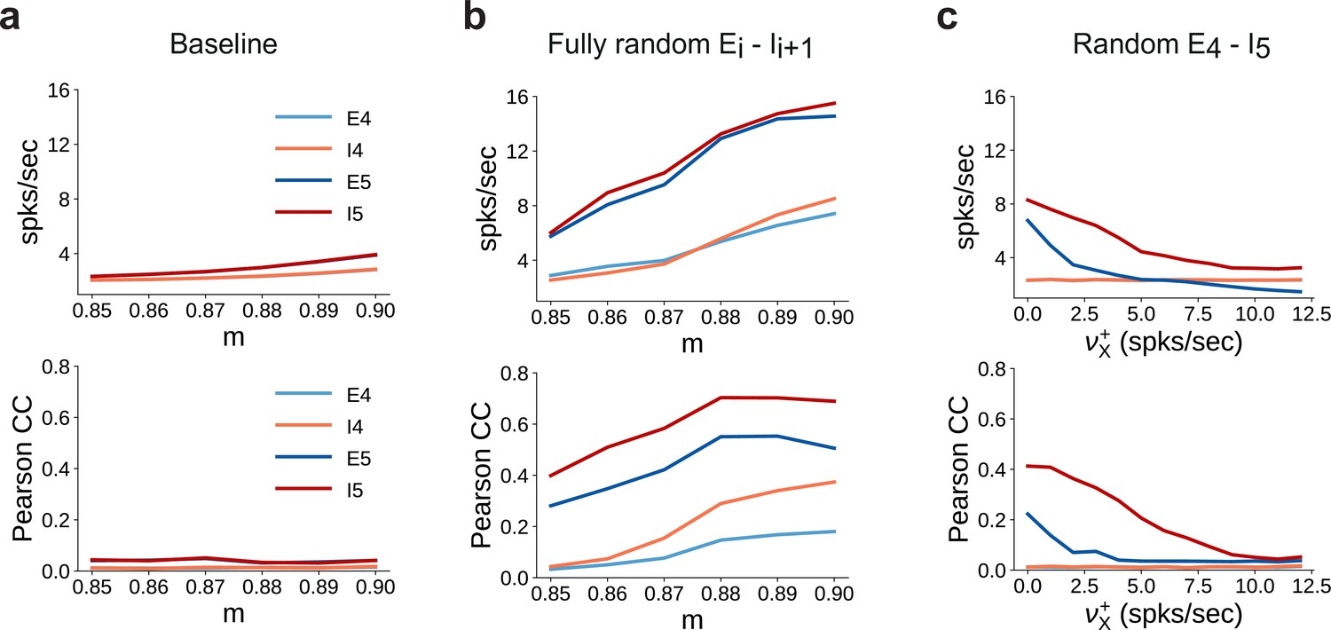
Spiking statistics for different feedforward wiring to inhibitory neurons.

(a) Mean firing rates (top panel) and synchrony (Pearson’s correlation coefficient, computed pairwise over spikes binned into 2 ms bins and averaged across 500 pairs, lower panel) in SSN₄ and SSN₅, as a function of modularity. (b) Same as (a), except with random feedforward projections to the inhibitory pools, that is, $m = 0$ for all $E_{i} \to I_{i + 1}$ connections, $i = {0.4}$ . (c) Same as the baseline network in (a), with $m = 0$ only for $E_{4} \to I_{5}$ . In addition, each neuron in $I_{5}$ receives further excitatory background input with intensity $ν_{X}^{'} = ν_{X} + ν_{X}^{+}$ . Statistics are computed as a function of the additional rate $ν_{X}^{+}$ .

Figure 5 with 1 supplement

Download asset Open asset

Denoising through modular topography is a robust structural effect.

(a) Signal reconstruction (top) and corresponding network activity (bottom) for a network with leaky integrate-and-fire (LIF) neurons and conductance-based synapses (see Materials and methods). Single-trial illustration of target signal (black step function) and readout output (red curves) in three different SSNs, for $m = 0.9$ and strong noise corruption ( $σ_{ξ} = 3$ ). For simplicity, only two out of ten input channels are shown. Figure 5—figure supplement 1 shows additional activity statistics. (b) As in (a) for a rate-based model with $m = 1$ and $σ_{ξ} = 1$ (see Materials and methods for details).

Figure 5—source data 1 Code and data for Figure 5 and related figure supplements.: https://cdn.elifesciences.org/articles/77009/elife-77009-fig5-data1-v2.zip
Download elife-77009-fig5-data1-v2.zip

Figure 5—figure supplement 1

Download asset Open asset

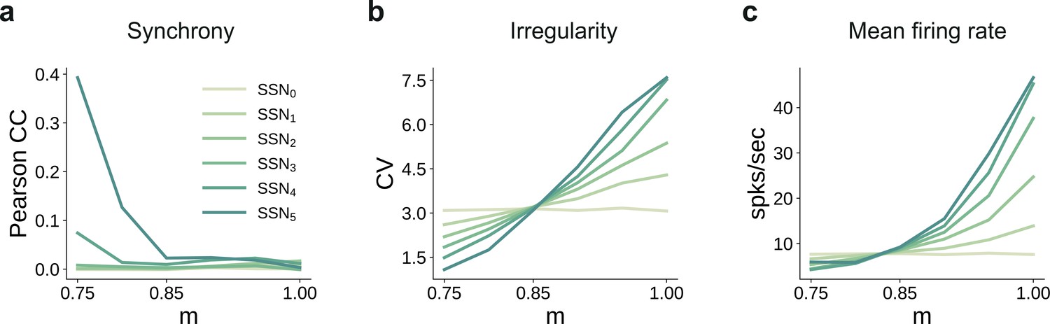
Spiking statistics for the conductance-based model.

(a) Synchrony (Pearson’s correlation coefficient, computed pairwise over spikes binned into 2 ms bins and averaged across 500 pairs); (b) Irregularity measured as the coefficient of variation (CV); (c) Mean firing rate across the excitatory populations. All depicted statistics were averaged over five simulations, each lasting 5 s, with 10 input stimuli.

Figure 6 with 1 supplement

Download asset Open asset

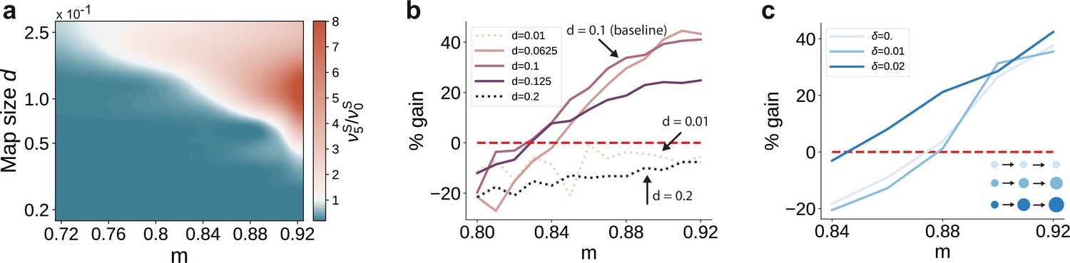
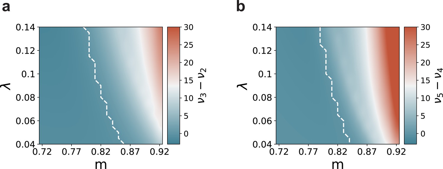
Variation in the map sizes.

(a) Ratio of the firing rates of the stimulated sub-populations in the first and last sub-networks, $ν_{5}^{S} / ν_{0}^{S}$ , as a function of modularity and map size (parameterized by $d$ and constant throughout the network, that is $δ = 0$ , see Materials and methods). Depicted values correspond to stationary firing rates predicted by mean-field theory, smoothed using a Lanczos filter. Note that, in order to ensure that every neuron was uniquely tuned, that is there is no overlap between stimulus-specific sub-populations, the number of sub-populations was igen

chosen to be proportional to the map size ( $N_{C} = 1 / d$ ). (b, c) Performance gain in SSN₅ relative to SSN₀ (ten stimuli, as in Figure 1d, g), for varying properties of structural mappings: (b) fixed map size ( $δ = 0$ ) with color shade denoting map size, and (c) linearly increasing map size ( $δ > 0$ ) and a smaller initial map size $d_{0} = 0.04$ . The results depict the average performance gains measured across five trials, using the current-based model illustrated in Figure 1 (ten stimuli) and no input noise ( $σ_{ξ} = 0$ ). Figure 6—figure supplement 1 further illustrates how the activity varies across the modules as a function of the map size.

Figure 6—source data 1 Code and data for Figure 6 and related figure supplements.: https://cdn.elifesciences.org/articles/77009/elife-77009-fig6-data1-v2.zip
Download elife-77009-fig6-data1-v2.zip

Figure 6—figure supplement 1

Download asset Open asset

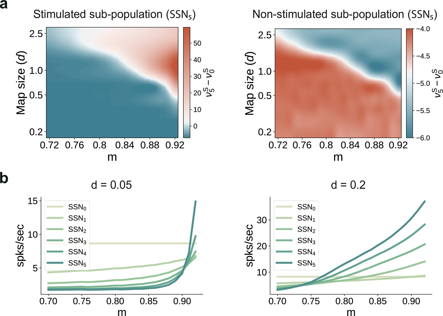
Transition point in modularity decreases with larger map sizes.

(a) Mean-field predictions for the stationary firing rates of the stimulated (left) and non-stimulated sub-populations (right) in SSN₅, as a function of modularity $(m)$ and fixed map size (parametrized by $d$ , see Materials and methods) across the modules $(δ = 0$ ). To limit the impact of additional parameters when varying the map sizes (e.g., overlap), the number of stimulus-specific sub-populations and $d$ where chosen such that every neuron in each population belonged to exactly one stimulus-specific sub-population (see main text for more details). (b) Predicted firing rates in the stimulated sub-populations of the different sub-networks, for $d = 0.05$ (left) and $d = 0.2$ (right), with $δ = 0$ .

Figure 7 with 1 supplement

Download asset Open asset

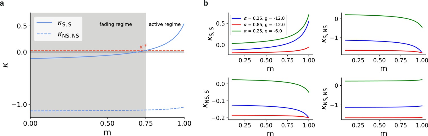
Modularity changes the fixed point structure of the system.

(a) Sketch for self-consistent solution (for the full derivation, see Appendix B) for the firing rate of the stimulated sub-population (blue curves) and the linear relation $κ ν = μ - I$ (orange lines), in the limit of infinitely deep networks. Squares denote stable (black) and unstable (red) fixed points where input and output rates are the same. (b) Bifurcation diagram obtained from numerical evaluation of the mean-field self-consistency equations, Equations 9 and 10 showing a single stable fixed point in the fading regime, and multiple stable (black) and unstable (red) fixed points in the active regime where denoising occurs. (c) Potential energy of the mean activity (see Materials and methods and Equation 22 in Appendix B) for increasing topographic modularity. A stable state, corresponding to local minimum in the potential, exists at a low non-zero rate in every case, including for $m \leq 0.75$ (gray dashed curves, inset). For $m \geq 0.76$ (colored solid curves), a second fixed point appears at progressively larger firing rates. (d) Theoretical predictions for the stationary firing rates of the stimulated and non-stimulated sub-populations in SSN₀, as a function of stimulus intensity ( $λ$ , see Materials and methods). Low, standard, and high denote $λ$ values of 0.01, 0.05 (baseline value used in Figure 1), and 0.25, respectively. (e) Sketch of attractor basins in the potential for different values of $m$ . Markers correspond to the highlighted initial states in (d), with solid and dashed arrows indicating attraction toward the high- and low-activity state, respectively. (f) Firing rates of the stimulated sub-population as a function of modularity in the limit of infinite sub-networks, for the three different $λ$ marked in (d). (g) Modularity threshold for the active regime shifts with increasing noise in the input, modeled as additional input to the non-stimulated sub-populations in SSN₀. Figure 7—figure supplement 1 show the dependency of the effective feedforward couplings on different parameters. Note that all panels (except (a)) show theoretical predictions obtained from numerical evaluation of the mean-field self-consistency equations.

Figure 7—source data 1 Code and data for Figure 7 and related figure supplements.: https://cdn.elifesciences.org/articles/77009/elife-77009-fig7-data1-v2.zip
Download elife-77009-fig7-data1-v2.zip

Figure 7—figure supplement 1

Download asset Open asset

Mean-field predictions for the gain in the firing rates of stimulated sub-populations.

(a) $ν_{3}^{S} - ν_{2}^{S}$ and (b) $ν_{5}^{S} - ν_{4}^{S}$ , as a function of modularity $m$ and input intensity, scaled by $λ$ (see Materials and methods). Dashed lines demarcate the transition to positive gain.

Figure 8 with 2 supplements

Download asset Open asset

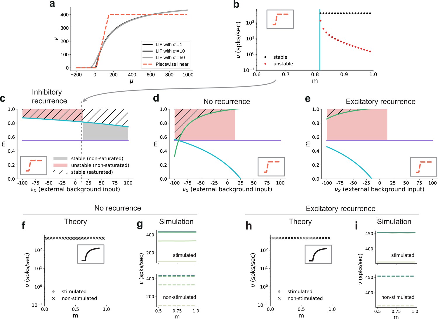
Dependence of critical modularity on neuron and connectivity features.

(a) Activation function $ν (μ, σ)$ for leaky integrate-and-fire model as a function of the mean input μ for $σ = 1, 10, 50$ (black to gray) and piecewise linear approximation with qualitatively similar shape (red). (b) Bifurcation diagram as in Figure 7b, but for piecewise linear activation function shown in inset. Low-activity fixed points at zero rate are not shown, which is the case throughout for the non-stimulated sub-populations. This panel corresponds to the cross-section marked by the gray dashed lines in (c), at $ν_{X} = 12$ . Likewise, the vertical cyan bar corresponds to the lower bound on modularity depicted by the cyan curve in (c) for the same value $ν_{X} = 12$ . (c) Analytically derived bounds on modularity (purple line corresponds to Equation 1, cyan curve to Equation 2) as a function of external input for the baseline model with inhibition-dominated recurrent connectivity ( $g = - 12$ ). Shaded regions denote positions of stable (black) and unstable (red) fixed points with $0 < ν^{S} < ν_{m a x}$ and $ν^{NS} = 0$ . Hatched area represents region with stable fixed points at saturated rates. Denoising occurs in all areas with stable fixed points (hatched and black shaded regions). Negative values on the x-axis correspond to inhibitory external background input with rate $| ν x |$ . (d) Same as panel (c) for networks with no recurrent connectivity within the SSNs (green curve defined by Equation 3). (e) Same as panel (c) for networks with excitation-dominated connectivity within SSNs ( $g = - 3$ ). (f) Same as Figure 7b, obtained through numerical evaluation of the mean-field self-consistent equations for the spiking model. All non-zero fixed points are stable, with points representing stimulated (circle) and non-stimulated (cross) populations overlapping. (g) Mean firing rates across the SSNs in the current-based (baseline) model with no recurrent connections, obtained from 5 s of network simulations and averaged over five trials. (h, i) Same as (f, g) for networks with excitation-dominated connectivity.

Figure 8—source data 1 Code and data for Figure 8 and related figure supplements.: https://cdn.elifesciences.org/articles/77009/elife-77009-fig8-data1-v2.zip
Download elife-77009-fig8-data1-v2.zip

Figure 8—figure supplement 1

Download asset Open asset

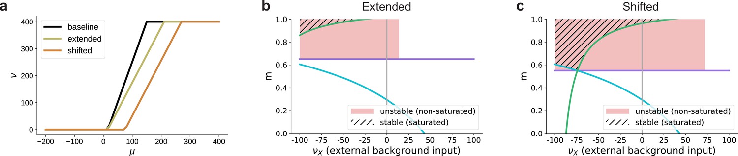
Influence of the activation function’s dynamic range on the bifurcation behavior in excitation-dominated networks ( $g = - 3$ , see also Figure 8e).

(a) The baseline dynamic range $[15, 150]$ is extended to $[15, 210]$ or shifted to $[75, 210]$ . (b) Given that $μ_{\max}$ does not enter the lower bound on the modularity determined by Equation 3 (green curve), extending the dynamic range (see panel (a)) does not affect the region of stable fixed points in the parameter space. For positive background input, there are no stable fixed points, only unstable ones at non-saturated rates for low values of $ν_{X}$ , due to excitatory recurrent fluctuations in the activity. For stronger background input, no fixed points exists where $ν^{S} > ν^{N S}$ . In this case, the activity of the non-stimulated populations (non-zero) dominates the recurrent dynamics and denoising can not be achieved. (c) Shifting the dynamic range altogether (see panel (a)) leads to the emergence of stable fixed points at saturated rates also for positive external input, but the region in which denoising occurs is still significantly smaller than for networks with recurrent inhibition (see Figure 8c). For these values, $ν^{N S} = 0$ is ensured because the total input to the non-stimulated populations remains below the shifted dynamical range, in contrast to just extending the dynamic range where even low inputs can lead to non-zero activity. Moreover, the shifted activation function requires a biologically implausible strength of input for activation. The firing threshold of biological neurons is typically $15 - 20 m V$ above the resting membrane potential, which is much less than the shifted $μ_{\min}$ . Note that similar to Figure 8, here we plot only the fixed points for $ν^{S} > 0$ and $ν^{N S} = 0$ .

Figure 8—figure supplement 2

Download asset Open asset

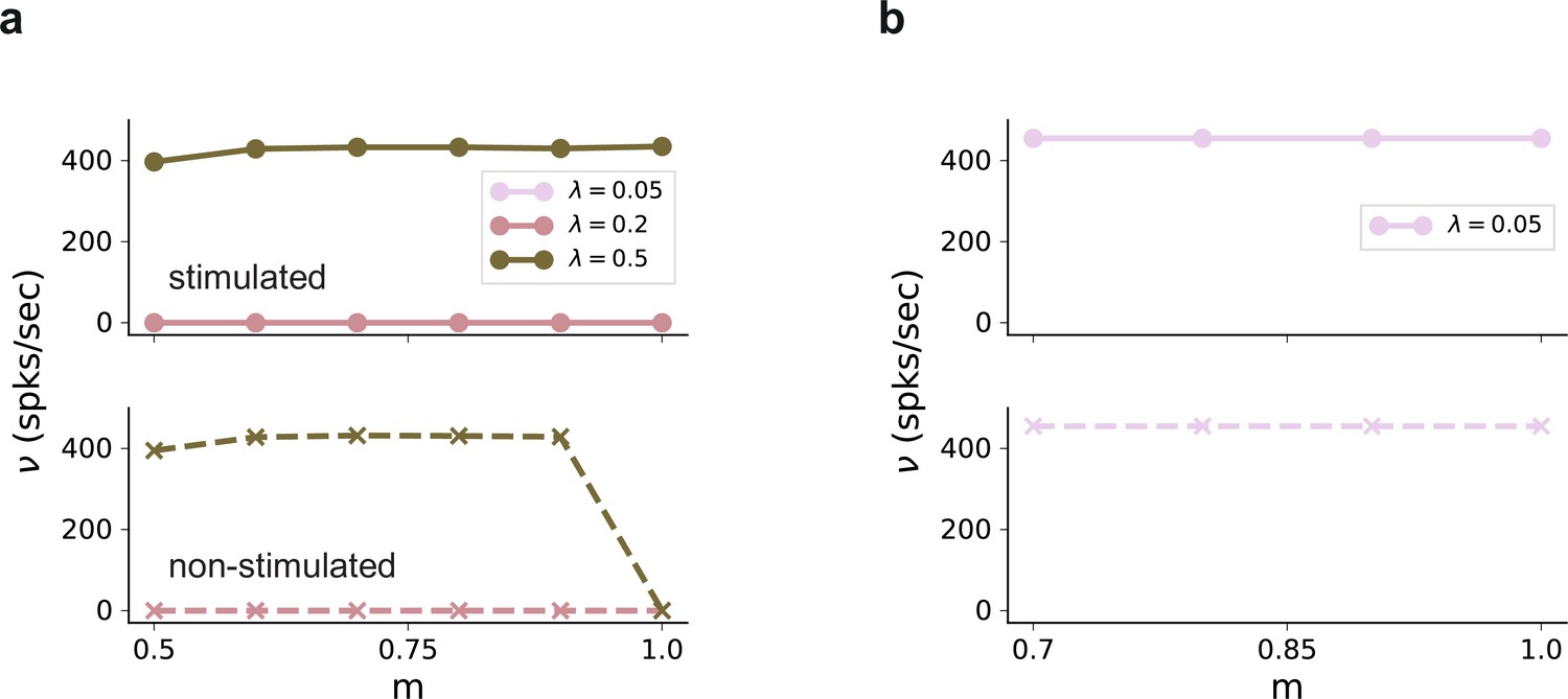
Firing rates in ${SSN}_{5}$ in the absence of external background noise $(ν_{X} = 0)$ .

(a) Firing rates of stimulated (top) and non-stimulated (bottom) populations obtained from simulations of a network without any recurrent connections, for different input intensities $λ$ . Successful denoising only occurs for the extreme case of $m = 1$ , in which case the pathways are completely segregated. Note that the input rate was unchanged, $ν_{in} = 12 λ K_{E}$ . (b) Same as (a), but for excitatory recurrence ( $g = - 3$ ). Recurrent excitation spreads the input from the stimulated pathway to non-stimulated neurons. Results shown only for $λ = 0.05$ , with larger values leading to similar results.

Figure 9 with 2 supplements

Download asset Open asset

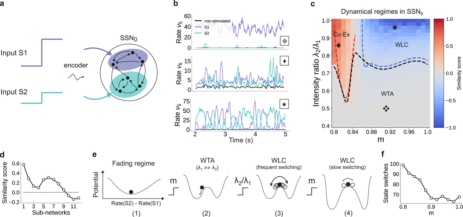
For multiple input streams, topography may elicit a wide range of dynamical regimes.

(a) Two active input channels with corresponding stimulus intensities $λ_{1}$ and $λ_{2}$ , mapped onto non-overlapping sub-populations, drive the network simultaneously. Throughout this section, $λ_{1} = 0.05$ is fixed to the previous baseline value. (b) Mean firing rates of the two stimulated sub-populations (purple and cyan), as well as the non-stimulated sub-populations (black) for three different combinations of $m$ and ratios $λ_{2} / λ_{1}$ (as marked in (c)). (c) Correlation-based similarity score shows three distinct dynamical regimes in SSN₅ when considering the firing rates of two, simultaneously stimulated sub-populations associated with S₁ and S₂, respectively: coexisting (Co-Ex, red area), winner-takes-all (WTA, gray), and winnerless competition (WLC, blue). Curves mark the boundaries between the different regimes (see Materials and methods). Activity for marked parameter combinations shown in (b). (d) Evolution of the similarity score with increasing network depth, for $m = 0.83$ and input ratio of 0.86. For deep networks, the Co-Ex region vanishes and the system converges to either WLC or WTA dynamics. (e) Schematic showing the influence of modularity and input intensity on the system’s potential energy landscape (see Materials and methods): (1) in the fading regime there is a single low-activity fixed point (minimum in the potential); (2) increasing modularity creates two high-activity fixed points associated with S1 and S2, with the dynamics always converging to the same minimum due to $λ_{1} ≫ λ_{2}$ ; (3) strengthening S2 balances the initial conditions, resulting in frequent, fluctuation-driven switching between the two states; (4) for larger $m$ values, switching speed decreases as the wells become deeper and the barrier between the wells wider. (f) Switching frequency between the dominating sub-populations in SSN₅ decays with increasing modularity. Data computed over 10 s, for $λ_{2} / λ_{1} = 0.9$ . Figure 9—figure supplement 1 and Figure 9—figure supplement 2 show the evolution of the Co-Ex region over 12 modules and the potential landscape, respectively.

Figure 9—source data 1 Code and data for Figure 9 and related figure supplements.: https://cdn.elifesciences.org/articles/77009/elife-77009-fig9-data1-v2.zip
Download elife-77009-fig9-data1-v2.zip

Figure 9—figure supplement 1

Download asset Open asset

Evolution of similarity score for 12 sub-networks.

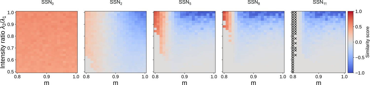
Correlation-based similarity score illustrates the three dynamical regimes observed across the different sub-networks, for two input streams: coexisting (CoEx, red area and positive score), winner-take-all behavior (gray, score near 0), and winnerless competition (WLC, blue and negative score). As predicted by the mean-field analysis, the CoEx region vanishes with increasing network depth. The calculation of the similarity score is detailed in Materials and methods. If either stimuli could not be decoded, we set the score to 0. In SSN₁₁, ‘X’ indicates parameter combinations where none of the stimuli could be decoded.

Figure 9—figure supplement 2

Download asset Open asset

Potential landscape for two input streams.

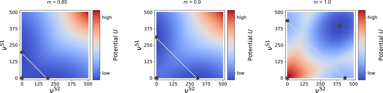
For intermediate modularity ( $m = 0.85$ , left and $m = 0.9$ , right), there are two high-activity fixed points (circled cross markers) in addition to the low-activity one near zero (marker added manually here, as it is not observable due to the larger integration step of 5 spks/sec used here). If the projections are almost fully modular ( $m \approx 1$ ), an additional high-activity fixed point can be observed for identical $ν^{S1}$ and $ν^{S2}$ . In this case, the two stimulated sub-populations can be considered as one larger population, for which the common $κ_{S, S}$ becomes positive, as in the case of a single input stream (see Figure 7—figure supplement 1), just for larger $m$ . Gray, anti-diagonal lines represent the one-dimensional sections illustrated in Figure 9e.

Figure 10 with 1 supplement

Download asset Open asset

Reconstruction of a dynamic, continuous input signal.

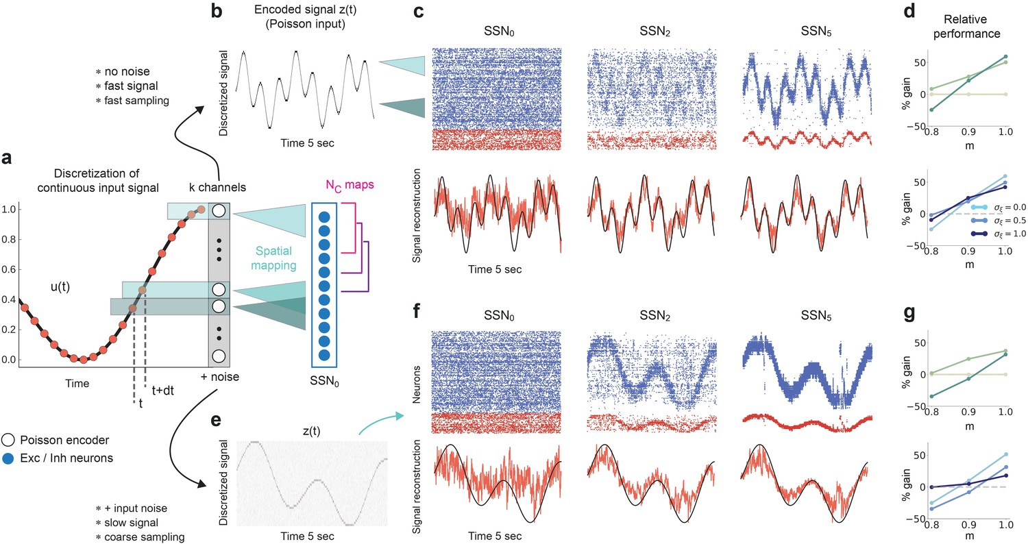
(a) Sketch of the encoding and mapping of a sinusoidal input $x (t)$ onto the current-based network model. The signal is sampled at regular time intervals $d t$ , with each sample binned into one of $k$ channels (which is then active for a duration of $d t$ ). This yields a temporally and spatially discretized $k$ -dimensional binary signal $u (t)$ , from which we obtain the final noisy input $z (t)$ similar to the baseline network (see Figure 1 and Materials and methods). Unlike the one-to-one mapping in Figure 1, here we decouple the number of channels $k = 40$ from that of topographic maps, $N_{C} = 20$ (map size is unchanged, $C_{i} = 800$ ). Because $N_{C} < k$ , the channels project to evenly spaced but overlapping sub-populations in SSN₀, while the maps themselves overlap significantly. (b) Discretized signal $z (t)$ and rate encoding for input $x (t) = \sin (10 t) + \cos (3 t)$ , with $d t = 1 ms$ and no noise ( $σ_{ξ} = 0$ ). (c) Top panel shows the spiking activity of 500 randomly chosen excitatory (blue) and inhibitory (red) neurons in SSN₀, SSN₂, and SSN₅, for $m = 0.9$ . Corresponding target signal $x (t)$ (black) and readout output (red) are shown in bottom panel. (d) Relative gain in performance in SSN₂ and SSN₅ for $σ_{ξ} = 0$ (top). Color shade denotes network depth. Bottom panel shows relative gain in SSN₅ for different levels of noise $σ_{ξ} \in {0, 0.5, 1}$ . (e–g) Same as (b–d), but for a slowly varying signal (sampled at $d t = 20 ms$ ), $σ_{ξ} = 0.5$ and $m = 1$ . Performance results are averaged across five trials. We used 20 s of data for training and 10 s for testing (activity sampled every 1 ms, irrespective of input discretization $d t$ ).

Figure 10—source data 1 Code and data for Figure 10 and related figure supplements.: https://cdn.elifesciences.org/articles/77009/elife-77009-fig10-data1-v2.zip
Download elife-77009-fig10-data1-v2.zip

Figure 10—figure supplement 1

Download asset Open asset

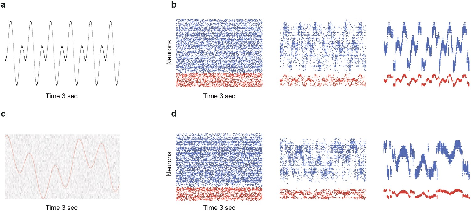
Limits of denoising for rapidly changing and noisy dynamical inputs.

(a) A fast changing input signal $x (t) = \sin (24 t) + \cos (12 t)$ sampled at $d t = 1 m s$ , with no additional noise ( $σ_{ξ} = 0$ ). (b) While portions of the signal can be successfully transmitted and denoised in SSN₅, there are significant periods (steep slopes) where the signal representation is lost. (c) Slower signal $x (t) = \sin (10 t) + \cos (3 t)$ with significant noise corruption ( $σ_{ξ} = 2 ν_{in}$ ). Continuous red curve denotes the input signal $u (t)$ . (d) Strong noise in the input leads to heavy fluctuations in the activity of the deeper populations, corrupting the signal representations.

Additional files

Supplementary file 1 Tabular description of current-based (baseline) network model.: https://cdn.elifesciences.org/articles/77009/elife-77009-supp1-v2.pdf
Download elife-77009-supp1-v2.pdf
Supplementary file 2 Model parameters for the current-based network.: https://cdn.elifesciences.org/articles/77009/elife-77009-supp2-v2.pdf
Download elife-77009-supp2-v2.pdf
Supplementary file 3 Parameter values for the conductance-based model.: https://cdn.elifesciences.org/articles/77009/elife-77009-supp3-v2.pdf
Download elife-77009-supp3-v2.pdf
Supplementary file 4 Description of the rate model.: https://cdn.elifesciences.org/articles/77009/elife-77009-supp4-v2.pdf
Download elife-77009-supp4-v2.pdf
Supplementary file 5 Rate model parameters.: https://cdn.elifesciences.org/articles/77009/elife-77009-supp5-v2.pdf
Download elife-77009-supp5-v2.pdf
Transparent reporting form: https://cdn.elifesciences.org/articles/77009/elife-77009-transrepform1-v2.pdf
Download elife-77009-transrepform1-v2.pdf

Download links

A two-part list of links to download the article, or parts of the article, in various formats.

Downloads (link to download the article as PDF)

Open citations (links to open the citations from this article in various online reference manager services)

Mendeley

Cite this article (links to download the citations from this article in formats compatible with various reference manager tools)

Barna Zajzon
David Dahmen
Abigail Morrison
Renato Duarte

(2023)

Signal denoising through topographic modularity of neural circuits

eLife 12:e77009.

https://doi.org/10.7554/eLife.77009

Sign up for email alerts

Privacy notice