Vocal communication is tied to interpersonal arousal coupling in caregiver-infant dyads
- Department of Psychology, University of East London, United Kingdom
- Institute of Psychiatry, Psychology & Neuroscience, King's College London, United Kingdom
- Université Grenoble Alpes, France
Figures
Figure 1
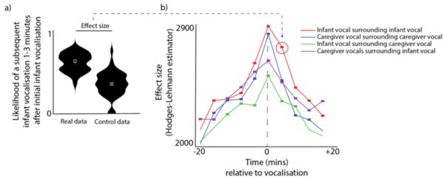
Vocalisation clusters.
(a) Sample violin plot showing the analysis for one time interval that was then repeated iteratively across multiple time intervals in b. The plot shows the likelihood of a subsequent infant vocalisation in the time window 1–3 min following an infant vocalisation, comparing real with control data. (b) Same analysis repeated across multiple time windows, and across different categories. Coloured rectangles indicate time bins in which real >control after correction for multiple comparisons using a permutation-based temporal clustering procedure. Y-axis shows the Hodges-Lehman effect size of the Mann Whitney test comparing observed and control data.
Figure 2

arousal changes around vocalisations.
(a) Histogram showing the distribution of arousal levels at the time of each vocalisation. (b) Change in arousal levels during the period from 20 min before to 20 min after each vocalisation. Shaded areas show standard error, based on an N of 82. Coloured rectangles indicate areas in which observed >0 after correcting for multiple comparisons using a permutation-based temporal clustering procedure. (c) Sample violin plot showing analysis for one time interval that was then repeated iteratively across multiple time intervals in e. The plot shows the likelihood of a subsequent infant vocalisation in the time window 1–3 min following a peak in infants’ arousal (10% highest values), comparing real with control data. (d) Receiver Operating Characteristic (ROC) Area Under the Curve (AUC) results. 0.5 shows a chance result. Error bars show the between-participant standard error of the means, based on an N of 82. * indicates significant difference from chance p<0.05, using the Mann-Whitney U test. (e) Same analysis as illustrated in c, repeated across multiple time windows, and across different categories. Y-axis shows the effect size of the Mann Whitney test comparing observed and control data. Coloured rectangles indicate time bins in which real >control after correction for multiple comparisons using a permutation-based temporal clustering procedure.
Figure 3
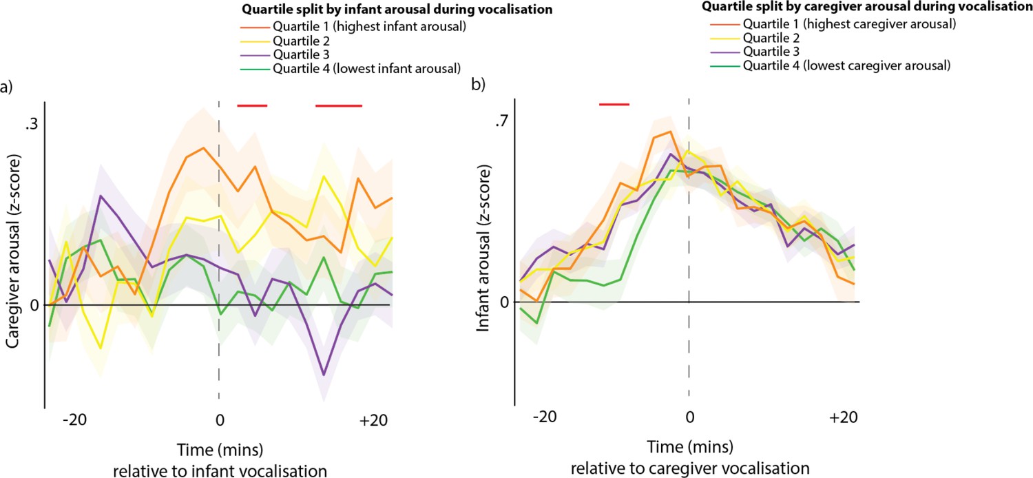
Arousal changes across the dyad following vocalisations.
(a) Caregiver arousal subdivided by infant arousal at the time of the vocalisation. (b) Infant arousal subdivided by caregiver arousal at the time of the vocalisation. For all plots, shaded areas indicate standard error based on an N of 82, and red highlights indicate areas of significant difference after correction for multiple comparisons using a permutation-based temporal clustering procedure.
Figure 4

Arousal stability and coupling around vocalisations.
(a) Infant arousal stability relative to caregiver vocalisations; (b) infant arousal stability relative to infant vocalisations; (c) infant arousal stability relative to infant cries; (d) infant arousal stability relative to infant speech-like vocalisations; (e) caregiver arousal stability relative to caregiver vocalisations; (f) caregiver arousal stability relative to infant vocalisations; (g) caregiver arousal stability relative to infant cries; (h) caregiver arousal stability relative to infant speech-like vocalisations; (i) infant-caregiver arousal coupling relative to caregiver vocalisations; (j) infant-caregiver arousal coupling relative to infant vocalisations; (k) infant-caregiver arousal coupling relative to infant cries; (l) infant-caregiver arousal coupling relative to infant speech-like vocalisations. Black shows the real data; grey shows the control data. Error bars show the standard errors based on an N of 82 for a-h and 74 for i-l. Sections highlighted in red indicate areas of significant difference between real and control data after correction for multiple comparisons using a permutation-based temporal clustering procedure.
Figure 5

Vocalisation clusters and arousal around vocalisations subdivided by infant vocalisation type.
(a) Likelihood of infant and caregiver vocalisations during the time period before and after known infant vocalisations. (b) Likelihood of infant cries and speech-like vocalisations during the time period relative to infant 90th centile arousal peaks. (c) Change in arousal levels relative to vocalisations. Shaded areas show the standard errors based on an N of 82. For all plots, coloured rectangles indicate time windows in which real >control after correction for multiple comparisons using a permutation-based temporal clustering procedure. (d) Plot showing same data as 5 c, but showing pre- vs post-vocalisation differences in arousal around cries and speech-like vocalisations. Values above 0 indicate that post vocalisation arousal >pre vocalisation arousal. (e) Receiver Operating Characteristic (ROC) Area Under the Curve (AUC) results. 0.5 shows a chance result. Error bars show the between-participant standard error of the means based on an N of 82. * indicates significant difference from chance p<0.05, * indicates significant difference from chance p<0.05, using the Mann-Whitney U test.
Figure 6
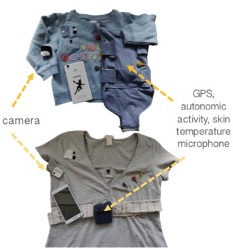
Photographs of recording equipment used.
Figure 7
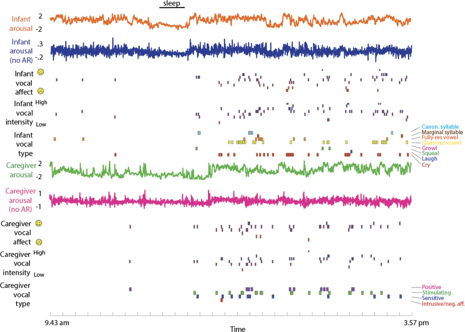
Raw Data Sample.
from top to bottom: infant arousal composite score (see SM sections 1.2–1.5); infant arousal after removal of the auto-correlation (see SM section 1.6); infant vocal affect (see Methods section); infant vocal intensity; infant vocalisation type; caregiver arousal; caregiver arousal after removal of the auto-correlation; caregiver vocal affect; caregiver vocal intensity; caregiver vocalisation type.
Figure 8
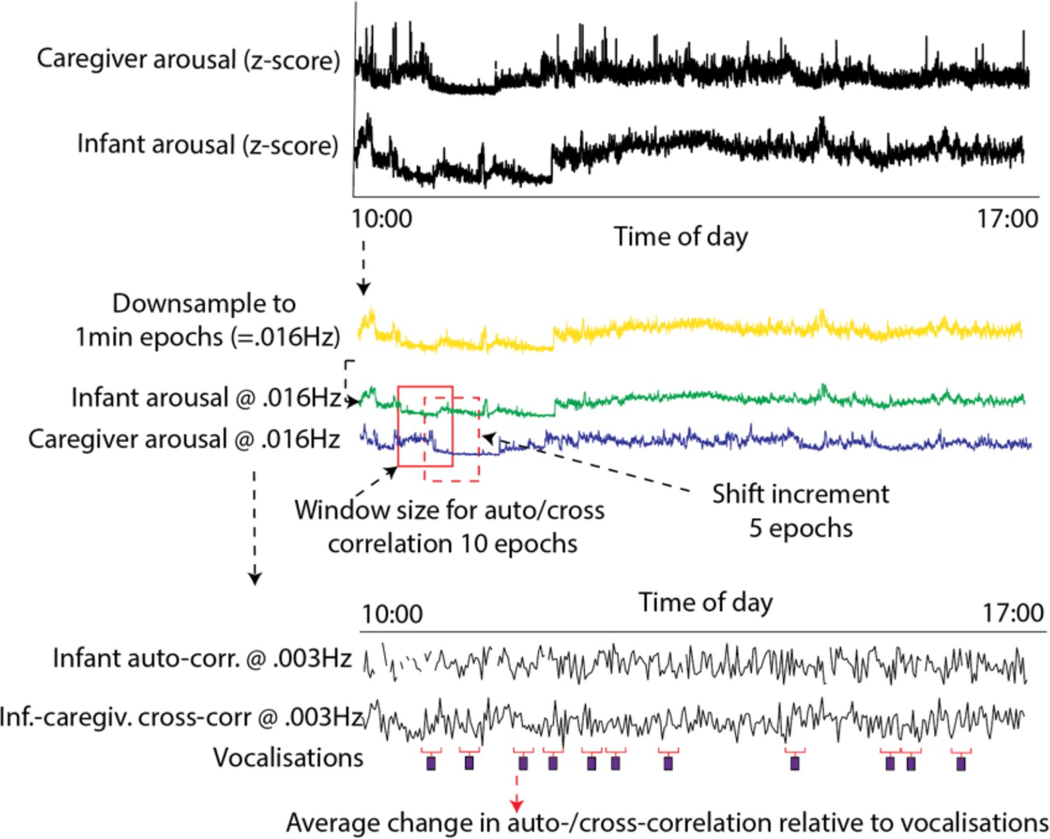
Schematic illustrating the auto- and cross-correlation analyses.
Arousal data were downsampled to 1 min epochs (corresponding to the sampling frequency of the microphone data). The windowed auto- and cross-correlation was then calculated, using a window size of 10 epochs, which shifted 5 epochs between windows. The average change in auto- and cross-correlation relative to vocalisations was then calculated.
Appendix 1—figure 1
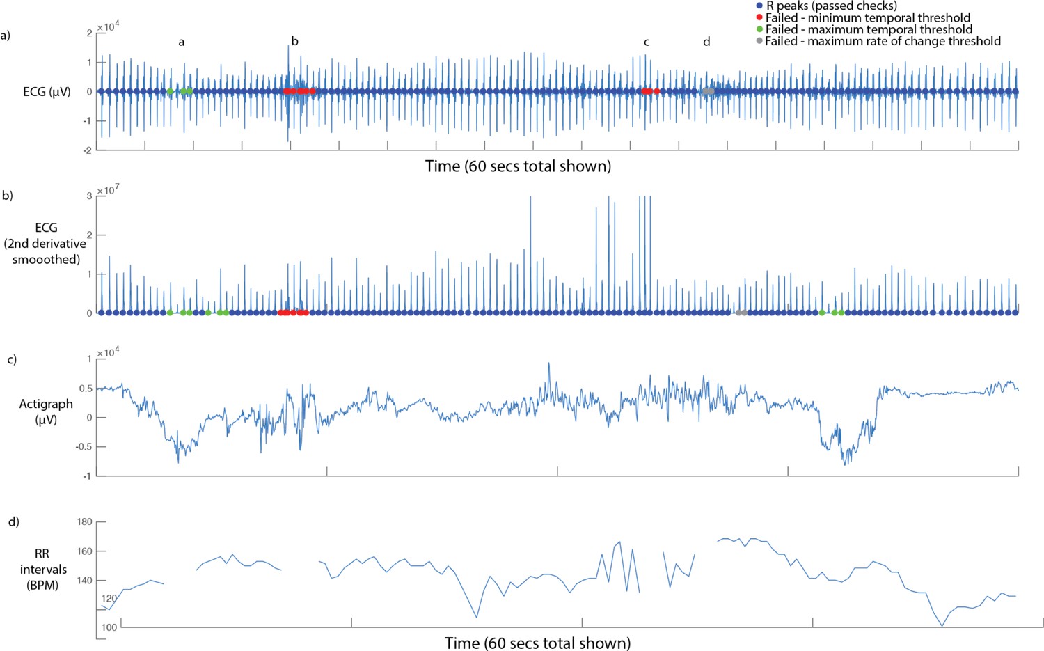
Sample screenshot from ECG parsing algorithm.
60 seconds’ data is shown. From top to bottom: (i) raw ECG signal. Coloured dots show the results of the three checks described in the main text, below (see legend); (ii) smoothed second derivative of ECG signal. This measure was not used as our pilot analyses found it to be less effective than applying the processing to the raw signal; (iii) raw (unprocessed) actigraph data. This information was only used for visual inspection, and was not used in parsing; (iv) RR intervals (in BPM), with rejected data segments excluded.
Appendix 1—figure 2
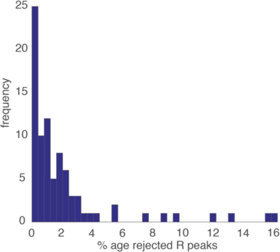
Histogram showing the proportion of rejected R peaks (as identified using the three criteria described above).
Appendix 1—figure 3
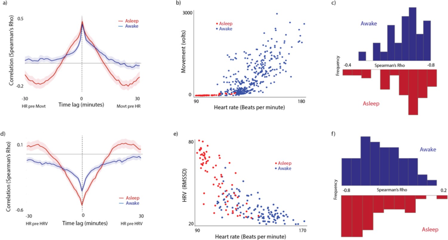
Illustrating the relationship between the individual physiological measures included in the composite measure.
(a) Cross-correlation of the relationship between HR and Movement. (b) Scatterplot from a sample participant. Each datapoint represents an individual 60-s epoch of data. (c) Histograms showing the average zero-lagged correlation between 60-s epochs, calculated on a per-participant basis and then averaged. (d-f) Equivalent plots for Heart rate and Heart rate variability.
Appendix 1—figure 4
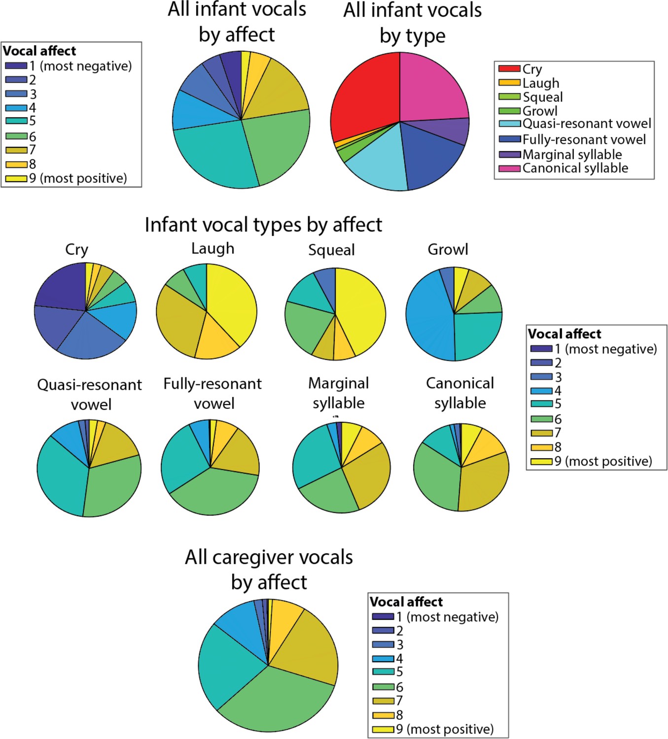
Pie charts showing infant vocalisation type by vocal affect.
Appendix 1—figure 5
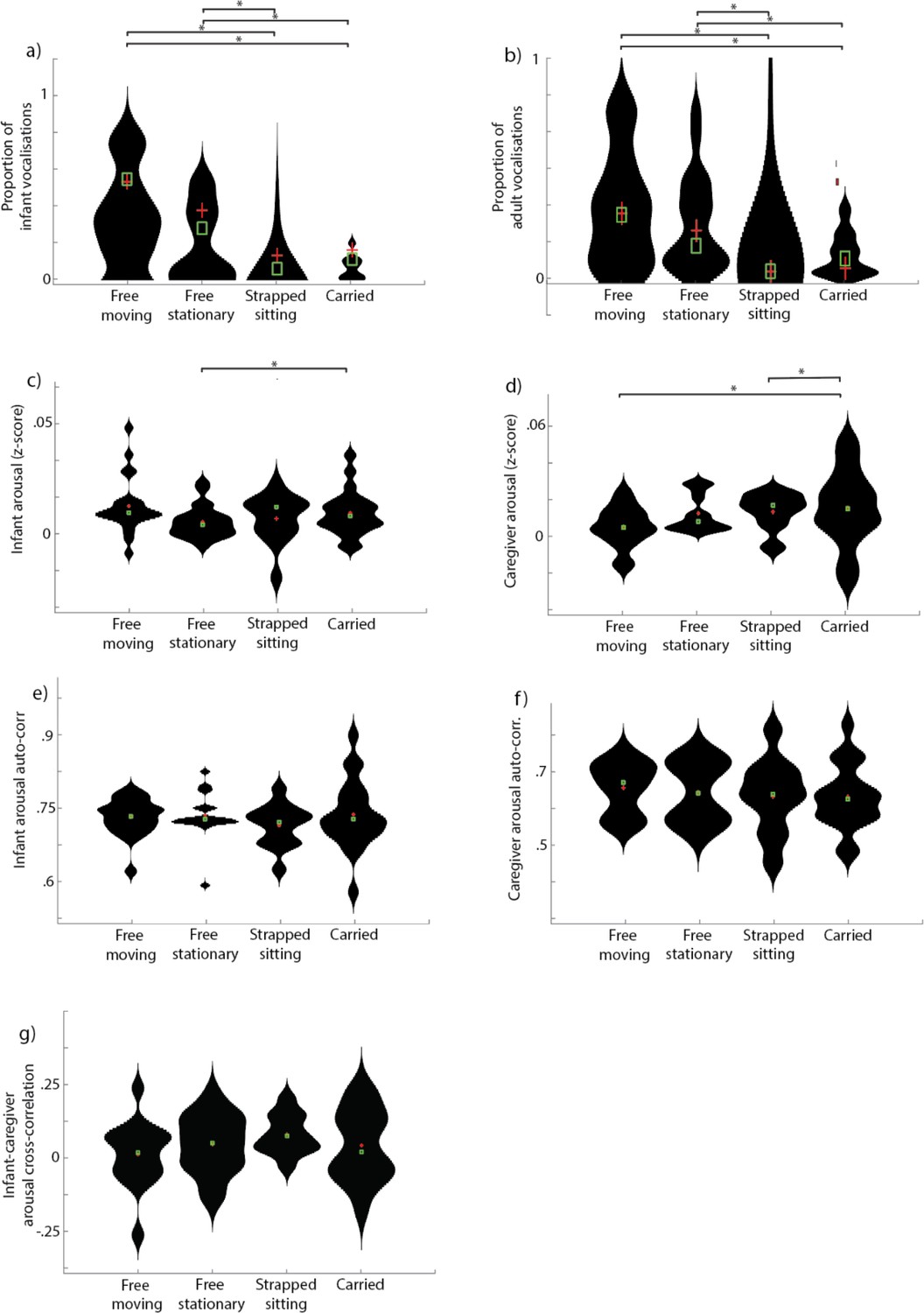
Violin plots showing results of physical position coding.
(a) and (b) show proportion of infant vocalisations and proportion of adult vocalisations in each of the four physical positions coded. (c) and (d) show infant arousal in each of the four physical positions coded. (e) and (f) show arousal auto-correlation in each of the four physical positions coded. (g) shows infant-caregiver arousal cross-correlation in each of the four physical positions coded. For all analyses, * indicates significant pairwise post hoc between group comparison after correcting for multiple comparisons, p<0.05.
Appendix 1—figure 6

Arousal changes around vocalisations based on micro-level coding.
(a) Same as Figure 2b in the main text, examining infant and caregiver arousal changes to infant and caregiver vocalisations. Shaded areas show standard errors.
Appendix 1—figure 7
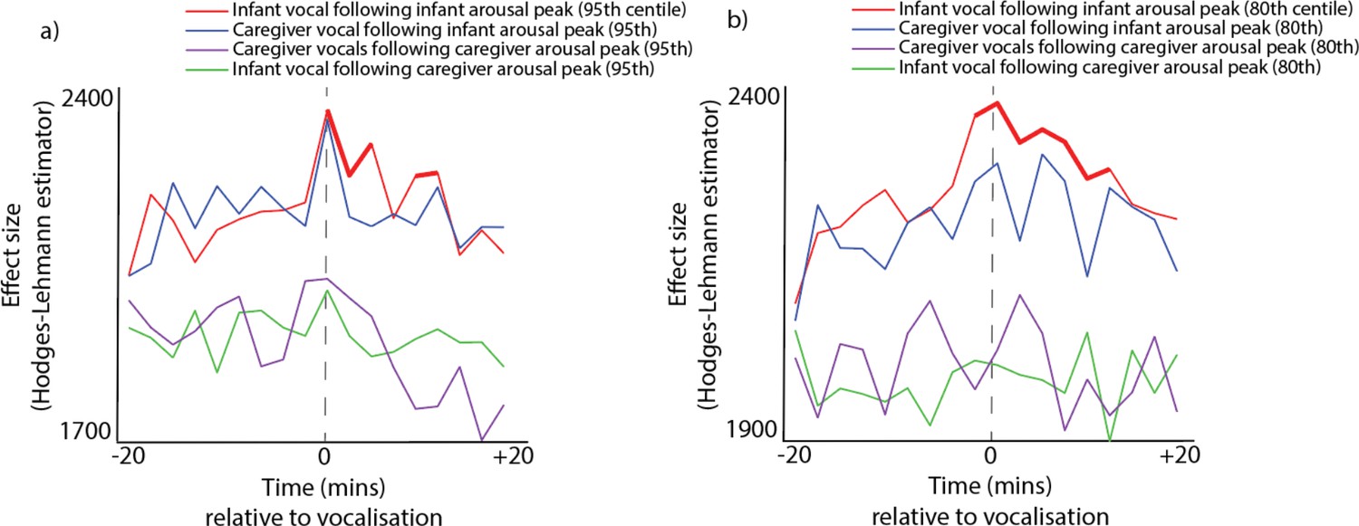
Identical to Figure 1f in the main text, except that different thresholds were used to define arousal peaks.
(a) shows the analysis repeated relative to 95th centile arousal peaks; (b) shows the analysis repeated relative to 80th centile arousal peaks.
Appendix 1—figure 8
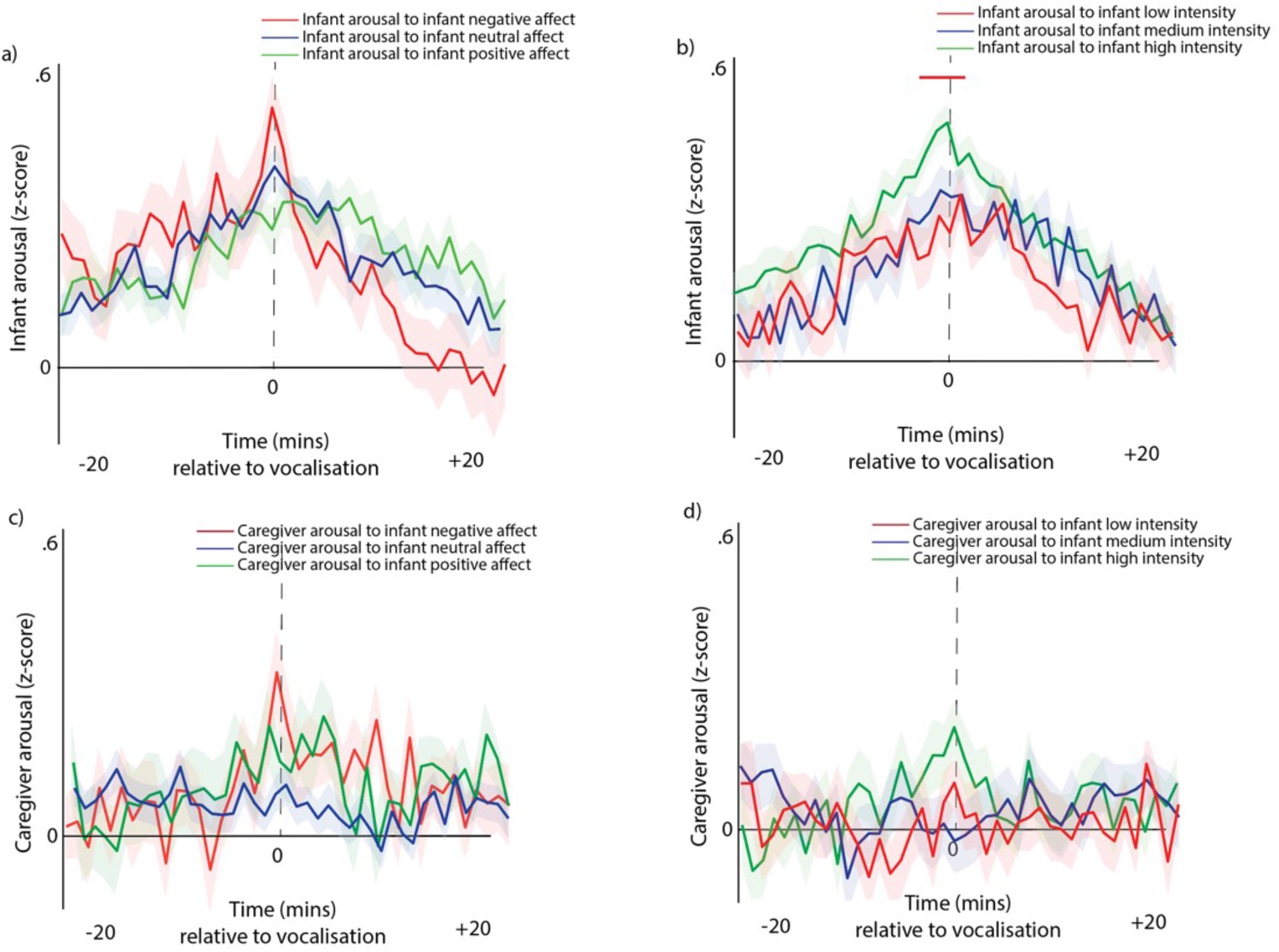
Arousal changes around vocalisations subdivided by infant vocalisation affect and intensity.
(a) Infant arousal around infant vocalisations, subdivided by infant vocal valence. (b) Infant arousal around infant vocalisations, subdivided by infant vocal intensity. (c) Identical to a, but examining the change in caregiver arousal, subdivided infant vocal affect. (d) Identical to b, but examining the change in caregiver arousal, subdivided by infant vocalisation intensity. For all plots, shaded areas indicate standard error, and red highlights indicate areas of significant difference after correction for multiple comparisons.
Appendix 1—figure 9
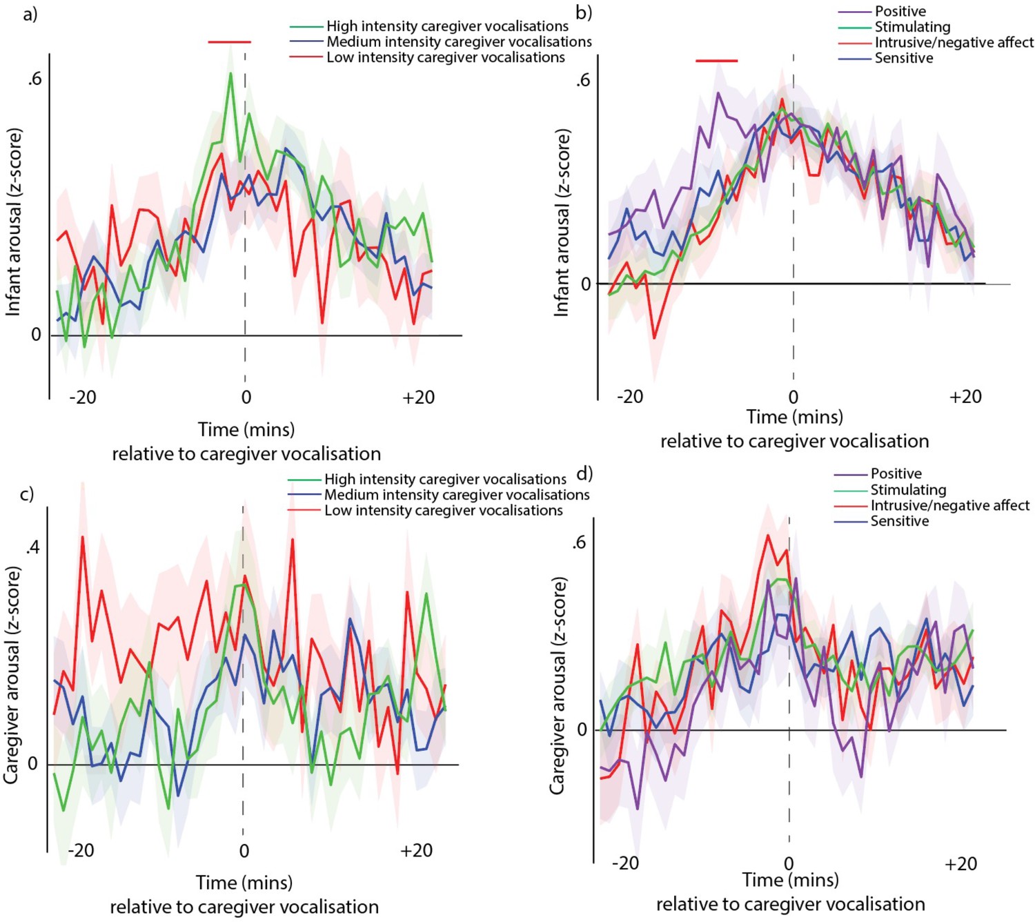
Arousal changes around vocalisations subdivided by adult vocalisation affect and intensity.
(a) Infant arousal around caregiver vocalisations, subdivided caregiver vocalisation intensity. (b) Infant arousal around caregiver vocalisations, subdivided by caregiver vocalisation type. (c) Identical to a, but examining the change in caregiver arousal, subdivided caregiver vocalisation intensity. (d) Identical to b, but examining the change in caregiver arousal, subdivided by caregiver vocalisation type. For all plots, shaded areas indicate standard error, and red highlights indicate areas of significant difference after correction for multiple comparisons (Figs a and b only).
Appendix 1—figure 10
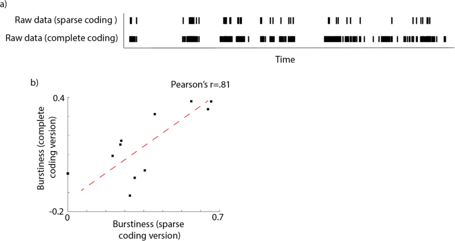
Examination of how sparse sampling affected the temporal distribution of our data.
(a) Example raw data file comparing a 2-hr long segment of fully coded data (containing all vocalisations recorded, based on continuous recording) with a ‘sparse coding’ simulation (containing just the vocalisations recording during the first 5 s of every minute). (b) We obtained N=10 continuous hour-long recordings from 5- to 10-month-old infants and examined the temporal distribution of the data, comparing the continuous recording with the sparse coding simulation described in (b). To quantify the temporal distribution of the data we calculated the burstiness (following the equation used in Abney et al., 2018). Scatterplot shows the relationship between the burstiness as estimated from the complete coding version and from the sparse coding version. The Pearson’s r between the two measures was r(9)=0.81, p<.001.
Author response image 1

Tables
Appendix 1—table 1
Demographic details for the sample (N=82).
| Infant age (days) – mean | 351.9 | |
|---|---|---|
| - SE | 4.6 | |
| Gender (% male) | 39.3 | |
| Infant Ethnicity (%) | White British | 51.9 |
| Other white | 11.4 | |
| Afro-Caribbean | 8.9 | |
| Asian, Indian & Pakistani | 10.1 | |
| Mixed - White/Afro-Carib | 2.5 | |
| Mixed - White/Asian | 7.6 | |
| Other mixed | 7.6 | |
| Household Income (%) | Under £16 k | 30.4 |
| £16-£25 k | 29.1 | |
| £26-£35 k | 11.4 | |
| £36-£50 k | 12.7 | |
| £51-£80 k | 8.9 | |
| >£80 k | 7.6 | |
| Maternal education (%) | Postgraduate | 34.2 |
| Undergraduate | 49.4 | |
| FE qualification | 2.5 | |
| A-level | 3.8 | |
| GCSE | 5.1 | |
| No formal qualifications | 2.5 | |
| Other | 1.3 | |
Additional files
Download links
A two-part list of links to download the article, or parts of the article, in various formats.
Downloads (link to download the article as PDF)
Open citations (links to open the citations from this article in various online reference manager services)
Cite this article (links to download the citations from this article in formats compatible with various reference manager tools)
Vocal communication is tied to interpersonal arousal coupling in caregiver-infant dyads
eLife 11:e77399.
https://doi.org/10.7554/eLife.77399


