The spatiotemporal patterns of major human admixture events during the European Holocene
Figures
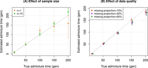
Simulation results.
We constructed n admixed individuals with 20% European (CEU) and 80% African (YRI) ancestry using ~380,000 genome-wide SNPs for admixture dates ranging between 10 and 200 generations. To minimize any issues with overfitting, we used French and Yoruba from the Human Genome Diversity Panel as reference populations in DATES (Distribution of Ancestry Tracts of Evolutionary Signals). We show the true time of admixture (X-axis, in generations) and the estimated time of admixture (±1 SE) (Y-axis, in generations). Standard errors were calculated using a weighted block jackknife approach by removing one chromosome in each run (Materials and methods). (A) Effect of sample size: We varied the sample size (n) of target group between 1 and 10 individuals. (B) Effect of data quality: To mimic the features of ancient genomes, we generated n=10 target individuals with pseudo-haploid genotypes and missing genotype rate as 10% (orange), 30% (purple), and 60% (green). See Figure 1—figure supplements 1–9 for additional simulations to test the performance of DATES. R code to replicate this figure is available at: https://github.com/manjushachintalapati/DATES_EuropeanHolocene/blob/main/1.R.
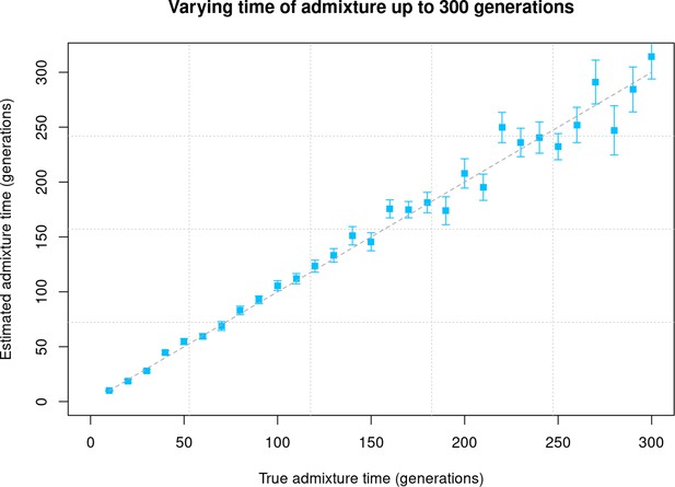
Varying time of admixture up to 300 generations.
We simulated data for 10 admixed individuals with 20% European (CEU) and 80% African (YRI) ancestry and varied the time of admixture between 10 and 300 generations. The X-axis shows the true time of admixture, and the Y-axis shows the estimated time of admixture (±1 SE) inferred using DATES (Distribution of Ancestry Tracts of Evolutionary Signals).
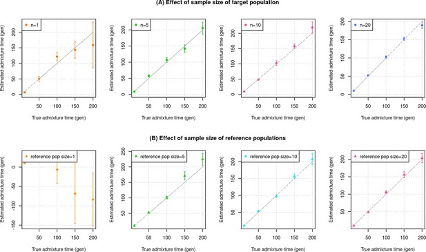
Impact of sample size of the target (admixed) and reference populations.
We simulated admixed individuals with 20% European (CEU) and 80% African (YRI) ancestry and applied DATES with m reference samples of French and Yoruba ancestry. (A) Effect of sample size of target population. Each panel shows the results of simulations with n target individuals shown in the legend and m=28 French and m=21 Yoruba reference samples from each source group. (B) Effect of sample size (m) of reference populations. Each panel shows the results of simulations with n=10 target individuals and m reference samples from each source group shown in the legend. The true admixture time is shown on X-axis, and the estimated time of admixture (±1 SE) is shown on Y-axis.
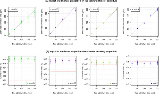
Impact of admixture proportion.
We simulated data for 10 admixed individuals with European (CEU) ancestry (α) in the range of 1–40% (the rest derived from Africans). We ran DATES (Distribution of Ancestry Tracts of Evolutionary Signals) to infer the time of admixture and ancestry proportion. (A) Impact on the estimated time of admixture: Each panel shows the estimated date of admixture for a different value of shown in the legend. The true admixture time is shown on X-axis, and the estimated time of admixture (±1 SE) is shown on Y-axis. (B) Impact on estimated ancestry proportion: Each panel shows the estimated proportion of admixture for a different value of shown in the legend. The red dashed horizontal line further indicates the value of used. The true time of admixture is shown on X-axis with the inferred proportion of admixture on Y-axis.
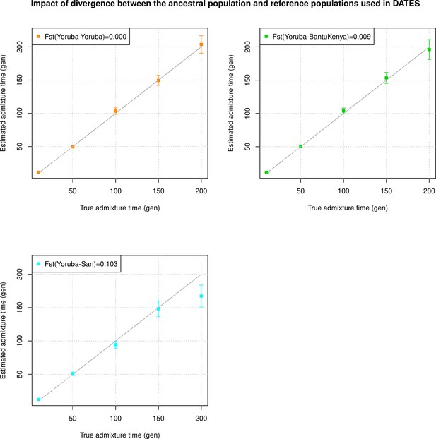
Impact of divergence between the ancestral population and reference populations used in DATES (Distribution of Ancestry Tracts of Evolutionary Signals).
We simulated 10 admixed individuals with 80% European (CEU) and 20% African (YRI) ancestry. We applied DATES to infer the timing of admixture using reference populations. In each panel, we show the estimated dates of admixture using French and a group that is increasingly divergent from Yoruba (shown in the legend as the FST with Yoruba). The true admixture time is shown on X-axis, and the estimated time of admixture (±1 SE) is shown on Y-axis.
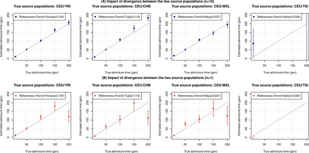
Impact of divergence between the two source populations.
We simulated n admixed individuals with 20% European (CEU) and 80% ancestry from a range of populations with increasing relatedness to Europeans (shown in the legend as the FST to Europeans). Specifically, the other reference population we used was either West Africans (YRI), East Asians (CHB), South Americans (MXL) or Southern Europeans (TSI). We used the following reference populations for the inference: French (for all simulations) with one of the other references as either Yoruba, Tujia, Maya, or Italian, respectively. We show results for varying target sample sizes of (A) n=10 and (B) n=1. The true admixture time is shown on X-axis, and the estimated time of admixture (±1 SE) is shown on Y-axis. We note the inferred dates for CEU/TSI mixtures were not significant for older timescales and hence not shown.
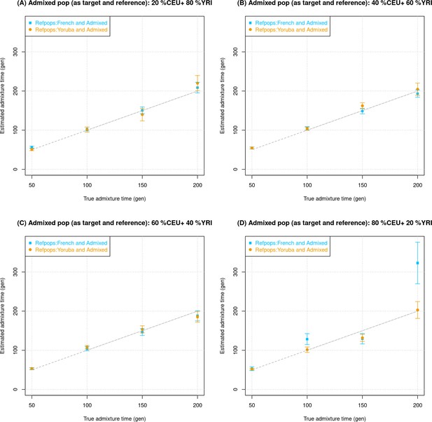
Impact of using the admixed individuals themselves as one of the reference groups in DATES (Distribution of Ancestry Tracts of Evolutionary Signals).
We simulated data for 10 admixed individuals with European (CEU) ancestry () in the range of 20–80% (the rest derived from Africans [YRI]) using CEU and YRI as reference populations. Using a non-overlapping set of CEU and YRI individuals, we generated 10 additional individuals that we used as reference samples in DATES. For each simulation, we ran DATES with Europeans (French) and a non-overlapping set of simulated admixed individuals as the reference populations (shown in blue), or Yoruba and simulated admixed individuals (shown in orange). The true admixture time is shown on X-axis, and the estimated time of admixture (±1 SE) is shown on Y-axis.
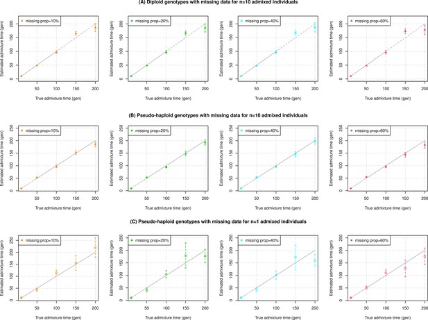
Impact of sample size and data quality of target samples.
We simulated data for n admixed individuals with 20% European (CEU) and 80% African (YRI) ancestry. In each panel, we varied three key features of the data from the target population, notably sample size (n=1 or 10), type of genotypes (diploid or pseudo-haploid) and missing genotype rate (between 10% and 60%). (A) Diploid genotypes with missing data for n=10 admixed individuals. Each panel shows the results of x% of missing diploid genotypes (shown in the legend). (B) Pseudo-haploid genotypes with missing data for n=10 admixed individuals. Each panel shows the results of x% of missing pseudo-haploid genotypes (shown in the legend). (C) Pseudo-haploid genotypes with missing data for n=1 admixed individuals. Each panel shows the results of x% of missing pseudo-haploid genotypes (shown in the legend). The true admixture time is shown on X-axis, and the estimated time of admixture (±1 SE) is shown on Y-axis.
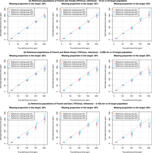
Impact of data quality of target and reference populations as a function of divergence between true and reference populations used in DATES (Distribution of Ancestry Tracts of Evolutionary Signals).
We simulated data for n=10 admixed individuals with 20% European (CEU) and 80% African (YRI) ancestry with pseudo-haploid genotypes. The reference populations used also had pseudo-haploid genotypes. We further varied three key features of the data, missing genotype rate in reference populations, missing genotype rate in target populations, and divergence between true source populations and reference population used for the analysis. In each row, we show the admixture dates using reference populations with increasing divergence to true source population (FST shown in the row title). In each column, we varied the missing genotype rate in the target population (shown in the column title). Further, each panel shows results of missing data in the reference genomes (shown in the legend). (a) Reference populations of French and Yoruba (FST(true, reference)~0). (b) Reference populations of French and Bantu Kenya (FST(true, reference)~0.009). (c) Reference populations of French and San (FST(true, reference)~0.103). The true admixture time is shown on X-axis, and the estimated time of admixture (±1 SE) is shown on Y-axis.
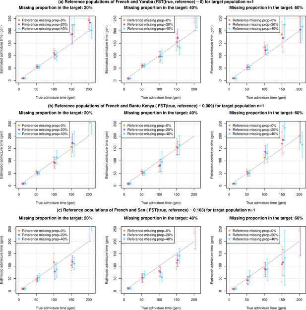
Impact of small sample size and data quality of target and reference populations as a function of divergence between true and reference populations used in DATES (Distribution of Ancestry Tracts of Evolutionary Signals).
We simulated data for n=1 admixed individuals with 20% European (CEU) and 80% African (YRI) ancestry with pseudo-haploid genotypes. The reference populations used also had pseudo-haploid genotypes. We further varied three key features of the data, missing genotype rate in reference populations, missing genotype rate in target populations, and divergence between true source populations and reference population used for the analysis. In each row, we show the admixture dates using reference populations with increasing divergence to true source population (FST shown in the row title). In each column, we varied the missing genotype rate in the target population (shown in the column title). Further, each panel shows results of missing data in the reference genomes (shown in the legend). (a) Reference populations of French and Yoruba (FST(true, reference)~0). (b) Reference populations of French and Bantu Kenya (FST(true, reference)~0.009). (c) Reference populations of French and San (FST(true, reference)~0.103). The true admixture time is shown on X-axis, and the estimated time of admixture (±1 SE) is shown on Y-axis.
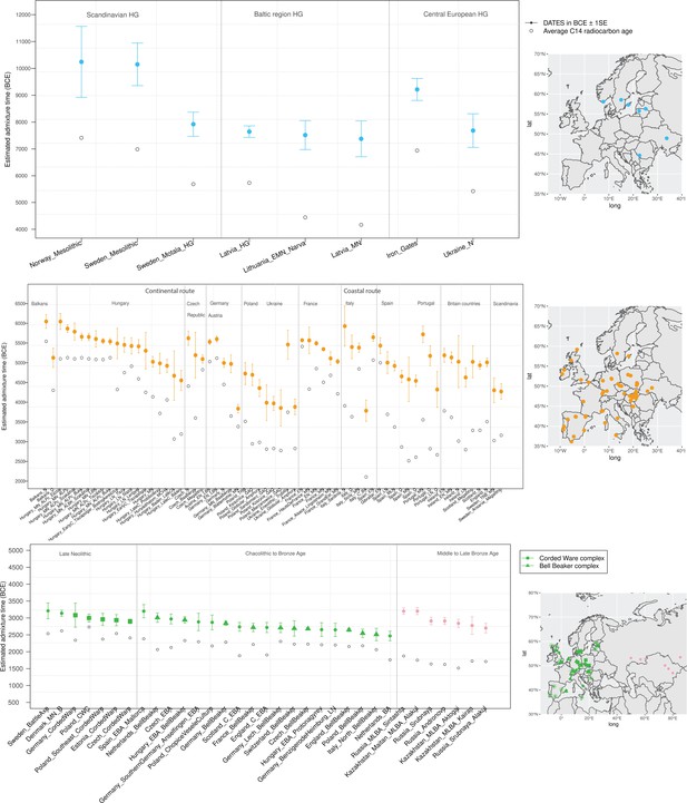
Timeline of admixture events in ancient Europe.
We applied DATES (Distribution of Ancestry Tracts of Evolutionary Signals) to ancient samples from Europe. In the right panel, we show the sampling locations of the ancient specimens, and in the left panel, we show the admixture dates for each target group listed on the X-axis. The inferred dates in generations were converted to dates in BCE by assuming a mean generation time of 28 years (Moorjani et al., 2011) and accounting for the average sampling age (shown as gray dots) of all ancient individuals in the target group (Materials and methods). The top panel shows the formation of western hunter-gatherer (WHG)-eastern hunter-gatherer (EHG) cline (in blue) using Mesolithic hunter-gatherers (HGs) as the target and EHG and WHG as reference populations. The middle panel shows admixture dates of local HGs and Anatolian farmers (in orange) using Neolithic European groups as targets and Anatolian farmers-related groups and WHG-related groups as reference populations. The bottom panel shows the spread of Steppe pastoralist-related ancestry (in green) estimated using middle and late Neolithic, Chalcolithic, and Bronze Age samples from Europe as target populations and early Steppe pastoralist-related groups (Afanasievo and Yamnaya Samara) and a set of Anatolian farmers and WHG-related groups as reference populations. For the middle to late Bronze Age (MLBA) samples from Eurasia, we used the early Steppe pastoralist-related groups and the Neolithic European groups as reference populations. The cultural affiliation (Corded Ware Complex [CWC], Bell Beaker complex [BBC], or Steppe MLBA cultures) of the individuals is shown in the legend. See Figure 2—figure supplements 1 and 2 we applied DATESfor decay curves for all samples and stratified datesfor Iron Gates HGs. R code to replicate this figure is available at: https://github.com/manjushachintalapati/DATES_EuropeanHolocene/blob/main/3.R.
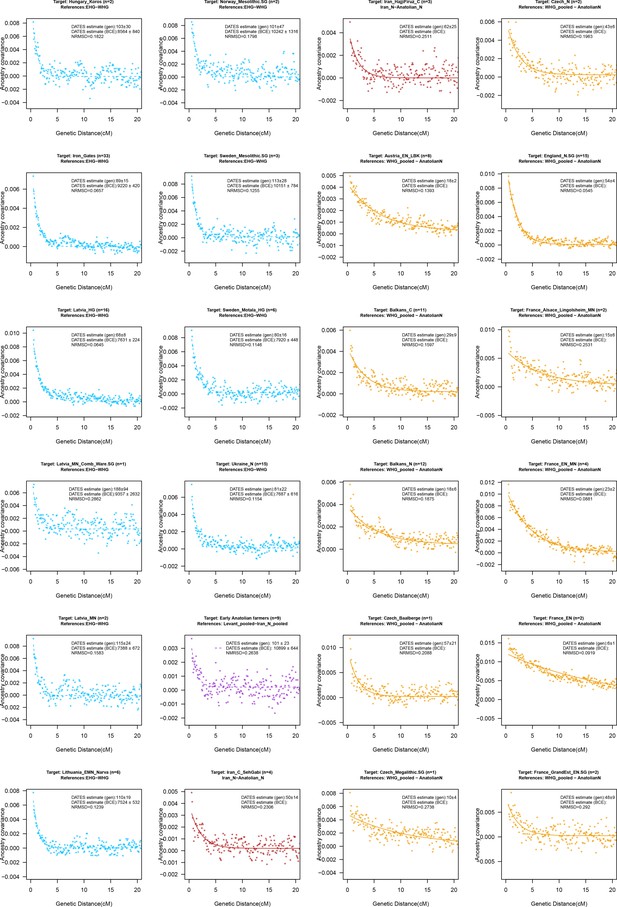
DATES (Distribution of Ancestry Tracts of Evolutionary Signals) ancestry covariance decay curves.
We show the weighted ancestry covariance decay curves generated using DATES for all the target groups analyzed in the study. Each subplot shows the decay curve for one target population with the associated reference groups shown in the title. For each target, in the legend, we show the inferred average dates of admixture (±1 SE) in generations before the individual lived, in BCE that accounts for the average age of all the individuals in the target and the mean generation time of human populations (see Materials and methods). We also show the normalized root-mean-square deviation (NRMSD) values for all fitted curves and the plots with NRMSD >0.7 are shown in gray. For consistency, we use the same colors as Figure 2.
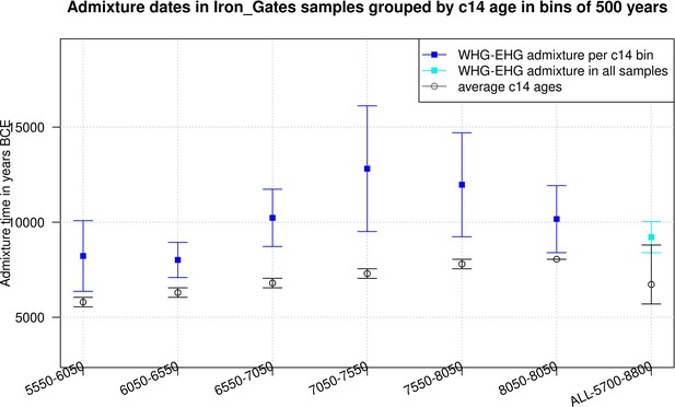
Timing of western hunter-gatherer (WHG) and eastern hunter-gatherer (EHG) admixture in Iron Gates hunter-gatherer (HG) samples.
The time of admixture in Iron Gates HG samples grouped in bins of C14 age of 500 years. The C14 age is shown on X-axis and the admixture time in BCE for corresponding samples is shown on the Y-axis.
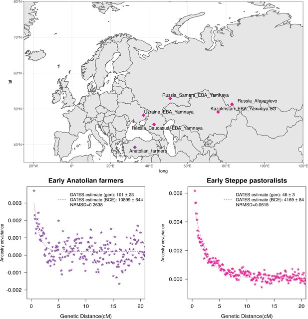
Genetic formation of early Anatolian farmers and early Bronze Age Steppe pastoralists.
The top panel shows a map with sampling locations of the target groups analyzed for admixture dating. The bottom panels show the inferred times of admixture for each target using DATES (Distribution of Ancestry Tracts of Evolutionary Signals) by fitting an exponential function with an affine term , where d is the genetic distance in Morgans and = (t+1) is the number of generations since admixture (t) (Materials and methods). We start the fit at a genetic distance (d) >0.5 cM (centiMorgans) to minimize confounding with background LD and estimate a standard error by performing a weighted block jackknife removing one chromosome in each run. For each target, in the legend, we show the inferred average dates of admixture (±1 SE) in generations before the individual lived, in BCE accounting for the average age of all the individuals and the mean human generation time, and the normalized root-mean-square deviation (NRMSD) values to assess the fit of the exponential curve (Materials and methods). The bottom left shows the ancestry covariance decay curve for early Anatolian farmers inferred using one reference group as a set of pooled individuals of western hunter-gatherer (WHG)-related and Levant Neolithic farmers-related individuals as a proxy of Anatolian hunter-gatherer (AHG) ancestry and the second reference group containing Iran Neolithic farmer-related individuals. The bottom right shows the ancestry covariance decay curve for early Steppe pastoralists groups, including all Yamnaya and Afanasievo individuals as the target group and eastern hunter-gatherer (EHG)-related and Iran Neolithic farmer-related groups as reference populations. R code to replicate this figure is available at: https://github.com/manjushachintalapati/DATES_EuropeanHolocene/blob/main/2.R.
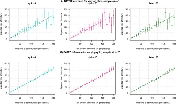
Impact of the discretization parameter (qbin) on accuracy.
We show three subplots for a sample size of n=1 (Panel A) and n=20 (Panel B). For each subplot, we simulated data for n admixed individuals with 20% ancestry from Europeans (1000 Genomes, CEU) and 80% ancestry from Africans (1000 Genomes, YRI) with the time of admixture () shown on the X-axis and the estimated admixture time inferred using DATES on Y-axis. We ran DATES using varying qbin values shown in different colors.
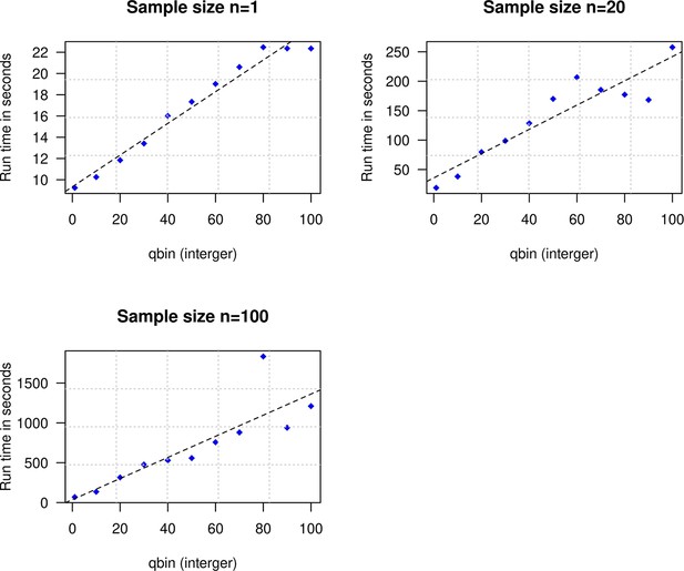
Impact of the discretization parameter (qbin) on runtime.
We show three subplots for sample size of n=1 (top left), n=20 (top right), and n=100 (bottom). For each subplot, we simulated data for n admixed individuals with 20% ancestry from Europeans (1000 Genomes, CEU) and 80% ancestry from Africans (1000 Genomes, YRI) with the time of admixture () of 100 generations ago. We show the impact of qbin (X-axis) on the runtime measured in seconds. For sample sizes, n>1, r2 between qbin and runtime is >0.99.
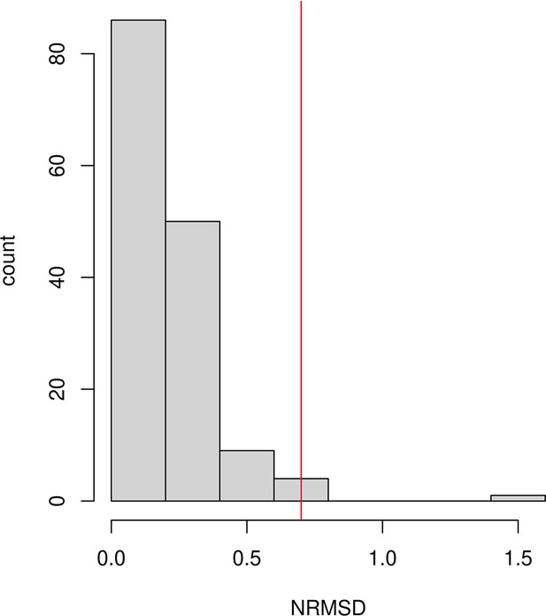
Histogram of the normalized root-mean-square deviation (NRMSD) values computed as the normalized residual between the empirical and fitted decay curves, for all the ancient DNA populations reported in Figure 2—figure supplement 1.
The red vertical line represents the value NRMSD = 0.7, which we used as the threshold to exclude populations from our analysis because visual inspection of fitted curves above this threshold suggests the results are too noisy to make a reliable inference (see Figure 2—figure supplement 1 for all fitted decay curves).
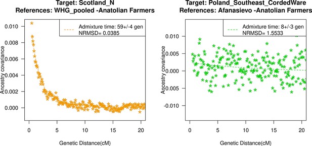
Ancestry covariance curves for the lowest (left) and highest (right) NRMSD values in our ancient DNA populations in our study.
For details of all curves and NRMSD estimation, see Figure 2—figure supplement 1.
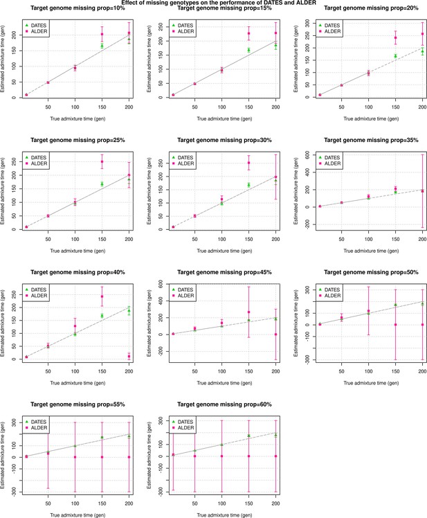
Effect of missing genotypes on the performance of DATES (Distribution of Ancestry Tracts of Evolutionary Signals) and ALDER: We simulated data for 10 admixed individuals with varying proportions of missing data (shown in each panel).
The estimated admixture times (±1 SE) from DATES (green) and ALDER (pink) are shown on Y-axis and the true time of admixture is shown on X-axis. For a fair comparison with ALDER, the dates reported here for DATES are using exponential fit to generations (instead of the default of λ generations).
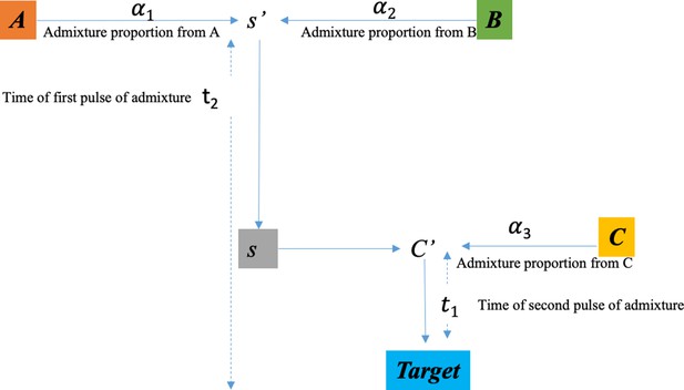
Model for multiple pulses of admixture.
The admixed population (Target) derives ancestry from three populations, from the two gene flow events that occurred generations ago (older pulse) between PopA and PopB with / ancestries respectively resulting in an intermediate group S, which then mixes with PopC with ancestry at 1 generations ago (younger pulse).
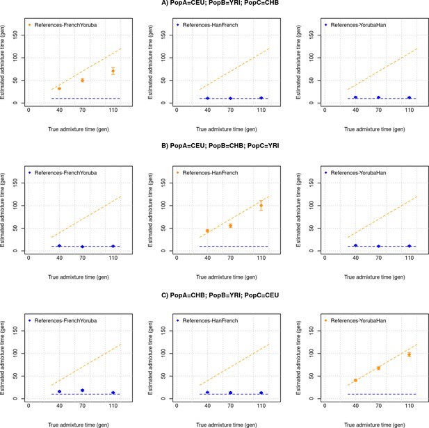
Multiple pulses of admixture with equal proportions of ancestry from sources.
We generated a target population that has ancestry from three groups (PopA, PopB, PopC) with ancestry proportions of 33%, 33%, and 33% respectively that mixed at two distinct times (t1=30,60,100 and t2=10 generations ago). We used CEU, YRI, and CHB as PopA, PopB, and PopC and varied the order of the three ancestrals, and applied DATES with pairs of populations as the reference to infer the timing of the mixture. We show the expected dates (t1 or t2 depending on the references used), the orange dashed line corresponds to the older pulse and the blue dashed line corresponds to the younger pulse of admixture. The blue points correspond to DATES estimates using PopA and PopC or PopB and PopC as references. The orange points correspond to DATES estimates using PopA and PopB as references. Panel (A) shows the admixture scenario with PopA = CEU, PopB = YRI, and PopC = CHB. Panel (B) shows the admixture scenario with PopA = CEU, PopB = CHB, and PopC = YRI, and Panel (C) shows the admixture scenario with PopA = CHB, PopB = YRI, and PopC = CEU.
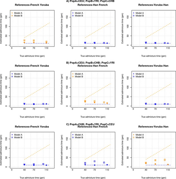
Two pulses of admixture with unequal proportions of ancestry from reference populations.
We generated a target population that has ancestry from three groups with variation in ancestry from three sources. Model A: PopA, PopB, PopC with ancestry proportion of 4%, 16%, and 80% respectively that mixed at two distinct times (t1=30,60,100 and t2=10 generations ago). Model B: PopA, PopB, PopC with ancestry proportion of 16%, 64%, and 20% respectively that mixed at two distinct times (t1=30,60,100 and t2=10 generations ago). We used CEU, YRI, and CHB as PopA, PopB, and PopC and varied the order of the three ancestral populations, and applied DATES with pairs of populations as the reference to infer the timing of the mixture. Figures shows the true time of admixture on the X-axis and inferred time on Y-axis, the orange dashed line corresponds to the older pulse and the blue dashed line corresponds to the younger pulse of admixture. The blue points correspond to DATES estimates using PopA and PopC or PopB and PopC as references. The orange points correspond to DATES estimates using PopA and PopB as references. Panel (A) shows the admixture scenario with PopA = CEU, PopB = YRI, and PopC = CHB. Panel (B) shows the admixture scenario with PopA = CEU, PopB = CHB, and PopC = YRI. Panel (C) shows the admixture scenario with PopA = CHB, PopB = YRI, and PopC = CEU.
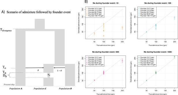
Impact of founder events on inferred dates of admixture.
(A) Schematic for demographic scenario shows that PopC was formed through admixture between PopA and PopB at time TA. Following admixture, PopC experienced a severe bottleneck that occurred TB generations ago where the effective population size decreased from 12,500 to NB for a duration of DB generations. After TB, the population recovered to the original population size. (B) We simulated data for 10 individuals with admixture occurring at 50, 100, and 200 generations with bottleneck post-admixture for a period of B = 1, 5, or 10 generations (shown in the legend) with the effective population size during bottleneck as NB = 10, 100, 500, or 1000 individuals (shown as four panels). The true admixture time is shown on X-axis, and the estimated time of admixture (±1 SE) is shown on Y-axis.
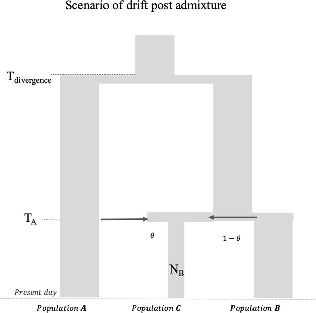
Impact of founder event with no recovery in admixed population.
Schematic for the demographic history of the admixed group PopC that has ancestry from PopA and PopB followed by a severe bottleneck post-admixture without recovery to present (i.e., maintenance of historically low population size to present NB). The FST (PopA, PopC) is 0.202 and FST (PopB, PopC) is 0.168.
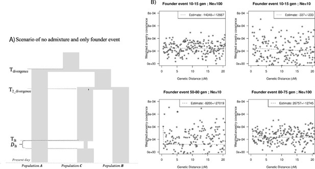
Impact of models with no admixture, severe founder event.
(A) Demographic scenario with three populations. PopA and PopB diverged 1800 generations ago and PopB and PopC diverged 1000 generations ago. PopC had a bottleneck at TB generations ago with population size during bottleneck NB. (B) Ancestry covariance curves for PopC. We simulated data for 25 individuals from PopA and PopB and 10 individuals from PopC. We applied DATES (Distribution of Ancestry Tracts of Evolutionary Signals) on PopC with PopA and PopB as sources and show the decay curves for different timing and effective population size of founder events. Note, none of the simulations show significant exponential fits and all dates include 0 in the estimated CI.
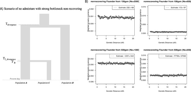
Effect of drift, no admixture: impact of models with no admixture, severe founder event (without recovery).
(A) Demographic scenario with three populations. PopA and PopB diverged 1800 generations ago and PopB and PopC diverged 1000 generations ago. PopC had a bottleneck at TB generations ago with population size during bottleneck NB. The population size NB is maintained to present. (B) Ancestry covariance curves for PopC. We simulated data for 25 individuals from PopA and PopB and 10 individuals from PopC. We applied DATES (Distribution of Ancestry Tracts of Evolutionary Signals) on PopC with PopA and PopB as sources and show the decay curves for different timing and effective population size of founder events.
Tables
Comparison of results using DATES (Distribution of Ancestry Tracts of Evolutionary Signals) v753 and v4010 using simulated data.
| (A) Simulated data with the target sample size (n) of 10 individuals | |||
|---|---|---|---|
| True time of admixture (generations) | DATES (V753) (mean ± SE) | DATES (v4010) (mean ± SE) | |
| 10 | 10.0±0.5 | 11.0±0.6 | |
| 20 | 19.1±1.5 | 19.6±1.5 | |
| 30 | 28.0±1.5 | 28.9±1.3 | |
| 40 | 46.1±2.1 | 45.7±1.8 | |
| 50 | 55.5±2.9 | 55.6±2.8 | |
| 60 | 59.4±2.2 | 60.5±2.4 | |
| 70 | 69.3±4.2 | 69.8±4.0 | |
| 80 | 84.2±4.4 | 84.0±3.9 | |
| 90 | 97.7±3.7 | 93.7±3.6 | |
| 100 | 107.4±5.4 | 106.7±4.5 | |
| 110 | 113.6±5.5 | 112.9±4.7 | |
| 120 | 122.7±5.4 | 124.3±5.5 | |
| 130 | 138.6±7.7 | 134.1±6.2 | |
| 140 | 153.2±9.2 | 152.0±8.4 | |
| 150 | 147.5±9.0 | 146.6±8.2 | |
| 160 | 181.4±9.8 | 176.6±8.2 | |
| 170 | 178.0±8.1 | 175.9±7.4 | |
| 180 | 180.7±10.6 | 182.3±9.3 | |
| 190 | 172.9±15.3 | 174.8±12.7 | |
| 200 | 204.7±17.1 | 208.8±13.4 | |
| 210 | 194.5±13.3 | 196.3±11.9 | |
| 220 | 255.8±17.0 | 250.7±13.8 | |
| 230 | 251.9±18.6 | 237.0±13.0 | |
| 240 | 234.7±18.3 | 241.5±14.2 | |
| 250 | 228.3±13.8 | 233.2±11.9 | |
| 260 | 254.2±21.7 | 253.0±16.1 | |
| 270 | 291.4±22.4 | 292.1±20.0 | |
| 280 | 252.4±25.2 | 248.1±22.4 | |
| 290 | 277.9±22.4 | 285.4±20.5 | |
| 300 | 318.6±23.3 | 315.1±20.3 | |
| (B) Simulated data with sample size (n) ranging between 10 and 20 individuals. | |||
| True time of admixture (generations) | Sample size | DATES (V753) (mean ±SE) | DATES (v4010) (mean ±SE) |
| 10 | 1 | 6.9±2.5 | 7.8±2.6 |
| 10 | 5 | 8.8±0.8 | 9.9±0.8 |
| 10 | 10 | 9.9±1.2 | 10.8±1.2 |
| 10 | 15 | 10.9±0.7 | 11.8±0.7 |
| 10 | 20 | 10.3±0.6 | 11.3±0.6 |
| 50 | 1 | 51.7±7.1 | 51.5±7.5 |
| 50 | 5 | 59.7±3.5 | 58.6±3.2 |
| 50 | 10 | 48.7±2.7 | 50.1±2.7 |
| 50 | 15 | 54.2±2.1 | 54.7±2.1 |
| 50 | 20 | 52.9±1.9 | 53.1±1.9 |
| 100 | 1 | 124.5±17.6 | 122.5±13.2 |
| 100 | 5 | 107.2±7.6 | 108.2±7.5 |
| 100 | 10 | 103.3±7.7 | 100.1±3.8 |
| 100 | 15 | 99.4±4.5 | 103.4±3.3 |
| 150 | 1 | 136.4±29.2 | 144.2±26.3 |
| 150 | 5 | 142.6±11.4 | 143±11.7 |
| 150 | 10 | 156.9±9 | 158.6±7 |
| 150 | 15 | 142.9±7.8 | 146.1±6.7 |
| 150 | 20 | 156.5±5.4 | 152.9±4.3 |
| 200 | 1 | 195.4±88.4 | 160.2±73.9 |
| 200 | 5 | 210.9±20.7 | 206.7±18.7 |
| 200 | 10 | 225±18.7 | 219.8±18 |
| 200 | 15 | 200±10.6 | 197.7±9 |
| 200 | 20 | 189.4±11 | 190.3±9 |
Comparison of results with Narasimhan et al., 2019.
| Population | Reference populations* | DATES (v753) | DATES (v4010) |
|---|---|---|---|
| (mean ±SE; in generations) | (mean ±SE; in generations) | ||
| Indus_Periphery_Pool | AASI and Iranian-farmer-related | 71±15 | 62±7 |
| SPGT | AASI and Steppe-pastoralist-related | 26±3 | 28±3 |
-
*
We used the reference populations of AASI ancestry that includes South Asians from the 1000 Genomes Project (Phase 3) including Sri Lankan Tamil from the UK (STU.SG) and Indian Telugu from the UK (ITU.SG), as well as BIR.SG, and Iranian farmer-related ancestry including Aigyrzhal_BA, Sarazm_EN, Geoksyur_EN, Parkhai_Anau_EN, and Steppe-pastoralist-related including Central_Steppe_MLBA.
Comparison of dates of the spread of Neolithic farming from Rivollat et al., 2020.
| Population | n | DATES (v753) | Population in our study (v44 1240K) | n (v44 1240K) | DATES (v4010)# |
|---|---|---|---|---|---|
| Bulgaria_MP_Neolithic | 9 | 8.4±2.3 | Bulgaria_MalakPreslavets_N | 8.05±3 | |
| Serbia_Neolithic | 4 | – | Serbia_EN | 22.8±9.8 | |
| Romania_EN | 2 | 32.1±10.4 | Romania_EN* | 2 | 29.7±7.1 |
| Croatia_Impressa | 2 | – | Croatia_EN_Impressa | 2 | – |
| Hungary_ALPc_MN | 23 | 21.5±4.7 | Hungary_MN_ALPc | 21.9±1.6 | |
| Hungary_LBK_MN | 10 | 12.8±5.2 | Hungary_MN_LBK | 18.6±7.4 | |
| Hungary_ALBK_MN | 2 | 14.8±3.2 | Hungary_MN_ALBK_Szakalhat | 2 | 19.3±3.3 |
| Hungary_LN | 18 | 21.5±3.7 | Hungary_LN | 18 | 28.03±3.8 |
| Austria_LBK_EN | 8 | 15.5±4.6 | Austria_EN_LBK | 17.6±2.3 | |
| Czech_MN | 5 | 18.3±7.7 | Czech_MN | 32.9±6.3 | |
| France_MN | 3 | 26.5±5.6 | France_MN | 30±1.3 | |
| Iberia_EN | 10 | 15.6±2.5 | Spain_EN | 20.6±3.6 | |
| Iberia_MN | 7 | 52.4±4.3 | Spain_MLN | 56.3±4 | |
| Germany_LBK_EN | 27 | 14.4±2.6 | Germany_EN_LBK | 17.4±2.7 | |
| Germany_Blatterhohle_MN | 4 | 12.3±2.5 | Germany_Blatterhohle_MN | 4 | 16.2±2.9 |
| Germany_Esperstedt_MN | 1 | – | Germany_MN_Esperstedt | 1 | – |
| England_Neolithic | 29 | 45.5±5.5 | England_N.SG | – | |
| Wales_Neolithic | 6 | 45.3±7.4 | Wales_N | 50.7±3.3 | |
| Scotland_Neolithic | 42 | 50.9±3.8 | Scotland_N | 56.6±2.9 | |
| Ireland_Neolithic | 13 | 46.9±7.5 | Ireland_MN.SG | 50.8±2.2 |
-
(Blue) indicates samples sizes that differ across both studies.
-
# For DATES (Distribution of Ancestry Tracts of Evolutionary Signals), we used pooled western hunter-gatherer (WHG) and Anatolian farmers as the reference populations except for samples marked with *.
-
*
Indicates cases where the results were not significant as the 95% CI includes 0.
Comparison of ALDER and DATES (Distribution of Ancestry Tracts of Evolutionary Signals) for varying samples sizes and times of admixture.
We simulated data for 20 and 100 admixed individuals using the CEU and YRI from 1000G with the mixture proportion of 20% from European and 80% African ancestry. The dates reported here for DATES are using exponential fit to generations.
| Time of admixture (gen) | Number of individuals, n=20 | Number of individuals, n=100 | ||
|---|---|---|---|---|
| ALDER mean ±1 SE (gen) | DATES mean ±1SE(gen) | ALDER mean ±1SE(gen) | DATES mean ±1SE(gen) | |
| 10 | 9.3±0.8 | 10.7±0.6 | 10.2±0.3 | 10±0.3 |
| 20 | 19.4±1.3 | 19.7±0.8 | 20.2±0.3 | 20.3±0.3 |
| 30 | 28.5±1.7 | 30.8±1.5 | 30.6±0.9 | 30.5±0.7 |
| 40 | 40.9±2 | 40.3±1.5 | 40.6±0.7 | 40.6±0.4 |
| 50 | 47.9±3.6 | 49.6±1.6 | 50±1.1 | 50.9±0.7 |
| 60 | 55.7±2.7 | 60.3±1.5 | 62±2.2 | 63.2±1 |
| 70 | 71.4±4 | 74±2.7 | 74±2.2 | 72.4±1.3 |
| 80 | 80.6±4.8 | 82.5±2.9 | 85.3±2.3 | 84.4±1.1 |
| 90 | 87.8±4.2 | 88.9±3 | 94.1±2.7 | 92.9±1.3 |
| 100 | 93.7±4.9 | 98.1±2.9 | 101.9±3.9 | 103.6±1 |
| 110 | 121.4±5.4 | 118.2±3.7 | 120.7±4.3 | 115.5±1.8 |
| 120 | 116.5±8.5 | 128.4±3.9 | 121.2±5.1 | 121.5±1.7 |
| 130 | 138.2±9.2 | 133.7±4.6 | 130.2±4.8 | 132.8±1.7 |
| 140 | 134.5±17.5 | 142.4±7 | 144.9±7.3 | 145.3±3.1 |
| 150 | 144.8±23.8 | 149.5±7.4 | 155.1±7 | 157.5±2.8 |
| 160 | 141.9±11.3 | 166.7±5.9 | 154.5±8.5 | 161.7±2.4 |
| 170 | 173.4±13.7 | 175.1±6.9 | 170.3±6.2 | 173.5±3 |
| 180 | 204.6±17.8 | 195.5±7.1 | 174.2±7 | 180.7±3.3 |
| 190 | 221.3±23.9 | 210.4±9.4 | 191.2±16.2 | 197.2±4.6 |
| 200 | 202.8±11.1 | 196±6.5 | 188.5±16.5 | 202.6±4.7 |
Admixture dates in present-day populations inferred using ROLLOFF, Globetrotter, ALDER, and DATES (Distribution of Ancestry Tracts of Evolutionary Signals).
| Population | nk | Source1 | Source2 | ROLLOFF | Globetrotter | ALDER formal test | ALDER_2-ref dates | DATES | Comments |
|---|---|---|---|---|---|---|---|---|---|
| Hazara | 22 | Mongola (10) | Iranian (13) | 23±1 | 22±0.9 | Long-range LD | -- | 24.6±1.0 | |
| Uzbekistani | 15 | Mongola (10) | Iranian (13) | 20±1.4 | 19±1.1 | SUCCEEDS | 19.18±2.22 | 21.3±1.4 | |
| Uyghur | 10 | Mongola (10) | Iranian (13) | 23±2.6 | 22±1.3 | SUCCEEDS | 16.73±1.38 | 22.2±2.1 | |
| Makrani | 22 | Bantu Kenya (11) | Balochi (21) | 18±1.8 | 18±1.2 | Long-range LD | -- | 13.2±1.6 | |
| Druze | 42 | Yoruba (21) | Cypriot (12) | 39±7.3 | 37±1.9 | FAILS | 44.02±6.37 | 43.4±6.1 | |
| Mozabite | 25 | Yoruba (21) | Moroccan (22) | 23±1.9 | 21±1.3 | Long-range LD | -- | 21.6±1.8 | |
| Turkish | 17 | Mongola (10) | Iranian (13) | 28±3.2 | 24±1.5 | FAILS | 25.62±2.48 | 28.5±2.3 | |
| Brahui | 23 | Bantu Kenya (11) | Balochi (21) | 13±3.4 | 20±1.5 | Long-range LD | -- | 10.4±1.6* | Possibly multi-way admixture (Pagani et al., 2017) |
| Yemeni | 4 | Bantu Kenya (11) | Syrian (16) | 15±2.3 | 14±1.8 | FAILS | 6.29±2.89 | 12.7±1.6 | |
| Pima | 14 | Turkish (17) | Mayan (21) | 9±3.6 | 6±0.9 | SUCCEEDS | 6.29±0.89 | 7.8±1.1 | |
| Bantu South Africa | 8 | San Khomani (30) | Yoruba (21) | 26±2.5 | 25±2.3 | Long-range LD | -- | 27.9±2.2 | |
| Tu | 10 | Greek (20) | Han N-China (10) | 33±6.3 | 25±2.3 | FAILS | 28.83±2.8 | 31.3±1.96 | |
| West Sicilian | 10 | Yoruba (21) | East Sicilian (10) | 26±7.8 | 27±3.9 | FAILS | 42.72±16.34 | 37.4±16.4 | |
| Cambodian | 10 | Uyghur (10) | Han (34) | 17±4.7 | 20±2.7 | SUCCEEDS | 24.28±5.36 | 33.6±3.7* | |
| Georgian | 20 | Adygei (17) | Greek (20) | -- | 30±3.3 | FAILS | 3.15±1.22 | -- | |
| Romanian | 13 | Lithuanian (10) | East Sicilian (10) | -- | 31±2.6 | FAILS | -- | -- | |
| Bulgarian | 18 | Polish (16) | Cypriot (12) | -- | 28±3.5 | FAILS | 40.95±16.42 | 91.1±24.7* | Possibly multi-way admixture or different model of admixture (see Main text and Haak et al., 2015) |
| Hezhen | 8 | Tujia (10) | Mongola (10) | -- | 13±1.3 | FAILS | 2.92±1.4 | -- | |
| Oroqen | 9 | Yakut (25) | Mongola (10) | -- | 15±2 | Long-range LD | -- | -- | |
| Hungarian | 18 | Cypriot (12) | Polish (16) | 65±24 | 39±3.5 | FAILS | 54.83±25.27 | 61.8±19.1 | |
| Han N-China | 10 | Turkish (17) | Tujia (10) | 37±11.1 | 26±3.8 | FAILS | 48.17±10.36 | 44.3±5.1* | |
| Daur | 9 | Tujia (10) | Mongola (10) | -- | 21±1.7 | FAILS | -- | -- | |
| Greek | 20 | Polish (16) | Cypriot (12) | 69±18.5 | 36±3.7 | FAILS | 55.54±8.93 | 62.6±16.9 | |
| Melanesian | 10 | Papuan (16) | Cambodian (10) | 66±12.1 | 28±7.6 | FAILS | 64.91±5.42 | 68.6±7.1* | |
| Mandenka | 22 | Moroccan (22) | Yoruba (21) | 22±10.3 | 19±4.2 | FAILS | 17.25±6.05 | 85.8±19.0 *#Ω | Possibly multiple admixture events (Price et al., 2009) |
| Indian | 13 | Cambodian (10) | Sindhi (23) | 91±41.1 | 53±8.4 | FAILS | n/a | n/a | There are multiple “Indian” groups in the dataset making it unclear which target was used |
| North Italian | 12 | Cypriot (12) | French (28) | -- | 71±11.8 | FAILS | 12.44±4.32 | -- | |
| Polish | 16 | French (28) | Lithuanian (10) | -- | 31±5.1 | FAILS | -- | -- | |
| Tuscan | 8 | Cypriot (12) | French (28) | -- | 35±6.1 | FAILS | -- | -- | |
| San Namibia | 5 | Sandawe (28) | San Khomani (30) | -- | 48±8.9 | Long-range LD | -- | -- |
-
Columns 1–5 include results from Table S12 from Hellenthal et al., 2014. We only show significant dates (|Z| > 2).
-
Following Hellenthal et al., we created a merged dataset of the Human Genome Diversity Panel, Henn et al. and Behar et al. containing 1642 individuals and 465543 SNPs. This dataset was used for ALDER and DATES analysis.
-
Standard errors in DATES were estimated using chromosome jackknife (see Materials and methods).
-
-- indicates results where the inferred results were not significant, either the method failed or the 95% CI included 0.
-
* indicates DATES estimates that significantly differ from Globetrotter estimates (not within two SEs).
-
# indicates DATES estimates that significantly differ from ROLLOFF results.
-
Ω indicates DATES estimates that significantly differ from ALDER results.
-
n/a indicates target population was unclear.
Admixture dates for Neolithic European groups using DATES (Distribution of Ancestry Tracts of Evolutionary Signals) and modified ALDER (Lipson et al., 2017).
| Region | Population | Modified ALDER* (Lipson et al., 2017) | DATES† |
|---|---|---|---|
| Germany | Blätterhöhle_MN | 18.5±4.6 | 14±3 |
| Germany | Germany_MN | 26.2±4.4 | 36±20 |
| Germany | LBK_EN | 14.9±2.4 | 18±3 |
| Hungary | LBK_EN | 17.8±2.0 | 22±2 |
| Hungary | Baden_CA | 27.6±3.8 | 49±11 |
| Hungary | Lasinja_CA | 29.3±5.2 | 32±6 |
| Hungary | LBKT_MN | 30.3±5.8 | 23±10 |
| Hungary | Protoboleraz_CA | 44.3±6.4 | 46±7 |
| Hungary | Starcevo_EN | 4.5±1.9 | 5±2 |
| Hungary | TDLN | 20.9±2.7 | 29±4 |
| Hungary | Tisza_LN | 18.2±6.6 | 27±9 |
| Spain | Iberia_CA | 49.6±5.2 | 55±6 |
| Spain | Iberia_EN | 19.4±2.3 | 20±3 |
| Spain | Iberia_MN | 49.9±7.7 | 52±8 |
-
*
Modified ALDER – We report the individual level dates from Extended Data Table 4 based on average of individual level dates calculated using Anatolian farmers and western hunter-gatherer (WHG) as sources and high coverage Anatolian farmers as helper samples. For details, see Lipson et al., 2017
-
†
DATES – We used pooled WHG groups and Anatolian farmers as references in DATES.
Impact of reference populations in two-way admixed groups.
| Model: We generated target populations with two pulses of gene flow where PopA and PopB mixed at time t1 generations ago with ancestry proportion of 1 and 2, followed by gene flow from PopC at t2 generations ago with ancestry proportion of 3 | |||||||
|---|---|---|---|---|---|---|---|
| Target | t2/t1 | Ref1 | Ref 2 | 1=20%, 2=80%, 3=80% | 1=50%, 2=50%, 3=50% | 1=20%, 2=80%, 3=20% | 1=20%, 2=80%, 3=10% |
| (A) Using reference populations PopA and PopC | |||||||
| PopA = CEU PopB = YRI PopC = CHB | 100/10 | Han | French | 10.3 | 10.7 | 12.0 | 12.6 |
| PopA = CEU PopB = CHB PopC = YRI | 100/10 | Yoruba | French | 10.3 | 9.7 | 10.2 | 10.6 |
| PopA = CHB PopB = YRI PopC = CEU | 100/10 | French | Han | 10.8 | 11.6 | 20.7 | 44 |
| PopA = CEU PopB = YRI PopC = CHB | 60/10 | Han | French | 11.3 | 10.7 | 11.8 | 14.4 |
| PopA = CEU PopB = CHB PopC = YRI | 60/10 | Yoruba | French | 10.4 | 10.8 | 10.3 | 11.2 |
| PopA = CHB PopB = YRI PopC = CEU | 60/10 | French | Han | 11.2 | 12.6 | 19.9 | 40.7 |
| (B) Using reference populations PopB and PopC | |||||||
| PopA = CEU PopB = YRI PopC = CHB | 100/10 | Han | Yoruba | 10.2 | 11.5 | 11.3 | 11.9 |
| PopA = CEU PopB = CHB PopC = YRI | 100/10 | Yoruba | Han | 10.1 | 9.7 | 10.3 | 10.5 |
| PopA = CHB PopB = YRI PopC = CEU | 100/10 | French | Yoruba | 10.1 | 12.8 | 12.2 | 14 |
| PopA = CEU PopB = YRI PopC = CHB | 60/10 | Han | Yoruba | 11.0 | 12.6 | 12.2 | 14.6 |
| PopA = CEU PopB = CHB PopC = YRI | 60/10 | Yoruba | Han | 10.3 | 11.1 | 10.6 | 11.4 |
| PopA = CHB PopB = YRI PopC = CEU | 60/10 | French | Yoruba | 10.4 | 13.4 | 12.4 | 18 |
| (C) Using reference populations PopC and ‘admixed’ individuals with ancestry from PopA and PopB (30% PopA/70% PopB) ancestry | |||||||
| PopA = CEU PopB = YRI PopC = CHB | 100/10 | Han | Admixed (30% CEU/ 70% YRI) | 10.1 | 10.9 | 10.8 | 10.5 |
| PopA = CEU PopB = CHB PopC = YRI | 100/10 | Yoruba | Admixed (30% CEU/ 70% CHB) | 10.1 | 9.5 | 10.0 | 10 |
| PopA = CHB PopB = YRI PopC = CEU | 100/10 | French | Admixed (30% CHB/ 70% YRI) | 10.0 | 11.2 | 10.9 | 10.8 |
| PopA = CEU PopB = YRI PopC = CHB | 60/10 | Han | Admixed (30% CEU/ 70% YRI) | 11 | 11.3 | 10.9 | 11.8 |
| PopA = CEU PopB = CHB PopC = YRI | 60/10 | Yoruba | Admixed (30% CEU/ 70% CHB) | 10.3 | 10.8 | 10.3 | 10.5 |
| PopA = CHB PopB = YRI PopC = CEU | 60/10 | French | Admixed (30% CHB/ 70% YRI) | 10.2 | 11.3 | 10.6 | 12.1 |
| (D) Using reference populations PopC and pooled individuals of PopA and PopB ancestry | |||||||
| PopA = CEU PopB = YRI PopC = CHB | 100/10 | Han | French + Yoruba | 10.1 | 10.99 | 10.4 | 9.5 |
| PopA = CEU PopB = CHB PopC = YRI | 100/10 | Yoruba | French + Han | 10.2 | 9.5 | 10.03 | 9.9 |
| PopA = CHB PopB = YRI PopC = CEU | 100/10 | French | Han + Yoruba | 9.9 | 10.4 | 10.6 | 10 |
| PopA = CEU PopB = YRI PopC = CHB | 60/10 | Han | French + Yoruba | 10.9 | 10.8 | 10.3 | 10.3 |
| PopA = CEU PopB = CHB PopC = YRI | 60/10 | Yoruba | French + Han | 10.3 | 10.7 | 10.1 | 10.5 |
| PopA = CHB PopB = YRI PopC = CEU | 60/10 | French | Han + Yoruba | 10.0 | 10.3 | 9.8 | 11 |
-
Note: the estimated dates are shown per scenario are averages of 10 simulations.
Impact of continuous gene flow.
The table shows true and inferred times of admixture in PopC using PopA and PopB used as the reference populations.
| The true period of continuous admixture, generations | Inferred time of admixture (mean ±1 SE) is shown on Y-axis generations |
|---|---|
| 10–15 | 15±1 |
| 20–30 | 23±2 |
| 40–60 | 53±3 |
| 40–100 | 64±4 |
Admixture time estimates from DATES (Distribution of Ancestry Tracts of Evolutionary Signals) for populations with extreme bottlenecks with a historically low population size that does not recover until the present.
| Admixture | Ne before admixture | Ne post-admixture | Inferred time of admixture |
|---|---|---|---|
| 100 | 12,500 | 4000 | 96±5 |
| 3500 | 96±5 | ||
| 3000 | 88±4 | ||
| 2500 | 99±5 | ||
| 2000 | 92±6 | ||
| 1500 | 78±6 | ||
| 1000 | 86±6 | ||
| 500 | 54±9 | ||
| 100 | 42±10 |
Additional files
-
Supplementary file 1
Data and admixture dates inferred using DATES (Distribution of Ancestry Tracts of Evolutionary Signals) for European groups during the Holocene (Excel sheet).
(A) Information on ancient samples used in our study. (B) Estimated dates of admixture for population mixture events during the European Holocene.
- https://cdn.elifesciences.org/articles/77625/elife-77625-supp1-v2.xlsx
-
Supplementary file 2
Formal tests of admixture for populations in Europe using qpAdm and D-statistics with default parameters in ADMIXTOOLS (Excel sheet).
(A) Modeling population admixture of hunter-gatherer (HG) groups using qpAdm in ADMIXTOOLS. (B) D-statistics to assess the affinity of Mesolithic HG groups to western hunter-gatherers (WHGs) or Anatolian farmers. (C) Modeling population admixture of Near Eastern farmers using qpAdm in ADMIXTOOLS. (D) Modeling population admixture of Neolithic European groups using qpAdm in ADMIXTOOLS. (E) Modeling population admixture of Neolithic European groups per individual using qpAdm in ADMIXTOOLS. (F) D-statistics to explore the affinity of the target groups to Steppe pastoralists or Anatolian farmers. (G) Modeling population admixture of Early Steppe pastoralists groups using qpAdm in ADMIXTOOLS. (H) Genetic distance (FST) in early Steppe pastoralists groups. (I) Modeling population admixture of Bronze Age groups using qpAdm in ADMIXTOOLS. (J) Modeling population admixture of Bronze Age groups per individual using qpAdm in ADMIXTOOLS. (K) Modeling population admixture of middle to late Bronze Age (MLBA) Steppe pastoralists groups. Age groups using qpAdm in ADMIXTOOLS.
- https://cdn.elifesciences.org/articles/77625/elife-77625-supp2-v2.xlsx
-
Transparent reporting form
- https://cdn.elifesciences.org/articles/77625/elife-77625-transrepform1-v2.pdf


