Contribution of behavioural variability to representational drift
- Department of Bioengineering, Imperial College London, United Kingdom
Figures
Figure 1 with 5 supplements
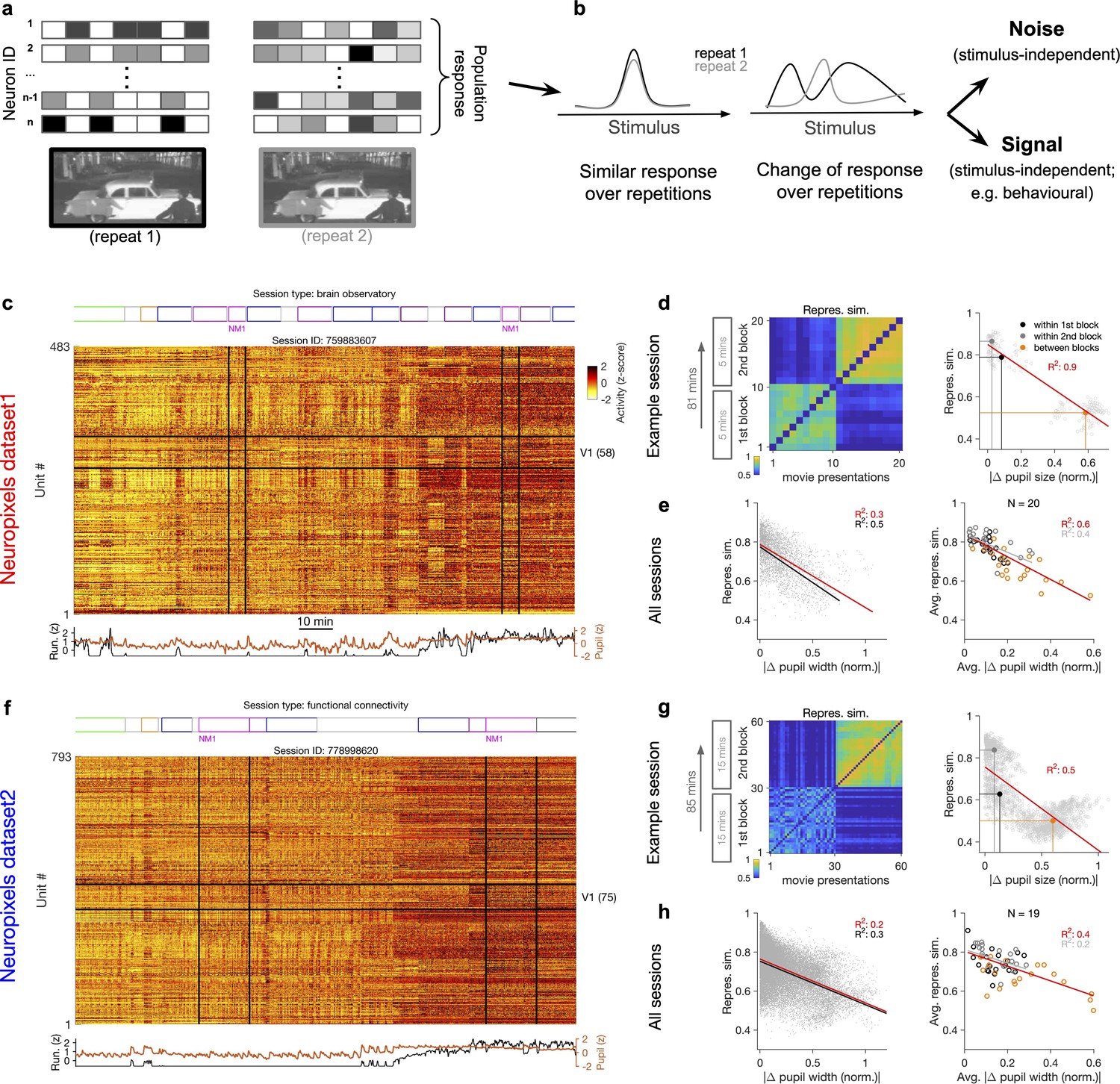
Representational similarity depends on the behavioural state of the animal.
(a) Illustration of the response of a population of neurons to a stimulus (e.g. a natural movie) which is shown twice (left versus right). (b) Neuronal response to different repetitions of the same stimulus can remain the same (left) or change from the original pattern (right), leading to a change in neural representations. This change can arise from an added stimulus-independent noise, which is randomly and independently changing over each repetition. Alternatively, it can be a result of another signal, which is modulated according to a stimulus-independent parameter (e.g. behaviour) that is changing over each repetition. (c) Population activity composed of activity of 483 units in an example recording session in response to different stimuli (timing of different stimulus types denoted on the top). Spiking activity of units is averaged in bins of 1 s and z-scored across the entire session for each unit. Units in primary visual cortex (V1; 58 units) and the two blocks of presentation of natural movie 1 (NM1) are highlighted by the black lines. Bottom: pupil size and running speed of the animal (z-scored). (d) Representational similarity between different presentations of NM1. It is calculated as the correlation coefficient of vectors of population response of V1 units to movie repeats (see ‘Methods’). Left: the matrix of representational similarity for all pairs of movie repeats within and across the two blocks of presentation. Right: representational similarity as a function of the pupil change, which is quantified as the normalized absolute difference of the average pupil size during presentations (see ‘Methods’). The best-fitted regression line (using least-squares method) and the R2 value are shown. Filled circles show the average values within and between blocks. (e) Same as (d) right for all recording sessions. Left: data similar to (d) grey dots are concatenated across all mice and the best-fitted regression line to the whole data is plotted. Black line shows the fit when movie repeats with significant change in the average running speed of the animal is considered (80th percentile). Right: the average values within and between blocks filled circles in (d) are plotted for all mice and the fitted regression line to these average values is plotted. Grey lines and R2 values indicate the fit to within-block data only. N: number of mice. (f–h) Same as (c–e) for a different dataset. Source data (for normalized changes in pupil width and representational similarity between pairs of movie repeats) are provided for individual sessions across the two datasets (Figure 1—source data 1).
-
Figure 1—source data 1
Related to Figure 1.
Source data (for normalized changes in pupil width and representational similarity between pairs of movie repeats) for individual sessions across the two Neuropixels datasets.
- https://cdn.elifesciences.org/articles/77907/elife-77907-fig1-data1-v2.xls
Figure 1—figure supplement 1
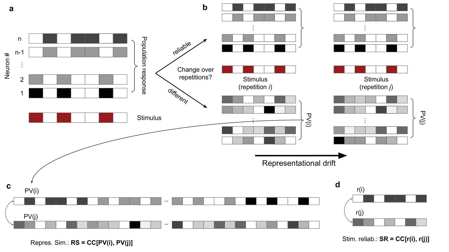
Characterization and quantification of representational similarity (RS) and representational drift.
(a) Left: illustration of response of a population of neurons (#1 to #n; upper) to a stimulus (lower), composed of binary values (ON: red; OFF: white). (b) The population response to two other repetitions of the same stimulus can remain the same (upper), demonstrating a stable and reliable code, or it can change from the original pattern (lower), leading to a drift of representations. Representational drift can be quantified by a representational drift index (RDI), which compares the correlation of population responses within the same session/block of presentation () with the correlation of population responses across sessions/blocks (; see ‘Methods’). (c) The degree of change or constancy of representations can be assayed by comparing the population responses to repeats of the same stimulus. The degree of similarity is quantified by RS, which is quantified by the correlation coefficient (CC) of the concatenated (across neurons) vector of population responses to two repeats (PV(i) and PV(j)). (d) Stimulus reliability (SR) is calculated for each unit individually, from the CC of the vector of responses of that unit to two stimulus presentations.
Figure 1—figure supplement 2
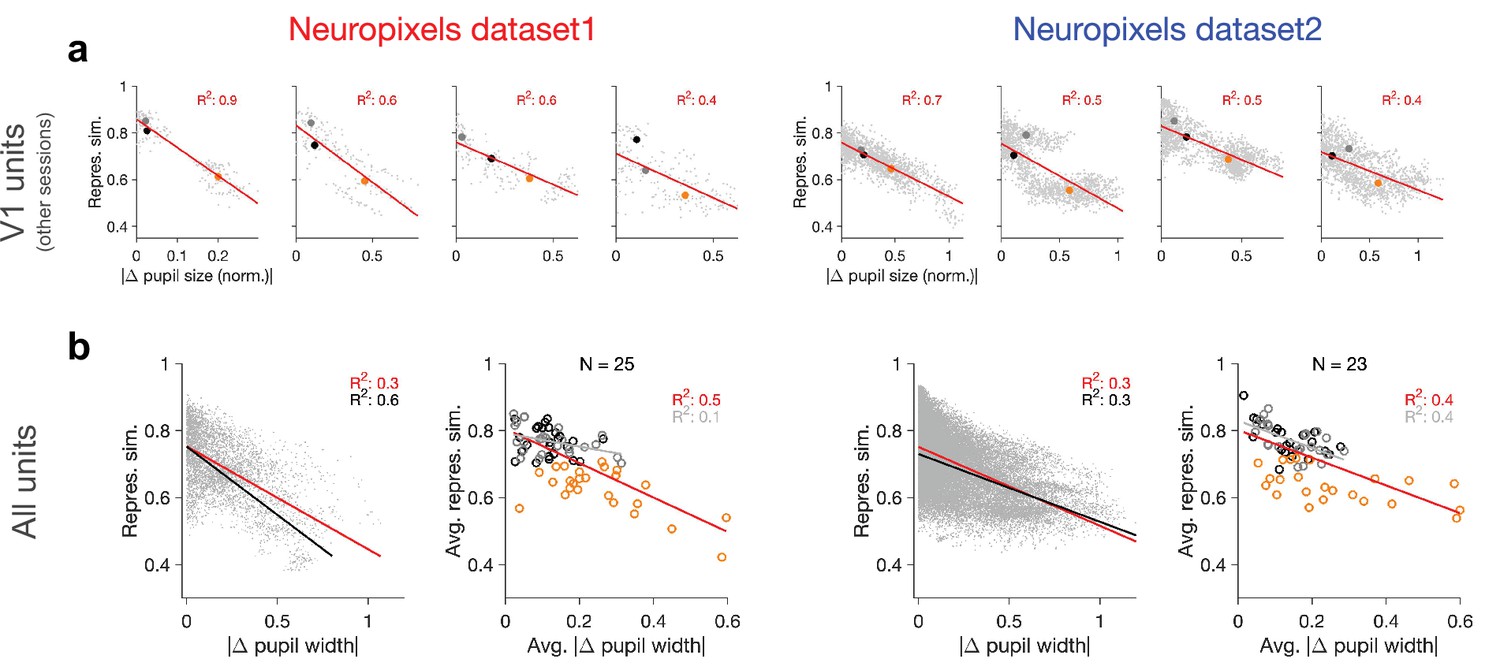
Relation between behavioural changes and representational similarity in other sessions and for all units.
(a) Same as Figure 1d and g for four other example recording sessions. Left: examples from Neuropixels dataset 1; session numbers and the number of V1 units (#), respectively: 762602078 (#75), 750332458 (#63), 760345702 (#72), 751348571 (#49). Left: examples from Neuropixels dataset 2; session numbers and the number of V1 units (#), respectively: 766640955(#52), 787025148(#68), 771990200(#54), 829720705(#52). Only sessions with #>40 units are included in the analysis. (b) Same as Figure 1e and h when all recorded units are included (instead of only V1 units).
Figure 1—figure supplement 3
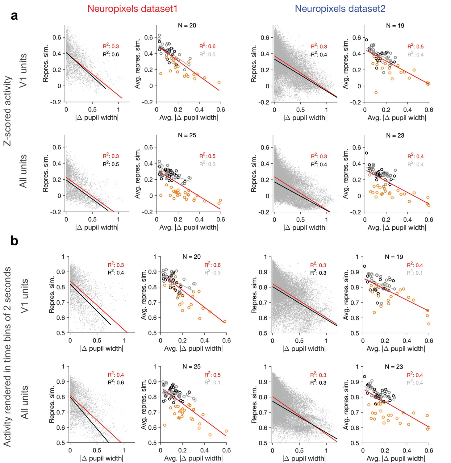
Dependence of representational similarity on behavioural change when calculated from z-scored activity and from activity rendered in longer time bins.
(a) Same as Figure 1e and h when population vectors are composed of z-scored activity of units in V1 (upper) or all regions (lower). Z-scored activity of unit is calculated as , where and are the average and SD of the activity of unit () during the two blocks of presentation of natural movie 1. Left: Neuropixels dataset 1; right: Neuropixels dataset 2. (b) Same as Figure 1e and h when representational similarity is calculated from the activity of units rendered in time bins of 2 s (instead of original 1 s; see ‘Methods’).
Figure 1—figure supplement 4
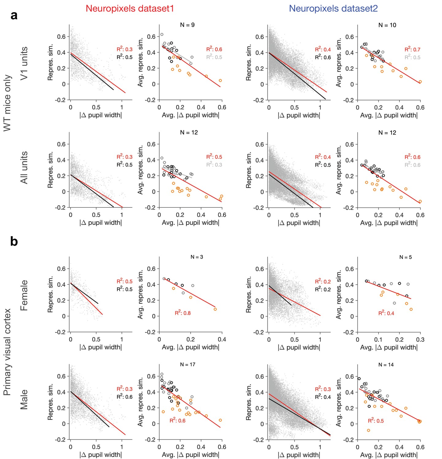
Dependence of representational similarity on behavioural change in wild-type (WT) mice and for male/female animals separately.
Same as Figure 1—figure supplement 2 when (a) only WT mice are included in the analysis or (b) when the analysis is performed for V1 units in female and male mice separately (see Supplementary file 1 for details). Left: Neuropixels dataset 1; right: Neuropixels dataset 2.
Figure 1—figure supplement 5
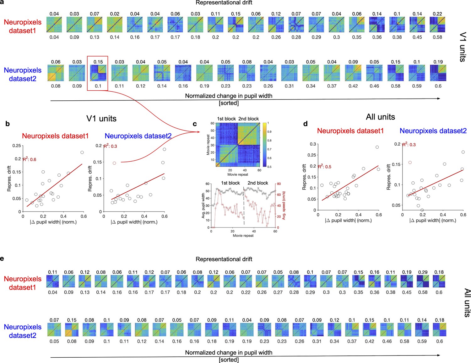
Representational drift between the two blocks of stimulus presentation in animals with different levels of behavioural variability.
(a) Matrices of representational similarity (calculated from population vectors of V1 units) between repeats of natural movie 1 (similar to Figure 1d and g, left) for sessions across the two datasets. Upper: Neuropixels dataset 1; lower: Neuropixels dataset 2; the colour code is the same as the example shown in (c). The numbers on the bottom denote the average change in the pupil width between the two blocks (average of the absolute normalized change between all pairs of repeats in the first and the second block), and the sessions are sorted according to that (from the least change to the highest change). The numbers on the top denote the representational drift index (RDI; see ‘Methods’) between the two blocks, which is calculated as , where and represent the average representational similarity within sessions and between sessions of the two blocks, respectively. is obtained as the average of average CC within the first block and the second block. (b) Relationship between the average change in pupil size (numbers denoted on the bottom of plots in a) and representational drift for different sessions in the two datasets. Red lines show the best-fitted regression lines, with values of R2 denoted in red. (c) The example session, highlighted with the red box in (a) is singled out (top), as being an outlier in terms of the relation between pupil change and RD between the two blocks red circle in (b). The average pupil width and running speed for each movie repeat is shown for this session on the bottom. (d, e) Same as (b, a) respectively, for all units (instead of V1 units).
Figure 2 with 3 supplements
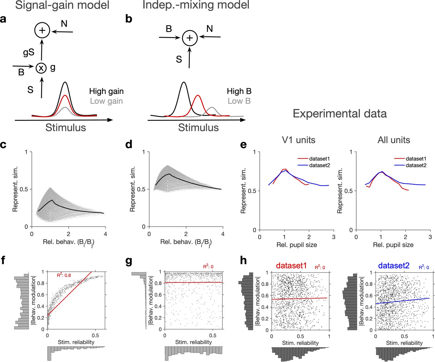
Independent modulation of activity by stimulus and behaviour.
(a) Schematic of a signal-gain model in which behaviour controls the gain with which the stimulus-driven signal is scaled. Individual units are driven differently with the stimulus, leading to different tuning curves which determines their stimulus signal, . Behavioural parameter, B, sets the gain, , with which the stimulus signal is scaled, before being combined with the noise term, N, to give rise to the final response. S is the same across repetitions of the stimulus, while N is changing on every repeat (see Figure 2—figure supplement 1a and ‘Methods’). (b) An alternative model (independent-mixing) in which the response of a unit is determined by the summation of its independent tuning to stimulus, S (red) and behaviour, B (black: high B; grey: low B), combined with noise, N (see ‘Methods’ for details). (c) Representational similarity of population responses to different repeats of the stimulus as a function of the relative behavioural parameter () in the signal-gain model. Black line shows the average (in 20 bins). (d) Same as (c), for the independent-mixing model. (e) Same as (c, d) for the experimental data from Neuropixels dataset 1 (red) or dataset 2 (blue). For each pair of movie repeats, the average representational similarity of population responses (left: V1 units; right: all units) are plotted against the relative pupil size (). (f, g) Relation between behavioural modulation and stimulus reliability of units in different models. The stimulus signal-gain model predicts a strong dependence between behavioural modulation and stimulus reliability of units (f), whereas the independent-mixing model predicts no correlation between the two (g). Best-fitted regression lines and R2 values are shown for each case. Marginal distributions are shown on each axis. (h) Data from V1 units in the two datasets show no relationship between the stimulus reliability of units and their absolute behavioural modulation, as quantified by the best-fitted regression lines and R2 values. Stimulus reliability is computed as the average correlation coefficient of each unit’s activity vector across repetitions of the natural movie, and behavioural modulation is calculated as the correlation coefficient of each unit’s activity with the pupil size (see ‘Methods’). Marginal distributions are shown. Source data (for stimulus reliability of V1 units and their modulation by pupil size) are provided for individual sessions across the two datasets (Figure 2—source data 1).
-
Figure 2—source data 1
Related to Figure 2.
Source data (for stimulus reliability of V1 units and their modulation by pupil size) for individual sessions across the two Neuropixels datasets.
- https://cdn.elifesciences.org/articles/77907/elife-77907-fig2-data1-v2.xls
Figure 2—figure supplement 1
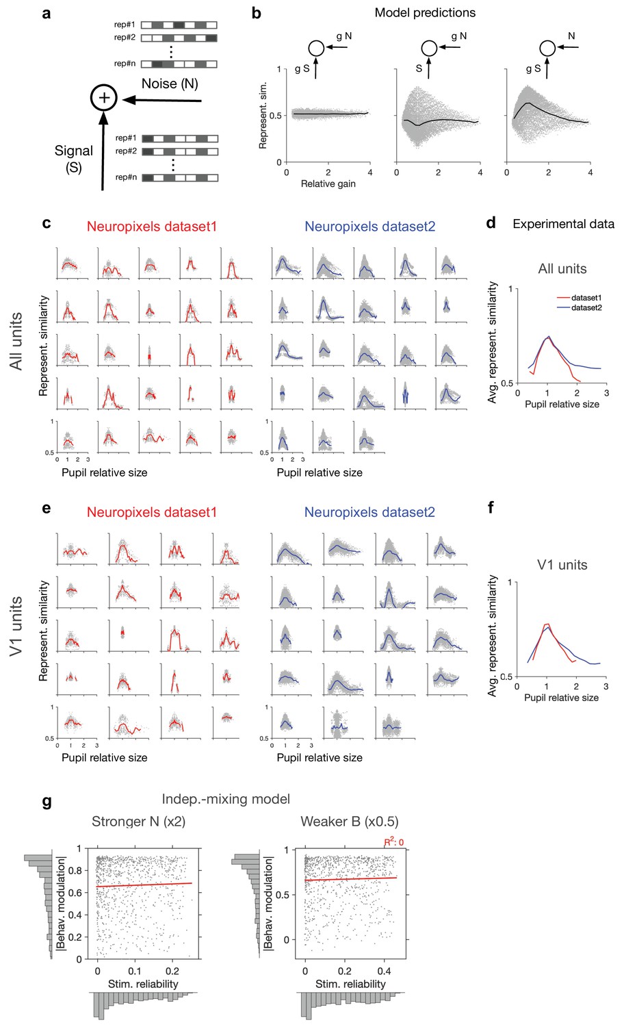
Dependence of representational similarity on behaviour in different gain models and in different experimental datasets.
(a) A model neuron which integrates the signal and the noise components in its inputs. The signal has the same pattern over multiple repetition (rep#) of the stimulus, while the noise changes in each repeat. (b) Representational similarity as a function of relative gain of the repeats ( , where and are the gains in the th and th repeats) for three models, where both signal and noise (left), only noise (middle), or only signal (right) components of the input are scaled by behaviour (see ‘Methods’ for details). Change in the gain did not change representational similarity when both signal and noise were scaled (left), consistent with our theoretical analysis (see ‘Methods’). When arousal scaled noise only, there was a small decrease in the average representational similarity (middle). The most prominent effect was observed when arousal scaled signal only. For this scenario, a general increase in the average representational similarity was obtained, with the maximum increase happening at equal gains () (right). (c) Representational similarity as a function of relative pupil size (obtained by the division of the average pupil sizes in a pair of movie repeats) for all recorded units. (d) The average representational similarity of all mice shown in (c) for datasets 1 (red) and 2 (blue) separately. Bottom: same when V1 units are only included, from the sessions with more than 40 units (the inclusion criterion). (e) Same as (c) when V1 units are only included in the analysis. There are fewer individual sessions here because not all sessions contained more than 40 V1 units. (f) Same as (d) for V1 units. (g) Same as Figure 1g, for a stronger value of noise (x2 N; left) or a weaker value of behavioural signal (x0.5 B; right).
Figure 2—figure supplement 2

Wide and mixed distribution of stimulus and behavioural modulations.
(a) Distribution of stimulus reliability for all V1 units from all sessions in Neuropixels dataset 1 (red) and dataset 2 (blue). The average stimulus selectivity for the two datasets are (0.32, 0.36), respectively. Grey lines show the distribution of stimulus reliability when it is calculated for each block separately and then average across the two blocks. The average values obtained in this manner are (0.36, 0.40) for the two datasets, respectively. (b) Sample activity of V1 units with high stimulus reliability (indicated by the numbers on the top) from each dataset. Top: the activity in response to each movie repeat; bottom: average activity in each block of presentation. (c) Distribution of behavioural modulation of all V1 units for the two datasets. Behavioural modulation is obtained as the correlation coefficient (CC) of each unit’s activity with pupil size. (d) Sample activity of V1 units with strong modulation by pupil size (numbers indicated on the top). Top: tuning of unit’s activity with pupil size. Bottom: the activity of units in response to repeats of the natural movie, showing different levels of modulation by stimulus within and across blocks of presentation (denoted by the value of stimulus reliability on top). (e, f) Activity of units can be weakly or strongly modulated by stimulus or behaviour, giving rise to four possible quadrants. Sample V1 units from each quadrant are shown for Neuropixels dataset 1 (e) and dataset 2 (f). For each sample, z-score activity of the unit across different repetitions of the movie is plotted (left), with the number on top denoting stimulus reliability of the unit. The average activity of each unit as a function of average pupil size (during each movie repeat) is plotted on the right, with the number on the top denoting behavioural modulation of the unit (CC with pupil size).
Figure 2—figure supplement 3
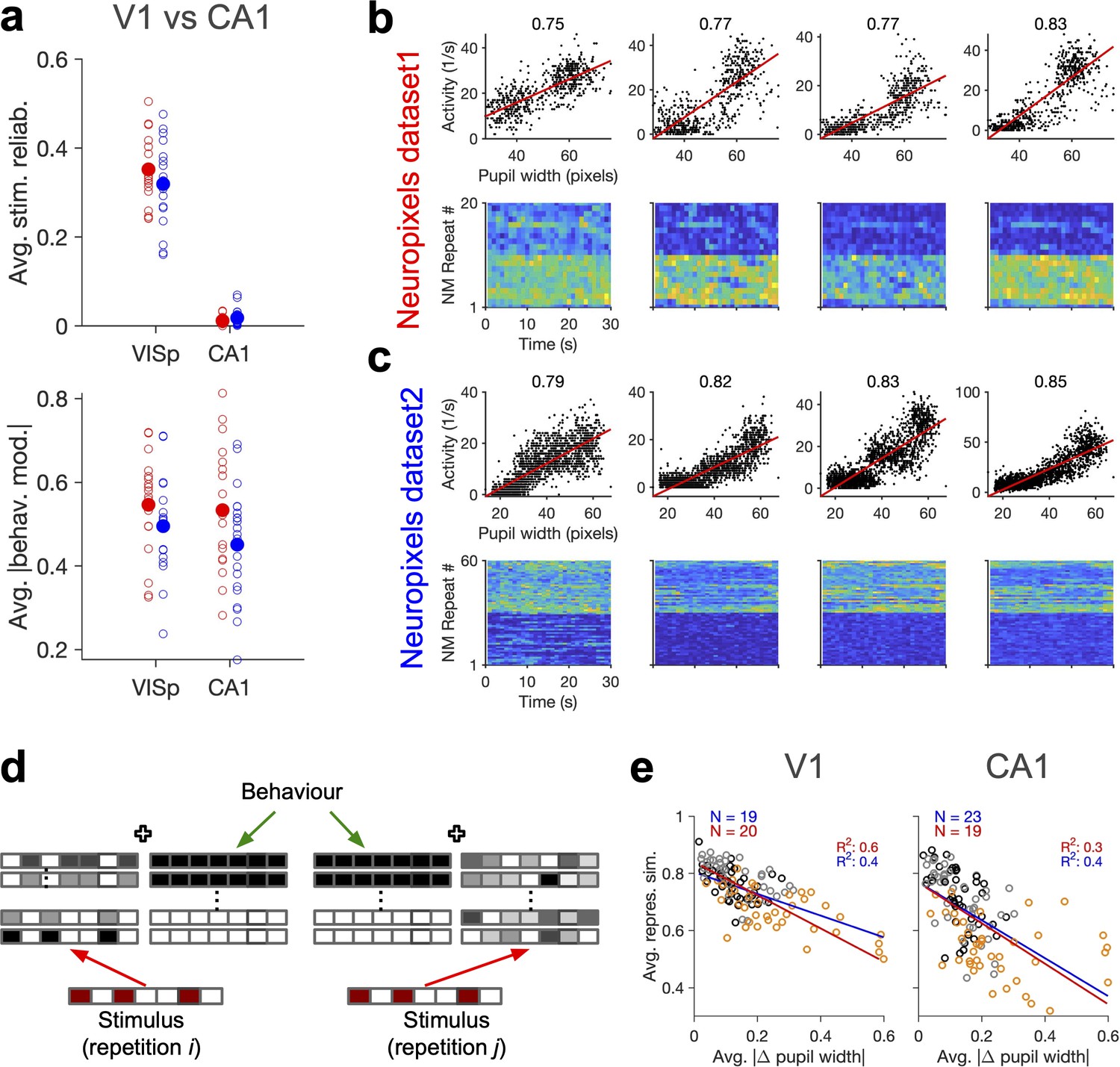
Stimulus-independent behavioural modulation of CA1.
(a) Top: average stimulus reliability across units in V1 and CA1 for different mice in each dataset. Bottom: same for the average (across units) of the absolute value of behavioural modulation. Filled circles: average across mice. Red: Neuropixels dataset 1; blue: Neuropixels dataset 2. (b) Top: sample activity of CA1 units (from Neuropixels dataset 1) with considerable modulation by pupil size (numbers indicated on the top). Bottom: the activity of units in response to repeats of the natural movie. (c) Same as (b) for Neuropixels dataset 2. (d) Schematic representation of population responses with stimulus-evoked (red) and behaviourally induced (green) components to the repeats of the same stimulus. Even if the stimulus-evoked component is different between repeats (red), the population vector of responses (see Figure 1—figure supplement 1c) can have some similarity due to the constancy of the component set by the behaviour (green). (e) Average representational similarity as a function of change in pupil width (similar to Figure 1e and h, right) for V1 (left) and CA1 units (right). Red: Neuropixels dataset 1; blue: Neuropixels dataset 2.
Figure 3 with 2 supplements

Behavioural variability modulates the low-dimensional components of population activity independent of stimulus reliability.
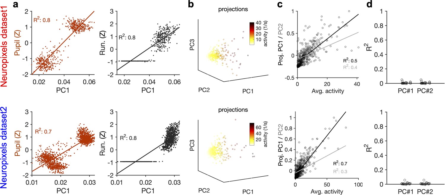
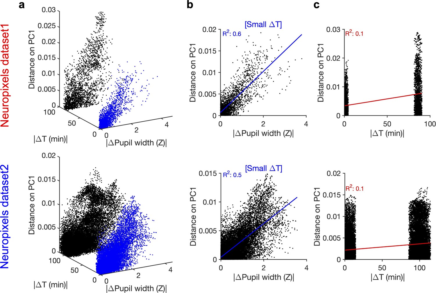
(a) Relative contribution of the first 10 principal components (PCs) of population responses to the variability of activity (quantified by the fraction of explained variance by each PC) for an example session (same as shown in Figure 1). (b) Population activity in the low-dimensional space of the first three PCs (see ‘Methods’ for details). Pseudo colour code shows the pupil size at different times, indicating that the sudden transition in the low-dimensional space of activity is correlated with changes in the behavioural state. (c) Projection of units’ activity over PC1 (black) or PC2 (grey) (respective PC loadings) versus stimulus reliability of the units. It reveals no correlation between the two, as quantified by best-fitted regression lines in each case (the best-fitted regression lines and R2 values shown by respective colours). PC loadings are normalized to the maximum value in each case. (d) Fraction of variance explained by PCs 1–3 for all sessions. (e) Distance on PC1 versus the difference of the average pupil size between different time points on the trajectory for all sessions. For each pair of non-identical time points on the PC trajectory, the absolute difference of PC1 components is calculated as the distance on PC and plotted against the absolute difference of the average pupil width (normalized by z-scoring across the entire session). Best-fitted regression line and the corresponding R2 value are shown in red for all data points, and in blue for data points with small time difference between the pairs (see Figure 3—figure supplement 2). (f) Same as (c) for all units from all sessions in dataset 1. (g–l) Same as (a–f) for Neuropixels dataset 2.
Figure 3—figure supplement 1
Relation of the principal components (PCs) of neural activity to the average activity of units and their stimulus reliability.
(a) Strong correlation between PC1 and the behavioural state of animal, as assayed by either pupil size (left) or running speed (right). Both pupil size and running speed are normalized by z-scoring across the entire session. (b) Projections of the activity of units in example sessions over the first three PCs (Figure 3a, b, g and h), with the average activity of each unit indicated by the pseudo colour code. (c) Projection of units’ activity over PC1/PC2 versus the average activity of the unit. The best-fitted regression lines and R2 values in each case are shown. (d) Similar to Figure 3c and i for individual sessions. R2 values of regression lines fitted to the projection of units’ activity over PC1/PC2 versus stimulus reliability of the respective units are plotted for individual sessions. Upper: Neuropixels dataset 1; lower: Neuropixels dataset 2.
Figure 3—figure supplement 2
Principal component (PC)1 and its relation to difference in pupil size and time.
(a) Relationship between distance on PC1 (Figure 3e and k), change in pupil width and passage of time. Data points highlighted in blue show the cluster with smaller passage of time (corresponding to movie repeats within the same blocks of presentation). Note that the two clusters arise from two blocks of stimulus presentation, which are separated from each other for >80 min in both datasets. (b) Distance on PC1 versus change in pupil width for data points with small passage of time (blue data points in a). The best-fitted regression line and its R2 value are denoted in blue. (c) Distance on PC1 versus passage of time. The best-fitted regression line and its R2 value are denoted in red.
Figure 4 with 5 supplements
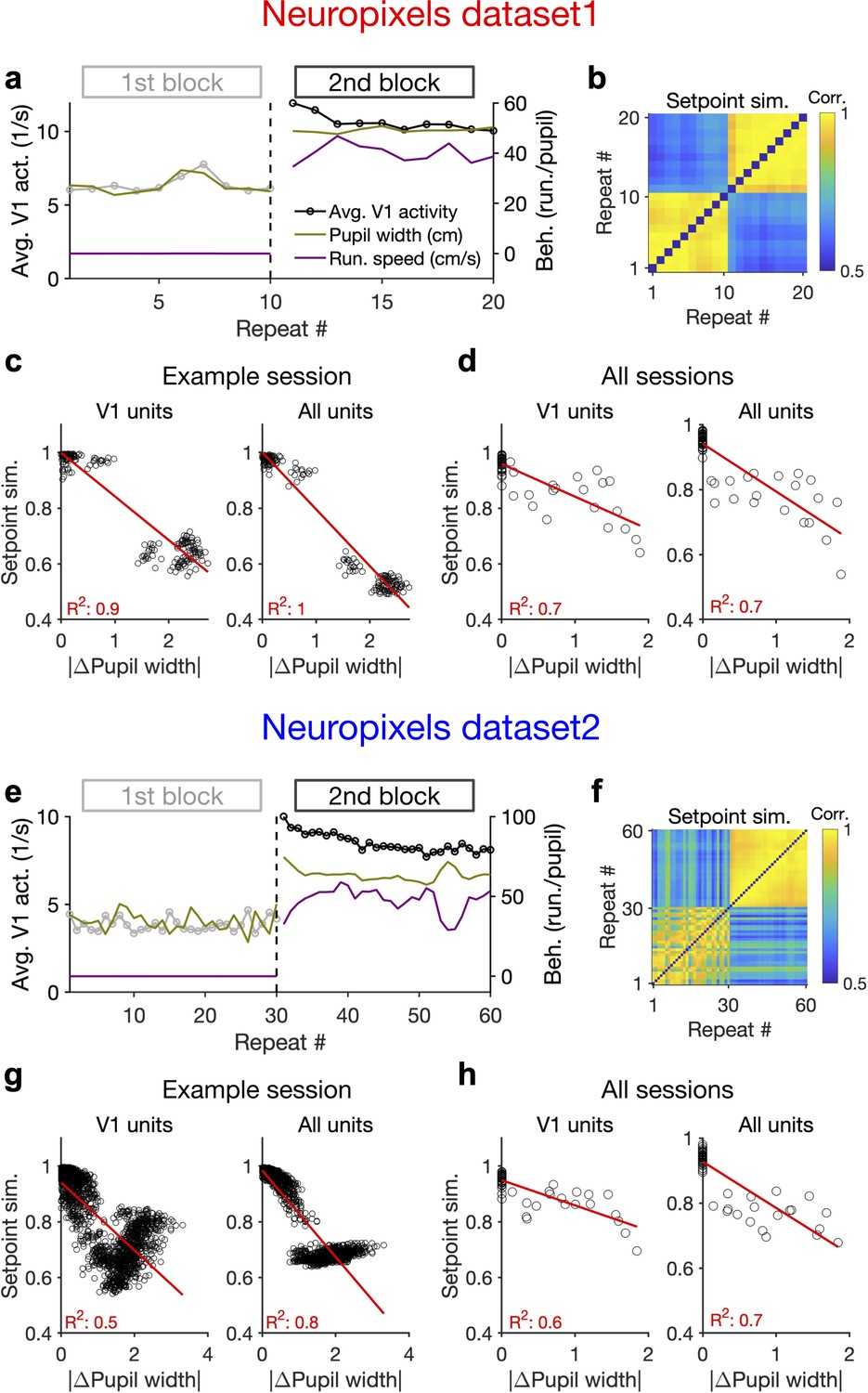
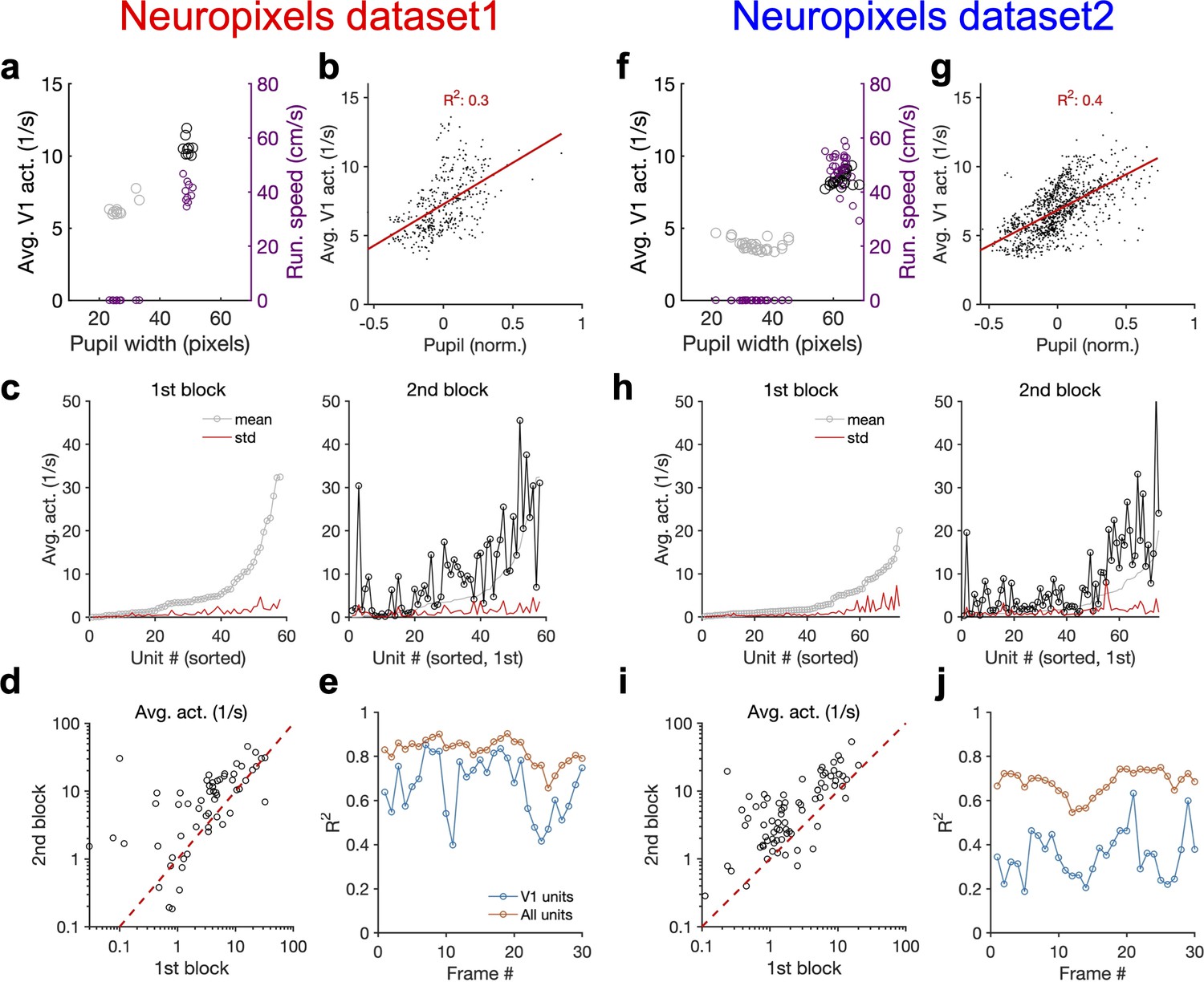
Behaviour modulates the setpoint of responses.
(a), Average population activity and behavioural parameters (pupil size and running speed) during the first and second blocks of presentation of natural movie 1 (same examples sessions as Figure 1). Grey, first block; black, second block; each point corresponding to the average in one repeat of the movie. (b) Setpoint similarity is calculated as the correlation coefficient of population vectors composed of average activity of units during each repeat of movie presentation. Change in the behavioural state (as quantified by the pupil size) between the two blocks is correlated with a drastic decrease in the average between-block setpoint similarity. Note that transient changes of pupil within each block also modulate the setpoint similarity. (c), Setpoint similarity (as in b) as a function of change in pupil size (z-scored pupil width) between the movie repeats, when the population vectors of setpoints are composed of V1 units (left) or all recorded units (right). (d), Dependence of setpoint similarity on pupil change for all sessions, calculated from within-block and across-block averages in each session. (e–h), Same as (a–d) for dataset 2. Source data (for the change in pupil width and setpoint similarity between pairs of movie repeats) are provided for individual sessions across the two datasets (Figure 4—source data 1).
-
Figure 4—source data 1
Related to Figure 4.
Source data (for the change in average z-scored pupil width and setpoint similarity between pairs of movie repeats) for individual sessions across the two Neuropixels datasets.
- https://cdn.elifesciences.org/articles/77907/elife-77907-fig4-data1-v2.xls
Figure 4—figure supplement 1
Average activity of units is modulated by behavioural state.
(a) Average population activity (left y-axis) and running speed (right y-axis) as a function of pupil size, for the example shown in Figure 4a from Neuropixels dataset 1. (b) Average population activity of V1 units during each movie presentation as a function of pupil size from all recorded sessions. Pupil size for each repeat is normalized (within each session) by subtracting the mean value (across repeats) and dividing by it. (c) For the example session in Figure 4, the average (across movie frames) activity of V1 units is calculated and their mean and SD across movie repetitions in each block are shown. Units are sorted in both blocks according to the mean in the first block. (d) Average activity (across movie frames and repeats) of units during the second block versus the first. Note the logarithmic scales. (e) R2 values of the regression fits to the data like Figure 4c, when the population vectors are composed of the average activity of units during presentation of each individual frame (1 s long) of the natural movie. (f–j) Same as (a–e) for Neuropixels dataset 2.
Figure 4—figure supplement 2
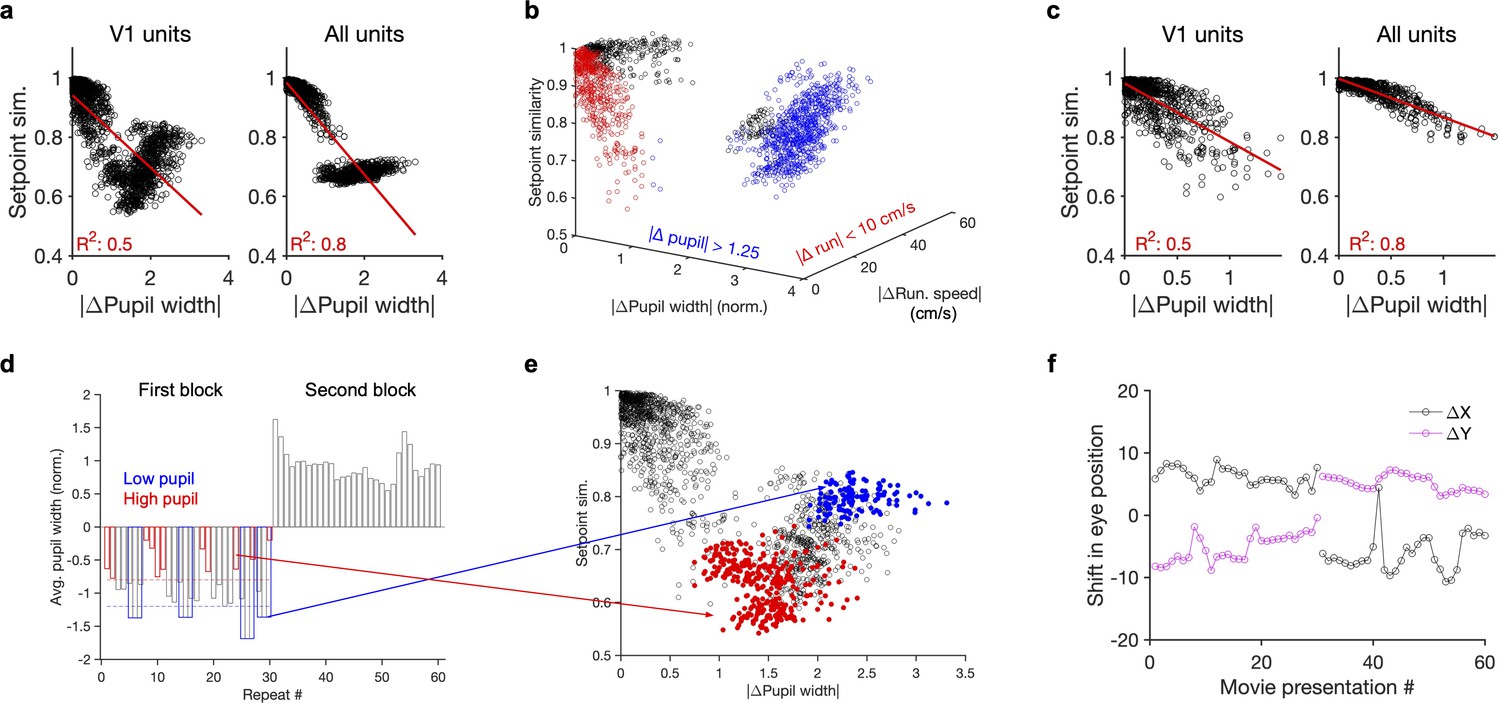
Nonmonotonic relationship between setpoint similarity and behaviour.
(a) Relationship between setpoint similarity and change in pupil size for the same example session as Figure 4g. (b) Same data as (a) when setpoint similarity is plotted as a function of both changes in pupil size and change in running speed between movie repeats. Red data points indicated movie repeats with small difference of average running speed between them ( run. speed <10 cm/s), and blue data points indicate movie repeats with large changes of average pupil width (| pupil width| > 1.25). Black: other data points. (c) Same as (a) for red data points in (b) (for movie repeats with small changes of average running speed between them). (d) Average pupil width (normalized by z-scoring) during each movie presentation in the first (repeat #1–30) and the second (repeat #31–60) blocks of presentations. Red and blue bars show, respectively, the movie presentations above (>–0.8; red dashed line) and below (<–1.2; blue dashed line) the average of the pupil size in the first block. (e) Same as (a) when setpoint similarity between specific pairs of movie repeats are colour coded. For pairs of movie repeats with one in the first block and the other in the second block, setpoint similarity is colour coded according to the average pupil width during the movie repeat in the first block, with red and blue circles corresponding to blue and red bars in (d), respectively. (f), Shift in the eye position across movie presentations. and denote deviation of the average centre of the pupil (X and Y) from their grand average value during the whole session.
Figure 4—figure supplement 3
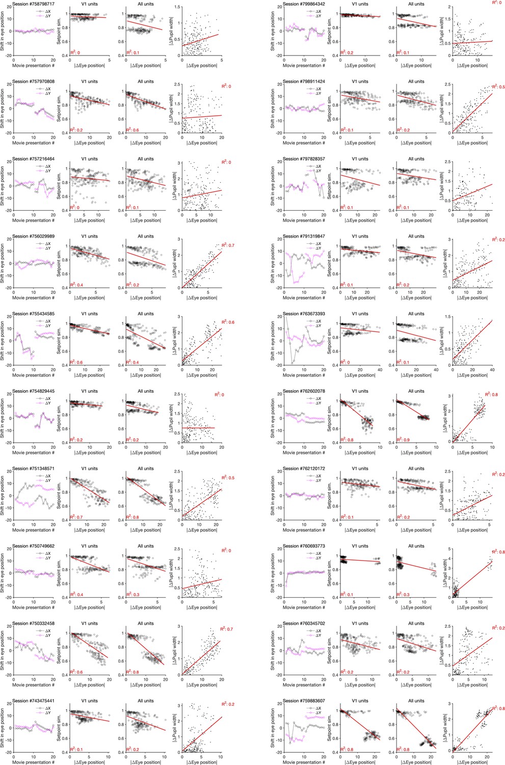
Changes in the pupil centre and their relation to setpoint similarity and changes in pupil width (for sessions in Neuropixels dataset 1).
First column: same as Figure 4—figure supplement 2f, showing shift in the eye position across movie presentations for each session (session # indicated on the top). Second and third columns: same as Figure 4—figure supplement 2a, when setpoint similarity is plotted against changes in the average eye position between movie repeats. Fourth column: relation between changes in eye position and changes in pupil width.
Figure 4—figure supplement 4
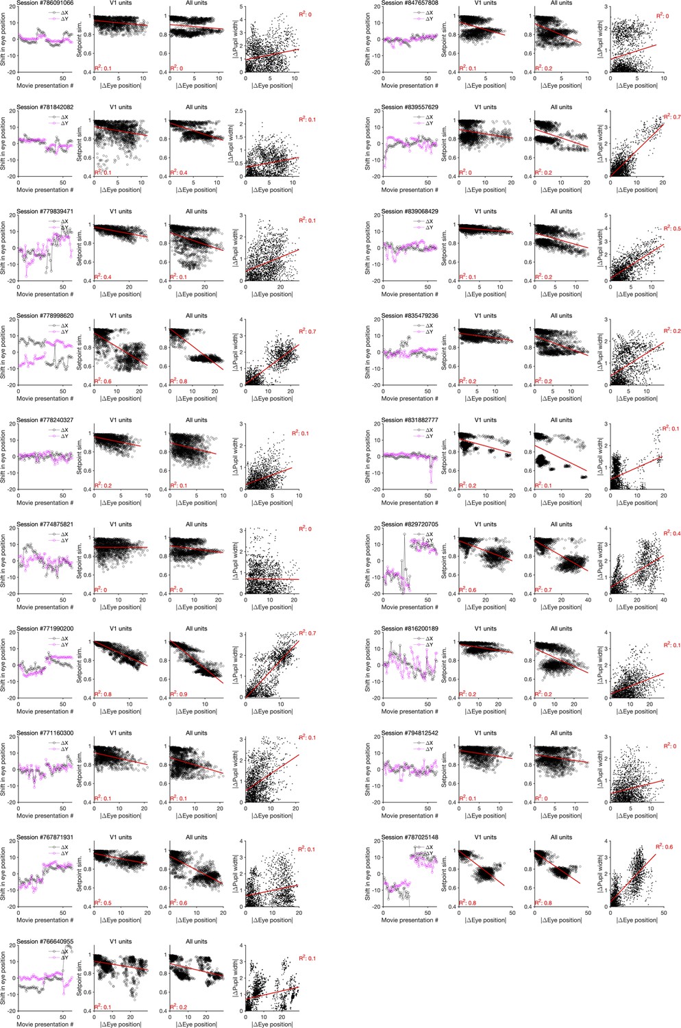
Changes in the pupil centre and their relation to setpoint similarity and changes in pupil width (for sessions in Neuropixels dataset 2).
Same as Figure 4—figure supplement 3 for Neuropixels dataset 2.
Figure 4—figure supplement 5
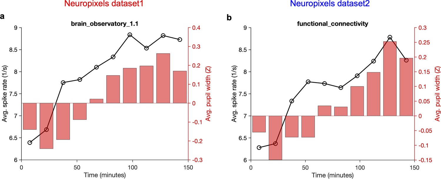
Overall average activity of units and average pupil width gradually increase during the recording session.
Average activity of units (across all recorded units and all sessions/animals) across time during the recording session. Each recording session (~2.5 hr) is broken to 10 time bins and the mean value within that time bin is calculated. The average z-scored value of pupil width (averaged across animals and within the same time bins) is shown on the right (red bars). (a) Neuropixels dataset 1; (b) Neuropixels dataset 2. Note that for both datasets the average activity increases gradually from ~6 spikes/s to ~9 spikes/s at the end (~50% increase). Also, note the similar, gradual increase of pupil width.
Figure 5 with 3 supplements
Behaviour reliably modulates responses during active states.
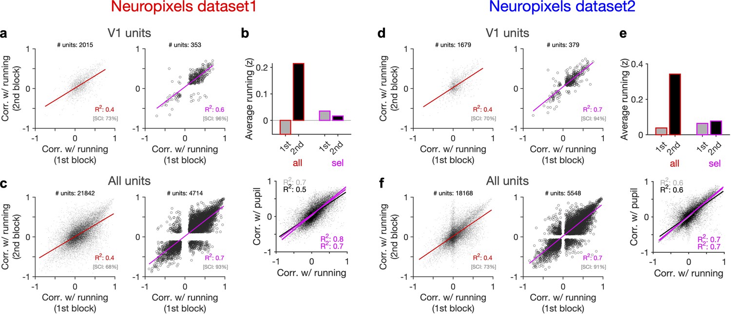
(a) Correlation of activity with running during second block against the first block for all V1 units (left) and for selected sessions and units (right). In the latter case, only sessions with similar average running between the two blocks, and units with significant correlation with running, are selected (see Figure 5—figure supplement 1 and ‘Methods’ for details). In addition to the regression analysis (quantified by the value of R2), a second metric (sign constancy index [SCI]) is also used to quantify the reliability of modulations by behaviour. For each unit, the sign of correlation with running in different blocks is compared and the fraction of units with the same sign is reported as SCI. (b) Upper: average z-scored value of running in the first and second block across all units/sessions (all; red) and for selected ones (sel; magenta). Lower: correlation of all V1 units with pupil size against their correlation with running in first (grey) and second (black) blocks. Magenta: regression fits for selected units/sessions only. (c) Same as (a) for recorded units from all regions. (d–f) Same as (a–c) for dataset 2.
Figure 5—figure supplement 1
Significant modulation of units by behaviour.
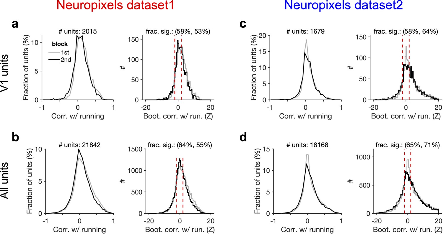
(a) Left: distribution of correlation of V1 units’ activity with running during first and second blocks of presentation of natural movie 1. Right: distribution of bootstrapped correlations with running. Correlation coefficient (CC) of each unit’s activity with 100 randomly shuffled versions of the running speed is calculated. The z-score of bootstrapped correlation (Z) is calculated by subtracting the mean of this distribution from the unshuffled CC and dividing it by the SD of the distribution (see ‘Methods’ for details). Bootstrapped correlations are calculated during the first (grey) and second (black) blocks separately. Significant correlations are taken as units for which |Z| > 2 (indicated by dashed red lines). Fractions of significant correlations during the first and second blocks are indicated on the top, respectively. (b) same as (a) for all recorded units. (c, d) Same as (a, b) for dataset 2.
Figure 5—figure supplement 2
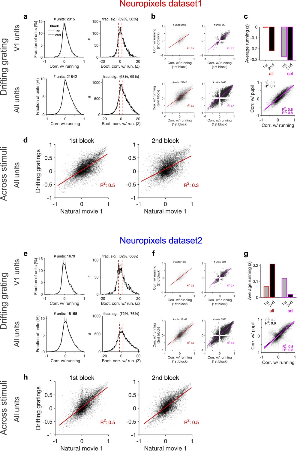
Consistent modulation of neuronal responses by behaviour across blocks of presentation of drifting gratings and across stimuli.
(a) Left: distribution of correlations with running during the first and second blocks of presentation of drifting gratings across all sessions. Right: distribution of the z-score of bootstrapped correlations (Z) with running (see ‘Methods’ and Figure 5—figure supplement 1). Significant correlations with running are defined as |Z| > 0.2. (b) Correlation with running of units during the second block against the first block for all units and sessions (left; red) and for selected units (right; magenta), where sessions with similar levels of running between the two blocks and units with significant correlations are selected. (c) Upper: average running during the first and second blocks for all sessions (all; red) and for selected units (sel; magenta). Lower: correlation of all units with pupil versus their correlation with running during the first (grey) and second (black) blocks. Magenta: regression fits for selected units only. (d) Correlation of all units with running speed during the presentation of drifting gratings versus correlations with running obtained during the presentation of natural movie 1 in the first and second blocks of presentations, respectively. (e–h) Same as (a–d) for dataset 2.
Figure 5—figure supplement 3
Consistent modulation of neuronal responses by behaviour across stimuli, regions, and datasets.
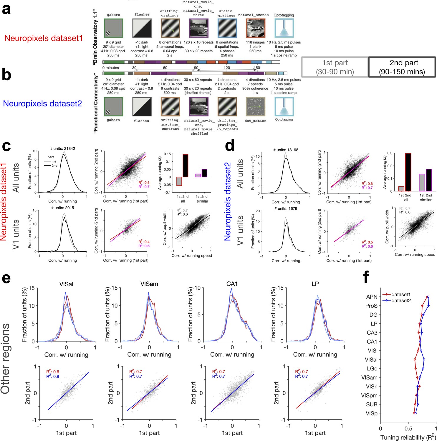
(a, b) Analysis of the reliability of behavioural tuning in two parts of each session in the two datasets. The composition of stimulus sets in each session type is shown, with the type, sequences, and the length of each stimulus presentation indicated. In both datasets, correlation of units with running speed is calculated in two parts: first part from 30 to 90 min, and the second part from 90 to 150 min. (c, d) Similar to Figure 5—figure supplement 2a–c for the first and second parts of the sessions in dataset 1 (c) and dataset 2 (d). (e) Upper: distribution of correlations with running for units recorded from different regions. Results for the two parts of the sessions (lighter lines denoting the first part) and both datasets (red: dataset 1; blue: dataset 2) are overlayed. Sessions where the average running between the two parts are too different are excluded (exclusion criteria: |Z2-Z1| > 0.3, where Z1 and Z2 are the average of the z-scored value of running speed in the first and second parts, respectively). Lower: correlation with running in the second part against the first part in each region for dataset 1 (red) and dataset 2 (blue), respectively. Lines show the best-fitted least-square regression lines, with numbers denoting the R2 values of the fit in each case. (f) Tuning reliability (average R2 values in e) for different regions across the two datasets. Regions key: [visual cortex, VIS] VISp: primary visual cortex; VISl: lateromedial area; VISrl: rostrolateral area; VISal: anterolateral area; VISam: posteromedial area; VISam: anteromedial area. [Hippocampal formation] CA1: cornu ammonis 1; CA3: cornu ammonis 3; DG: dentate gyrus; SUB: subiculum; ProS: prosubiculum. [Thalamus] LGd: lateral geniculate nucleus; LP: lateral posterior nucleus. [Midbrain] APN: anterior pretectal nucleus.
Figure 6
Stimulus dependence of behavioural variability and setpoint similarity.
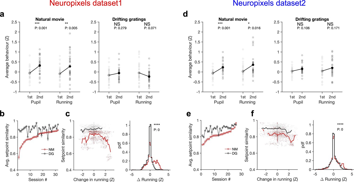
(a) Average pupil size and running speed during the first (grey) and second (black) blocks of presentation of natural movies (left) and drifting gratings (right) for different sessions (empty circles). Filled circles: the mean across sessions. Pupil size and running speed are z-scored across each session, respectively. p-Values on top show the result of two-sample t-tests between the two blocks. NS, p>0.05; *p≤0.05; **p≤0.01; ***p≤0.001; ****p≤0.0001. (b) Average setpoint similarity between the two blocks of presentation of natural movie 1 (NM) and drifting gratings (DG) for different sessions. Sessions are sorted according to their average setpoint similarity for NM. Population vectors are built out of the average responses of all units to 30 randomly chosen frames (1 s long). The correlation coefficient between a pair of population vectors from different blocks (within the same stimulus type) is taken as setpoint similarity. The procedure is repeated for 100 pairs in each session and the average value is plotted. Error bars show the SD across the repeats. (c), Left: setpoint similarity as a function of the difference in average running, , where and are the average running during randomly chosen frames in the first and second block, respectively. The lines show the average of the points in 40 bins from the minimum to the maximum. Right: distribution of changes in running for different stimuli. The probability density function (pdf) is normalized to the interval chosen (0.25). (d–f) Same as (a–c) for dataset 2. Source data (for the average z-scored pupil width and running speed in each block) are provided for individual sessions across the two datasets (Figure 6—source data 1).
-
Figure 6—source data 1
Related to Figure 6.
Source data (for the average z-scored values of pupil width and running speed in each block) for individual sessions across the two Neuropixels datasets.
- https://cdn.elifesciences.org/articles/77907/elife-77907-fig6-data1-v2.xls
Figure 7 with 2 supplements
Decoding generalizability of natural images improves by focusing on reliable units.
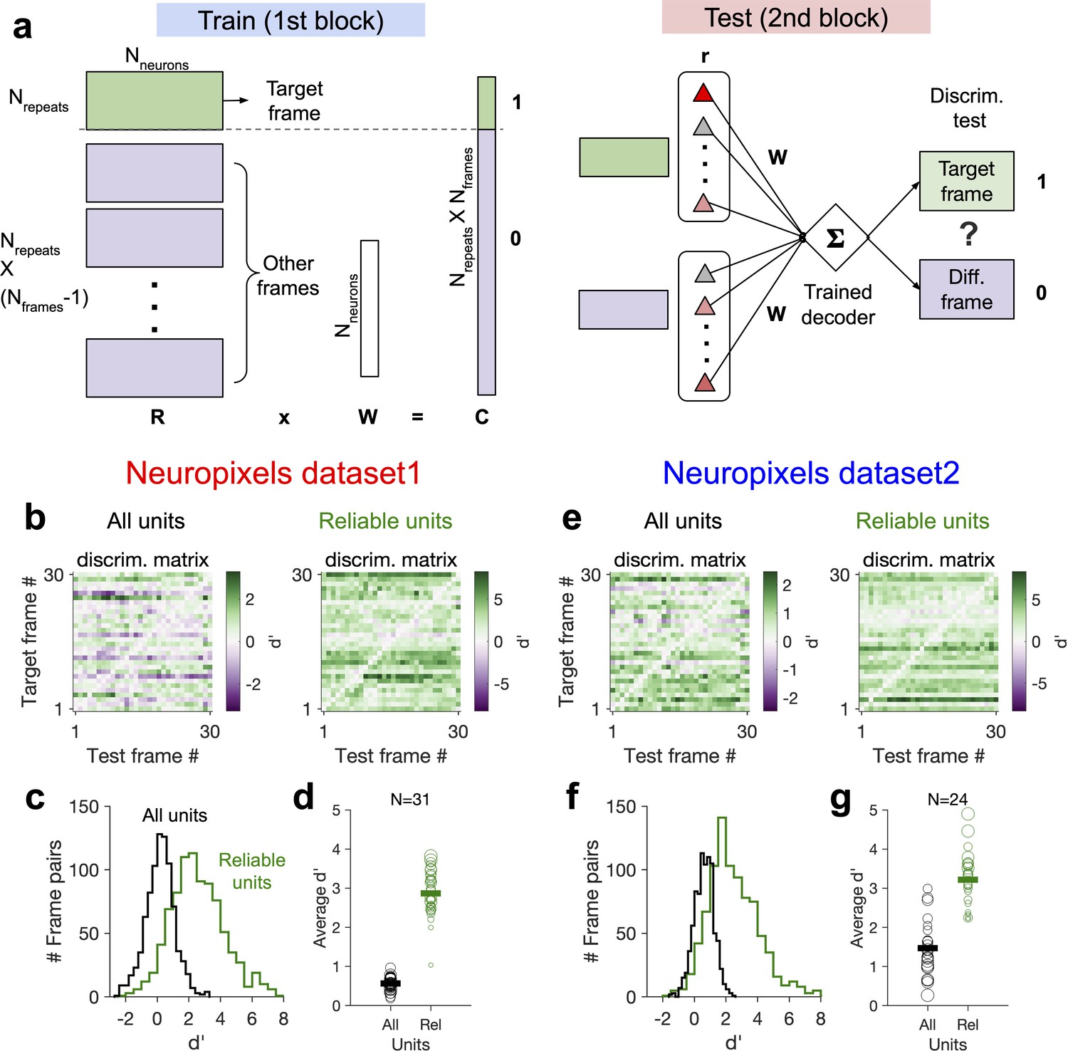
(a) Schematic of a decoder which is trained on the population activity during the first block of presentation of the natural movie (upper) and tested on the second block of presentation to discriminate different frames of natural images from each other (out-of-distribution transfer; see ‘Methods’ for details). (b) Matrix of discriminability index (‘Methods’), d′, between all combinations of movie frames as target and test, when all units (left) or only units with high stimulus reliability (right) are included in training and testing of the decoder. (c) Distribution of d′ from the example discriminability matrices shown in (b) for decoders based on all units (black) and reliable units (green). Reliable units are chosen as units with stimulus reliability (‘Methods’) of more than 0.5. (d) Average d′ for all mice, when all units or only reliable units are included. Size of each circle is proportionate to the number of units available in each session (sessions with >10 reliable units are included). Filled markers: average across mice. (e–g) Same as (b–d) for dataset 2. Data in (b, c) and (e, f) are from the same example sessions shown in Figure 1c and Figure 1f, respectively.
Figure 7—figure supplement 1
Decoding natural images does not improve by focusing on behaviourally modulated units.
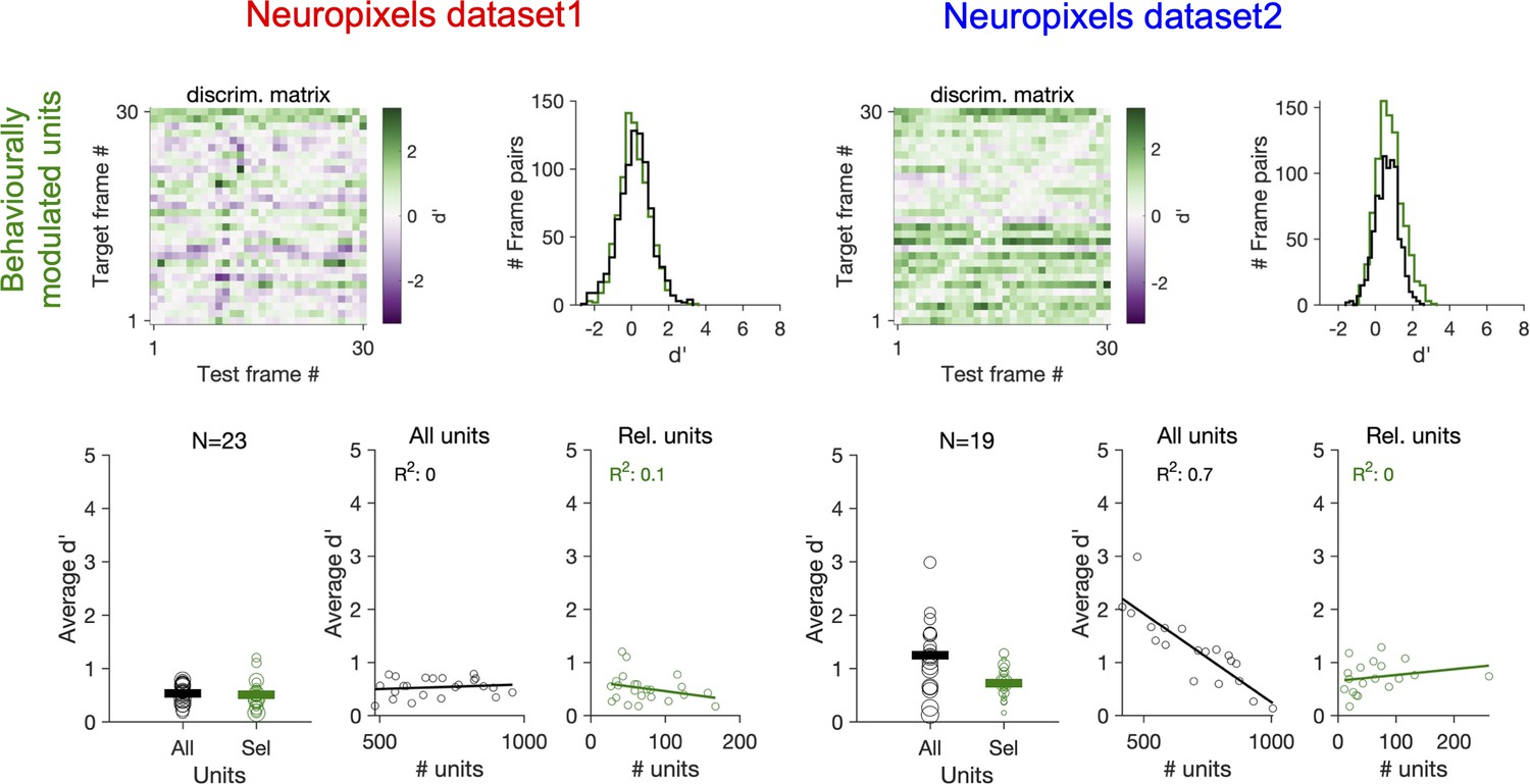
Same as Figure 7c and d when reliable (Rel.) units are chosen as units with strong behavioural modulation (correlation with running speed of more than 0.5), instead of units with strong stimulus reliability (Figure 7). Relation between average d′ and the number of units available for decoding in each session (all units or behaviourally reliable units) is plotted on the bottom.
Figure 7—figure supplement 2
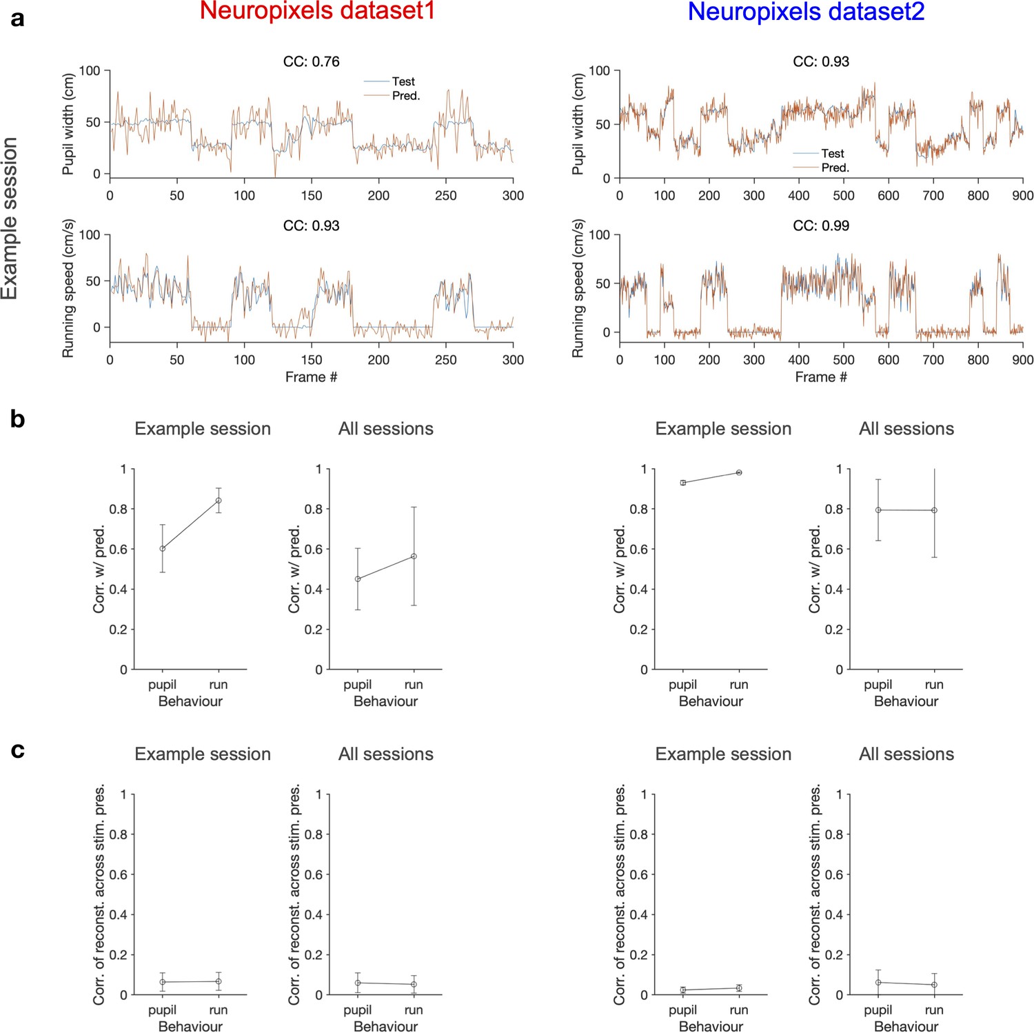
Decoding behavioural states from the population activity.
(a) A linear decoder is trained to predict the pupil width (upper) and the running speed (lower) of the animal from the activity of all recorded units in each session. It is trained on the data from half of randomly chosen movie presentations from both blocks (not shown) and tested on the other half of movie presentations (orange traces). The target values (test) for a specific randomization are shown in blue (note that the order of movie repeats is randomized, while the order of movie frames within each movie presentation is preserved). The quality of prediction is quantified by the correlation coefficient (CC) of test and predicted traces in each case (indicated for the example sessions on top of each behaviour, respectively). Example sessions are the same as in Figure 1 and Figure 7. (b) Average correlation of the predictions with behaviour for multiple repeats of the decoding with different random choices of train and test sets, for the example sessions shown in (a) (100 repeats) and for all sessions (10 repeats per each session). The mean and SD of the correlations across repeats are plotted. (c) The optimal weights obtained from the decoders in (b) are used to weight the neural activity and obtain a readout (similar to predictions in a). The readout activity is then used to assay the stimulus-related content of the behavioural decoder. A matrix of CC of the readout activity between different repeats of the movie is calculated. The average of the off-diagonal entries of the matrix is taken as the correlation of reconstructed activity across multiple stimulus presentations. The mean and SD of this across multiple randomisations (as in b) are plotted in (c) Left: Neuropixels dataset 1; right: Neuropixels dataset 2.
Additional files
-
Supplementary file 1
Information of recording sessions in different datasets.
- https://cdn.elifesciences.org/articles/77907/elife-77907-supp1-v2.docx
-
Transparent reporting form
- https://cdn.elifesciences.org/articles/77907/elife-77907-transrepform1-v2.docx
-
Source code 1
- https://cdn.elifesciences.org/articles/77907/elife-77907-code1-v2.zip
Download links
A two-part list of links to download the article, or parts of the article, in various formats.
Downloads (link to download the article as PDF)
Open citations (links to open the citations from this article in various online reference manager services)
Cite this article (links to download the citations from this article in formats compatible with various reference manager tools)
Contribution of behavioural variability to representational drift
eLife 11:e77907.
https://doi.org/10.7554/eLife.77907


