Cross-modality synthesis of EM time series and live fluorescence imaging
- Molecular Cytology Core, Memorial Sloan Kettering Cancer Center, United States
- Electron Microscopy Facility, University of Lausanne, Switzerland
- Developmental Biology Program, Memorial Sloan Kettering Cancer Center, United States
Figures
Figure 1 with 2 supplements
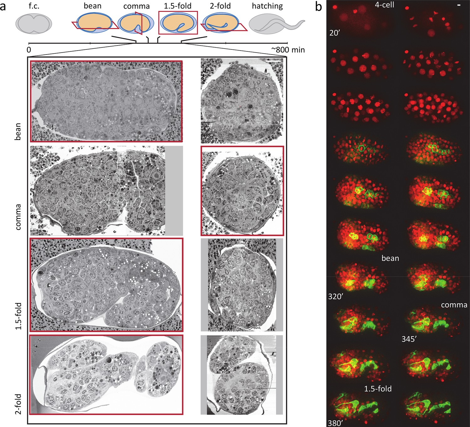
EM and FM time series of C. elegans embryogenesis with complementary spatial and temporal resolution.
All scale bars indicate 5 μm. (a) Overview of EM data and their placement in the time course of C. elegans embryogenesis. Cartoons show body shape and the approximate physical sectioning plane orientation is shown in red. Orthogonal views of each dataset are shown below, with the view corresponding to physical sectioning outlined in red. f.c., first clevage or cell division. (b) An example FM series (see Figure 1—video 1) with a ubiquitous histone marker (red) and a cnd-1 promoter driven membrane marker labeling a subset of neurons (green). Representative time points are shown as max projection. Time stamps are min post first cell division (pfc).
Figure 1—figure supplement 1
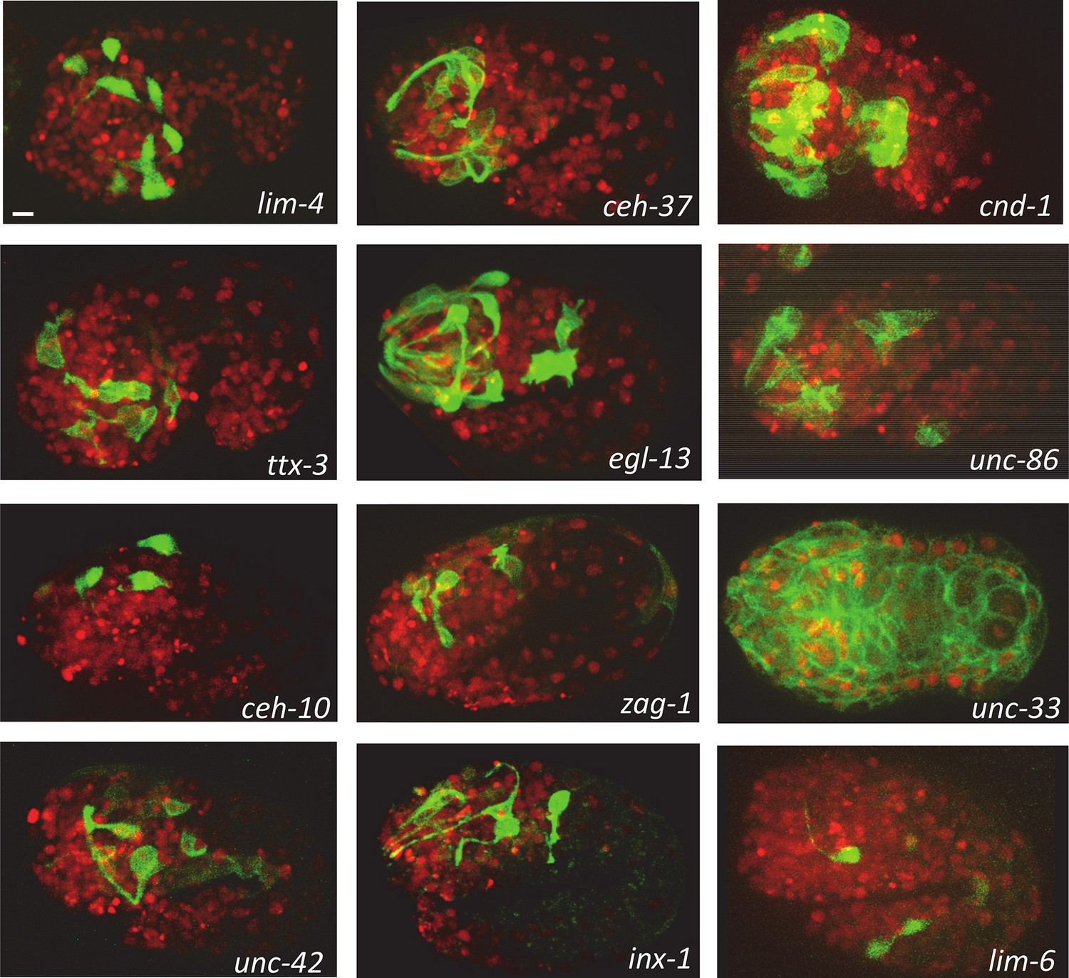
Overview of FM datasets.
Max projection of representative time point for the FM data used. Each strain carries a ubiquitous histone marker (red) and a cell membrane marker (green) driven by a specific promoter (shown in each picture). See also Supplementary file 1d. Scale bar indicates 5 μm.
Figure 1—video 1
FM embryo.
Max projection movie of 8 hours of development of a C. elegans embryo with a ubiquitous histone marker (red) and a cnd-1 promoter -driven membrane marker labeling a subset of neurons (green). Temporal resolution of 1 frame/min. Same embryo as shown in Figure 1.
Figure 2 with 1 supplement
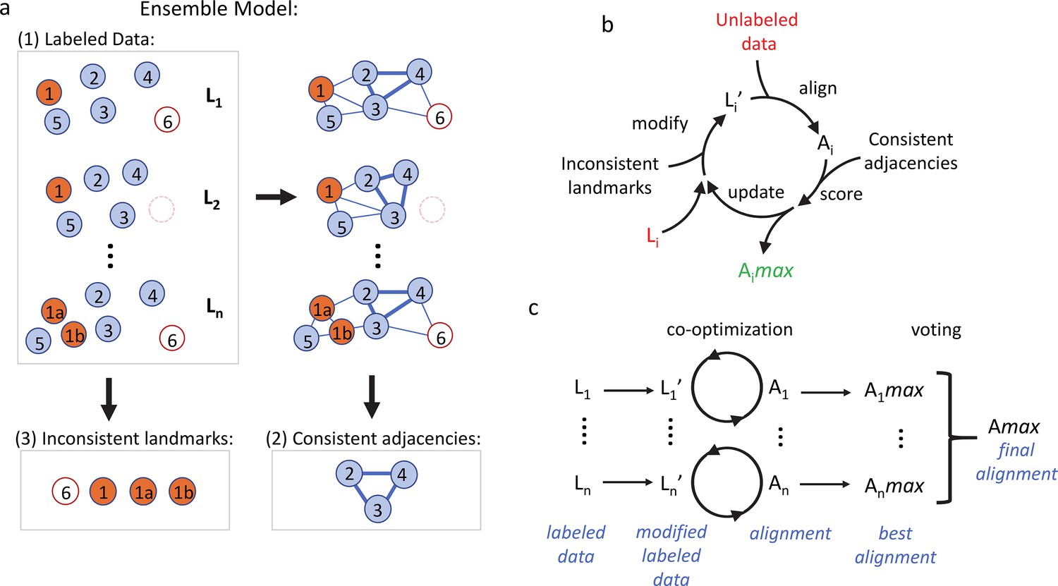
The co-optimization algorithm for cross-modality alignment of developmental data.
(a) Components of the ensemble model. Circles represent landmarks. Numbers in each circle mark the corresponding landmarks across individual labeled data (L1 to Ln). 1a and 1b denote a split of 1 (cell division or other separation of one landmark into two) and the empty circle indicates the disappearance of 6 (cell death or other transient landmark disappearance). Lines represent computed adjacencies, among which thick lines represent consistent adjacencies. (b) Co-optimization of landmark composition in a labeled dataset Li and alignment Ai between Li and unlabeled data. Li is iteratively modified to Li’, aligned, and scored to judge each modification. Modifications that improve score are accumulated to yield an optimized Li’ and corresponding alignment Aimax. (c) The overall process of deriving correlated identities for an unlabeled dataset. Each labeled dataset Li is optimized to generate a best corresponding Aimax. Voting per landmark is then performed over the set of labels across Aimax to achieve a final labeling Amax.
Figure 2—figure supplement 1

Method details.
(a) Pre-alignment Example. Effect of nonlinear pre-alignment. Equivalent nucleus locations in two temporally aligned FM data sets are connected with a tapered cone to show displacement. The top image is these displacements after an optimal affine alignment calculated from all cells. Significant, non-random, displacement between individuals cannot be accounted for by a global affine alignment. The second image shows the same displacements after applying a regularized nonlinear alignment method that does not assume known correspondences GMM-CPD on top of this initial affine alignment. (b) Plot of missing consistent adjacencies for alignments from our approach between the bean EM data and one FM embryo. The labeled data set and expectation model used is set to various temporal offsets from the manually derived optimal temporal alignment. The minimum is centered around the manual alignment, indicating an automated search for an optimally scoring temporal alignment would have produced a similar result. The precise minima is not identical suggesting automation could be used to refine manual alignment guesses. (c) Consistency of identity votes as a quality metric. ROC chart for the fraction of total correct and incorrect identities returned as we accept identities from our alignment of the bean and comma state with fewer votes for the winning identity. This is compared to a ubiquitous alternative quality metric on the same results: distance between matches (computed using one arbitrarily selected FM-labeled data set). For much of its length the votes curve is to the upper left of the distance curve showing it better distinguishes correct and incorrect answers.
Figure 3 with 3 supplements
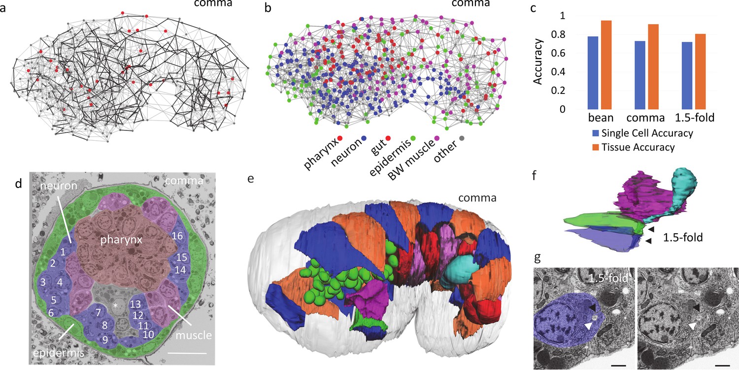
Cross-modality alignment conveys a single-cell view of EM data.
(a) Illustration of the ensemble model for the comma stage. Landmarks (dots) and adjacencies (edges) in a single instance of labeled data. All adjacencies are shown with the consistent adjacencies highlighted in black. Inconsistent landmarks are larger and red. (b) A visualization of the comma stage EM data after alignment. Nucleus centroids are dots colored by major predicted tissue type with color key provided. Adjacencies are shown as gray lines. (c) Accuracy of predicted identities for each EM data at the single-cell and tissue levels. (d) Illustration of EM data annotated by identities. Tissue regions are shaded following the color scheme in b to highlight overall anatomical structure. The excretory canal cell is marked with a star with the nucleus of the excretory duct and part of the pore cell body visible below it. Individual neurons are numbered. Identities as follows are from alignment (-a) or manually confirmed (-c) 1 FLPR/AIZR parent-c, 2 ASER-c, 3 AVBR-c, 4 ASHR-c, 5 AWCR-c, 6 SIBDR-c, 7 AVKR-a, 8 AIYR-a, 9 SMBDR-c, 10 SMBVL-a, 11 AIML-a, 12 AVKL-a, 13 SMDDL-c, 14 FLPL/AIZL parent-a, 15 RMGL-a, 16 ALML/BDUL parent-c. Scale bar indicates 5 μm. (e) 3D reconstruction in comma stage EM data colored to maximize local contrast and showing cell body contours for seam cells (blue and orange), gut cells (alternating shades of red), germ line (cyan), and the excretory canal, duct and pore cells (red, green, and blue respectively) as well as nuclear contours for pharynx (green). (f) 3D reconstruction of the excretory system in the 1.5-fold stage EM data. Red, green, blue and cyan are the excretory canal, duct, pore and gland cell, respectively, as in e. Black arrows point to auto fusion in the duct and pore cell. (g) EM view of lumen (white arrow) and site of auto fusion (black arrow) in the excretory pore cell at 1.5-fold stage. Scale bar indicates 1 μm.
Figure 3—figure supplement 1
Cross-modality alignments.
(a) Illustration of the ensemble model for each EM dataset aligned. See Figure 3a for a detailed explanation. (b) A visualization of all EM data. Nucleus centroids are dots colored by predicted tissue type, matching the color key in panel b. Computed adjacencies are shown as gray edges. (c) Summary of annotations of each EM dataset. A histogram stratified by tissue type for the type of identity available for each cell. Manually verified single cell or tissue type IDs are in blue and red respectively. The identities predicted by our alignment method are gray.
-
Figure 3—figure supplement 1—source data 1
EM annotation bean stage.
Excel spreadsheet containing position and annotation information for bean stage EM.
- https://cdn.elifesciences.org/articles/77918/elife-77918-fig3-figsupp1-data1-v2.zip
-
Figure 3—figure supplement 1—source data 2
EM annotation comma stage.
Excel spreadsheet containing position and annotation information for comma stage EM.
- https://cdn.elifesciences.org/articles/77918/elife-77918-fig3-figsupp1-data2-v2.xlsx
-
Figure 3—figure supplement 1—source data 3
EM annotation 1.5-fold stage.
Excel spreadsheet containing position and annotation information for 1.5-fold stage EM.
- https://cdn.elifesciences.org/articles/77918/elife-77918-fig3-figsupp1-data3-v2.xlsx
Figure 3—figure supplement 2
Consistency and change of adjacency over time.
(a) Adjacency counts from FM data at each stage for cells that are present at all three stages. Ordered by lineage position. Only fully consistent adjacencies (white areas) are used to constrain alignment but quantitative adjacency counts provide a way of characterizing positional variability. Adjacency matrices are available in supplemental data. (b) Change in adjacencies observed between the bean and 1.5-fold stages. Color indicates whether adjacencies have been gained (blue) or lost (red) with darker colors being more consistent. (c) The same matrix as in b, displayed as a graph. Cell node positions are set by a force based layout and edge thickness is proportional to signed adjacency change. Color highlights subgraphs with high internal connectivity, i.e. similar patterns of relative motion, suggesting this representation’s potential wider use in characterizing developmental.
-
Figure 3—figure supplement 2—source data 1
All adjacency information bean stage.
CSV spreadsheets containing the quantitative count of adjacencies found in FM data at bean stage. Spreadsheet contains only entries for consistent landmarks (present at all three stages) to aid comparison between stages. Values vary between 0 for cells that are never adjacent to 39 for cells that are always adjacent (these are used as alignment constraints in our method) significant variation occurs between these values. Complete adjacency information data structures used in alignment are available within.mat data files in source code.
- https://cdn.elifesciences.org/articles/77918/elife-77918-fig3-figsupp2-data1-v2.xlsx
-
Figure 3—figure supplement 2—source data 2
All adjacency information comma stage.
Adjacency information for bean stage, see above for additional details.
- https://cdn.elifesciences.org/articles/77918/elife-77918-fig3-figsupp2-data2-v2.zip
-
Figure 3—figure supplement 2—source data 3
All adjacency information 1.5-fold stage.
Adjacency information for 1.5-fold stage, see above for additional details.
- https://cdn.elifesciences.org/articles/77918/elife-77918-fig3-figsupp2-data3-v2.zip
Figure 3—video 1
3D rendering of embryo landmarks.
Visualization of one example set of embryonic landmarks over time. Lineages with a majority fate for a given tissue type are colored to match tissue color code in Figure 3.
Figure 4 with 2 supplements
Spatial and temporal organization of neuropil formation.
All scale bars 1 μm. (a) FM cross section of a comma stage embryo with a ubiquitous histone marker (red) and a broadly expressed cell membrane label (green) (Barnes et al., 2020). Anterior view. Dotted line encircles the NR and routing of sublateral neurons into the ring. (b) Comparison of resolution in resolving NR in FM and EM. Two images of two-color FM image of developing neurites (red, green, and blue are labeled by the promoters of cnd-1, ceh-10, and zag-1, respectively). Neurite bundles are numbered anterior to posterior. EM showing the corresponding neurites and their placement in the ring at the comma stage. Neurites are labeled with names and colors of the corresponding bundle in FM. (c) Schematic of the NR (anterior view) showing first outgrowths, entry points, and approximate extent of neurites at bean and comma stages. Ovals represent neuronal soma and arrowheads the leading edge. Two arrowheads are shown for the amphid (dark blue) and sublateral (light blue). The earlier arrowhead indicates initial outgrowth, and the latter line and arrow indicates the entry points and approximate outgrowth extent at the bean stage. Moving dorsal to ventral, dorsal outgrowth is green, supralateral red, lateral orange, and ventral purple. See Figure 4—figure supplements 1 and 2 for corresponding EM. Open arrows and associated letters indicate the figure panels that show the location pointed to. (d) EM at comma stage showing the first outgrowth at the supralateral entry point with cells shaded red and named. (e) Comparison of initial outgrowth timing derived from FM and EM. Each dot represents a single neuron or small cluster of neurons. Dot color corresponds to membership in groups as pictured in panel c. Cells that do not clearly correspond to these major entry points are gray (See Supplementary file 1d for details). (f) Number of neurites visible in the cross sections of the ring in panel g. The location of this cross section is indicated by arrow b in panel c. Black arrow indicates bean stage. (g) Axial NR cross sections (neurites shaded cyan) near the lateral midline entry point (the location indicated by arrow g in panel c). (h) Precision in neurite outgrowth dynamics. A resliced view of the dorsal midline at comma stage shows the point left and right sublateral early neurites meet (white arrow). Colors match schematic in c.
Figure 4—figure supplement 1

Earliest neurite outgrowths.
All scale bars 1 μm. (a) Illustration of cell groups at bean stage and approximate extent as in Figure 4c. (b–c) EM image of each outgrowth location with cell areas shaded to match cartoon, also pictured without shading. End of neurite or end of cell body from which the neurite is growing is indicated with an arrow.
Figure 4—figure supplement 2
Early neurites at the comma stage.
All scale bars 1 μm. (a) Illustration of cell groups at comma stage and approximate extent as in Figure 4c. (b–g) EM image of each location with cell areas shaded to match cartoon. Also pictured without shading. End of neurite or end of cell body from which the neurite is growing is indicated with an arrow. In e this also indicates the point where amphid cells pause in their outgrowth.
Figure 5 with 2 supplements
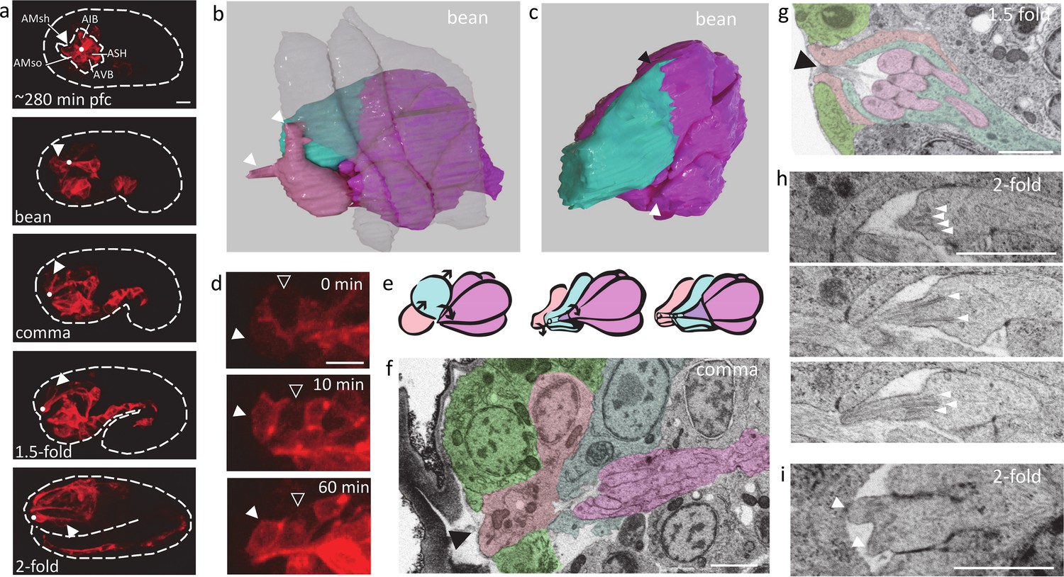
Cell-cell interactions and ultrastructure during amphid organogenesis.
All scale bars 1 μm. (a) FM view of amphid dendrite development with a cnd-1 promoter driven membrane label. Dashed line shows embryo contour. Dot indicates the location of dendrite tips, and arrow the socket and sheath cells. Dashed circle inside the embryo outlines the initial amphid rosette at ~280 min pfc. (b) 3D reconstruction of cells participating in the collective dendrite extension from bean stage EM. Epidermis: semi-transparent; amphid neurons: magenta; sheath cell: cyan; socket cell: pink. Arrows indicate protrusions on the socket cell. (c) The same reconstruction as in b with socket and epidermal cells removed. Black arrow highlights protrusion on the sheath cell. White arrow indicates focal point of amphid neuron protrusions. See also Figure 5—figure supplement 1a-c. (d) Partial max projection of FM image with a cnd-1 promoter driven membrane label showing socket cell (filled arrow) and more weakly labeled sheath cell (open arrow) posterior migration. (e) Schematic of the time course of sensory opening formation. Arrows indicate motion of cells. Colors match b. (f) Resliced view of EM at comma stage highlighting socket cell (tinted rose) shape and relative position to epidermal cells (green), sheath cell (cyan), and dendrites (magenta). Black arrow indicates contact between the socket cell and the exterior of the embryo. (g) EM at the 1.5-fold stage showing the sensory opening. Colors follow f. Arrow indicates the opening to the exterior of the embryo. (h) EM at twofold stage showing three sections of a dendrite tip. White arrows mark nine individual microtubule structures. (i) EM at twofold stage showing a bifurcated dendrite tip, each tip marked with an arrow.
Figure 5—figure supplement 1

Amphid organogenesis.
All scale bars 1 μm. (a) Cross section of dendrite tips at bean stage. Amphids and support cells are labeled and tinted in varying tones to allow individual cells to be distinguished. Confirmed cell identities are shown for all cells visible in cross-section. (b) Exploded diagram rendering of amphids and support cells based on 3D reconstruction. The details of amphid proto-dendrite protrusions are visible. (c) Rendering of same 3D reconstruction of the amphids viewed from an anterior angle highlighting the shared focus of protrusions (indicated by white arrow). (d) Montage of max projection of socket cell over three successive frames in the same cnd-1 promoter-labeled embryo as Figure 5d. Soma marked with a star and protrusion with an arrow. The dynamic events in the socket are visible as it is spatially isolated from the highly expressing nearby amphid dendrites and visible over the more weakly expressing adjacent sheath cell. Dynamic fluctuation is visible throughout the socket cell at this time period (see Figure 5—video 1). (e) Twofold stage dendrite tip. Colors match Figure 5f and g. (f) Dendrite tips showing centrosomes absent at bean stage and present (indicated by arrows) at the comma and 1.5-fold stages.
Figure 5—video 1
Socket, sheath cell migration.
Selective max projection movie of socket and sheath cell migration in C. elegans embryo with cnd-1 -driven membrane label. Same embryo as shown in Figure 5d. A slightly looser cropping is chosen for enhanced context.
Additional files
-
Supplementary file 1
Additional summary tables detailing EM imaging conditions, EM and FM landmark properties, alignment accuracy, strains used in FM imaging, annotation extent and landmarks used to initialize alignment.
- https://cdn.elifesciences.org/articles/77918/elife-77918-supp1-v2.docx
-
Transparent reporting form
- https://cdn.elifesciences.org/articles/77918/elife-77918-transrepform1-v2.docx
Download links
A two-part list of links to download the article, or parts of the article, in various formats.
Downloads (link to download the article as PDF)
Open citations (links to open the citations from this article in various online reference manager services)
Cite this article (links to download the citations from this article in formats compatible with various reference manager tools)
Cross-modality synthesis of EM time series and live fluorescence imaging
eLife 11:e77918.
https://doi.org/10.7554/eLife.77918


