A hardware system for real-time decoding of in vivo calcium imaging data
- Department of Electrical and Computer Engineering, University of California, Los Angeles, United States
- Department of Psychology, University of California, Los Angeles, United States
- David Geffen School of Medicine, University of California, Los Angeles, United States
- Department of Neurology, David Geffen School of Medicine, University of California, Los Angeles, United States
- Integrative Center for Learning and Memory, University of California, Los Angeles, United States
Figures
Figure 1
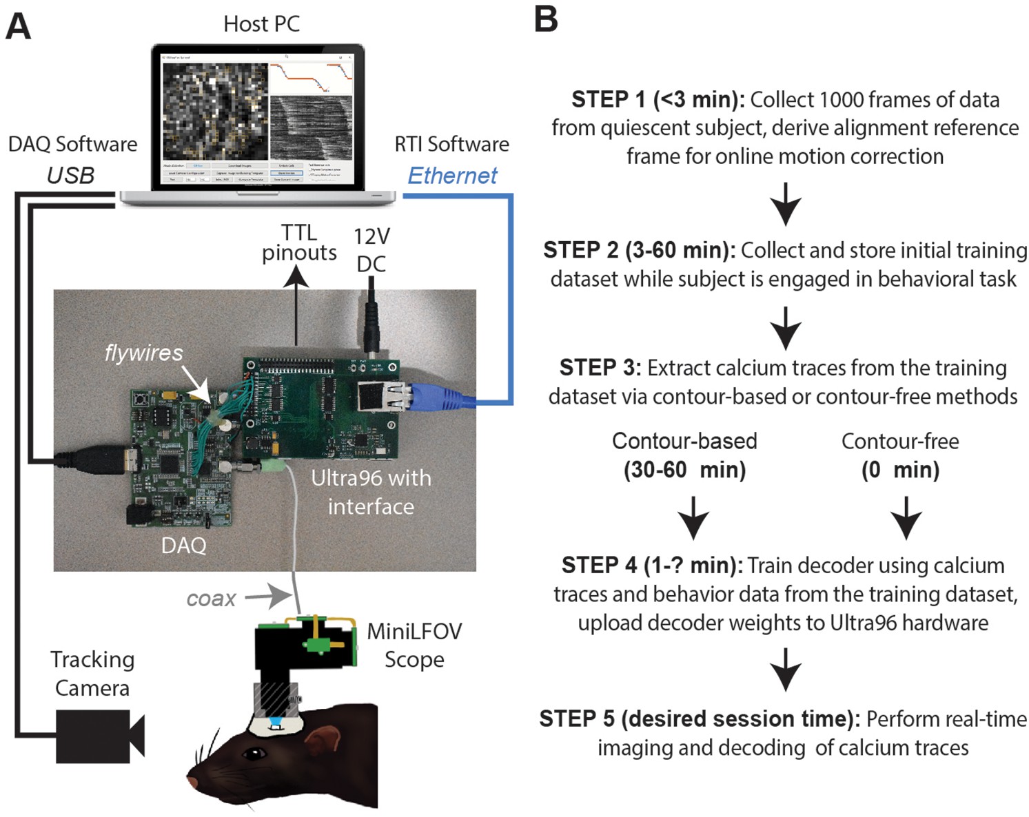
Real-time imaging protocol and system hardware.
(A) Sequence of steps for a real-time imaging and decoding session. (B) Miniscope connects to DAQ via coax cable, DAQ connects to Ultra96 via flywires, host PC connects to Ultra96 via Ethernet and to DAQ via USB 3.0; TTL pinouts from Ultra96 can drive closed-loop feedback stimulation from external devices.
Figure 2
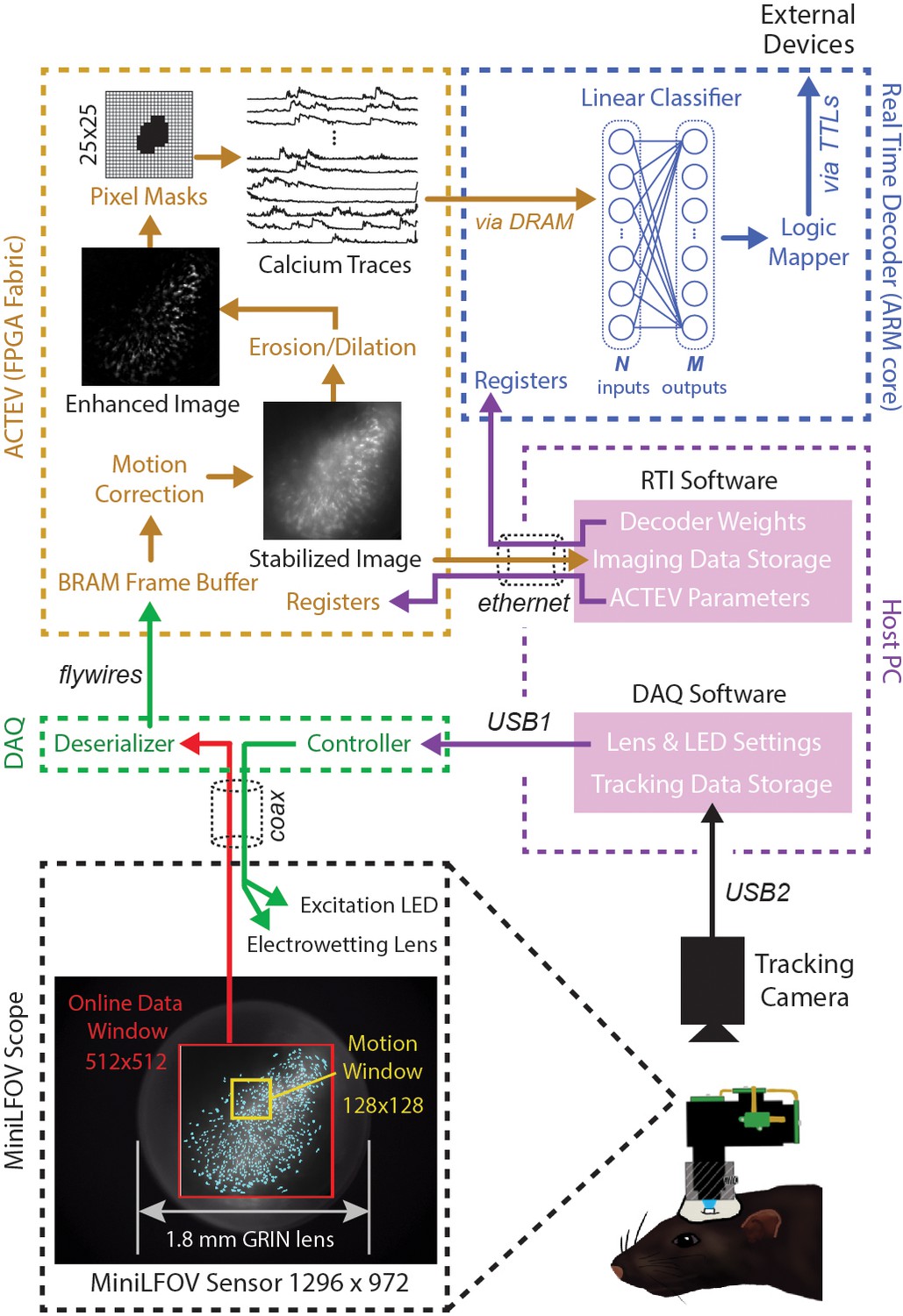
Online imaging and control pipelines.
Serialized video data from the MiniLFOV are transmitted through a coaxial tether cable to the DAQ, where it is deserialized and transmitted via the flywire bus to ACTEV (Accelerator for Calcium Trace Extraction from Video) firmware programmed on the field-programmable gate array (FPGA) of the Ultra96. ACTEV crops the incoming image from its original size (1296 × 972 for the LFOV sensor shown here) down to a 512 × 512 subwindow (manually selected to contain the richest area of fluorescing neurons in each animal) before storing video frames to a BRAM buffer on the FPGA. Subsequent motion correction and calcium trace extraction steps are performed by the FPGA fabric as described in the main text. Extracted calcium traces are stored to DRAM from which they can be read as inputs to a decoder algorithm running on the Ultra96 ARM core. Decoder output is fed to a logic mapper that can trigger TTL output signals from the Ultra96, which in turn can control external devices for generating closed-loop feedback.
Figure 3 with 1 supplement
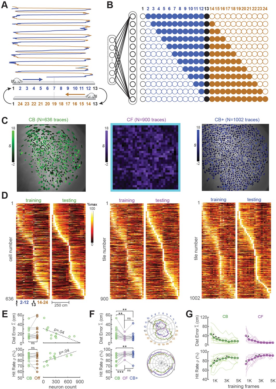
Position decoding from CA1 cells.
(A) The CA1 layer of the hippocampus was imaged while rats ran laps on a 250-cm linear track; for position decoding, the rat’s path was circularized and subdivided into 24 position bins, each ~20 cm wide. (B) N linear classifer inputs (one per calcium trace) were mapped to 12 outputs using a Gray code representing the 24 track positions (open/filled circles show units with target outputs of −1/+1 at each position). (C) Regions of interest (ROIs) from which contour-based (CB, left), contour-free (CF, middle), and expanded contour-based (CB+) calcium traces were extracted in Rat #6; ROI shading intensity shows the similarity score, S, for traces extracted from the ROI. (D) Tuning curve heatmaps from training and testing epochs for CB (left), CF (middle), and CB+ traces extracted from Rat #6; rows are sorted by location of peak activity in the testing epoch. (E) Decoding performance did not differ for CB versus offline (Off) traces (left graphs), but was significantly better for sessions with larger numbers of calcium traces (right graphs). (F) Decoding performance averaged over track positions within each session (left graphs) and over sessions at each circularized track position (right graphs). (G) Decoding performance as a function of training set size; asterisks mark significant improvement with the addition of 500 more frames to the training set. For all panels: *p < 0.05, **p < 0.01, ***p < 0.001.
Figure 3—figure supplement 1
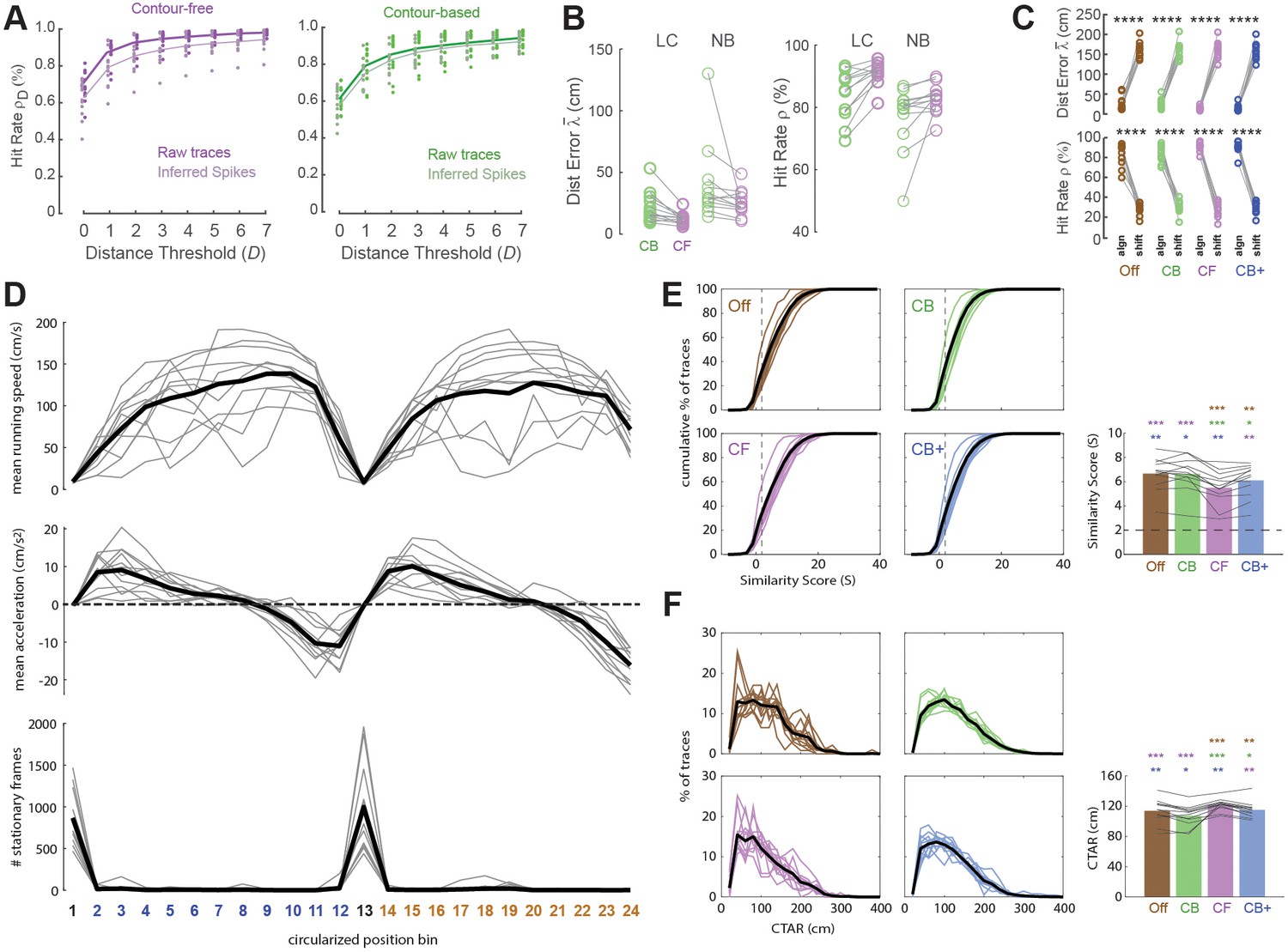
Decoding position from calcium traces on the linear track.
(A) For contour-free (left) and contour-based (right) trace extraction methods, hit-rate accuracy (±D, y-axis) of position decoding was higher when classifier was trained and tested on raw calcium trace values than inferred spike events; ±D is the percentage of predicted position bins falling within a radius of ±D of true position bin. (B) Performance comparison between linear classifier (LC, same as Figure 3F) versus naive Bayes (NB) decoder; NB performs poorly and was thus not implemented for real-time decoding of calcium traces. (C) Decoder predictions are far more accurate after training on 3K frames of calcium traces aligned with position data (‘align’) than circularly shifted against position data (‘shift’). (D) Graphs plot each rat’s mean running speed (top graph), mean acceleration (middle graph), and total number of image frames during which the rat was sitting still (running speed <5 cm/s) in each of the 24 position bins (x-axis for all three graphs); black lines show averages over all rats in each graph. (E) Colored lines plot cumulative distributions of tuning curve similarity scores (S) for offline (Off), contour-based (CB), contour-free (CF), and expanded contour-based (CB+) calcium traces in each rat. The tuning curve similarity score (S) was computed for each trace as S = −log10(P) × sign(R), where R is the correlation between the trace’s tuning curves from the training versus testing epochs, and P is the significance level for R; the p < 0.01 level for the similarity score is S > 2 (dashed lines in each graph) since log10(0.01) = 2. Bar graph (lower right) shows mean S scores for individual rats (black lines) and averaged over rats (colored bars). The mean value of S over sets of traces imaged in each rat was significantly greater than 2 for every rat, indicating that on average calcium traces in CA1 exhibited stable spatial tuning between the training and testing epochs, as required for accurate decoding. A one-way repeated measures analysis of variance (ANOVA) found that the mean S value differed significantly by trace type (F3,44 = 16.2, p < 0.00001); colored asterisks over each bar show significance of an uncorrected paired t-test comparison between that bar versus bar matching the color of the asterisk. (F) Colored lines plot distributions of calcium trace activity ranges (CTARs) for all traces from each rat; CTAR is defined as the total distance (in cm) over which a calcium trace’s tuning curve exceeds 67% of the tuning curve’s peak value. Bar graph (lower right) shows mean CTAR per rat (black lines) and averaged over rats (colored bars). A one-way repeated measures ANOVA found that the mean CTAR value differed significantly by trace type (F3,44 = 9.1, p < 0.001); colored asterisks over each bar show significance of an uncorrected paired t-test comparison between that bar versus bar matching the color of the asterisk. *p < 0.05; **p < 0.01; ***p < 0.001; ****p < 0.0001.
Figure 4
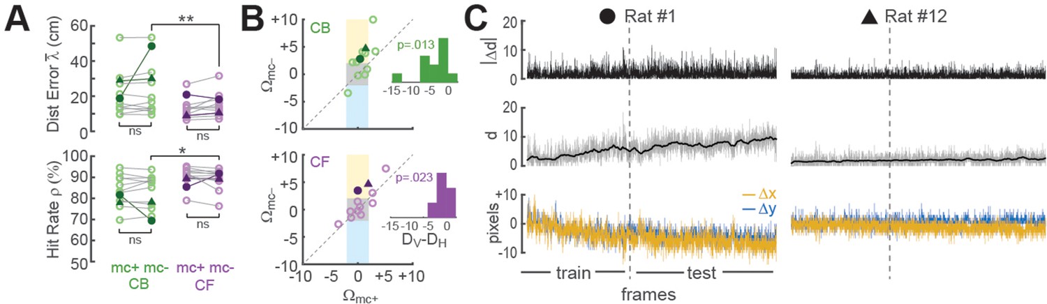
Improvement of place cell decoding by online motion correction.
(A) Session-averaged performance of decoding from CB and CF traces is compared with (mc+) versus without (mc−) online motion correction; filled symbols ‘●’ and ‘▲’ mark data from example sessions shown in panel ‘C’. (B) Scatter plots compare motion artifact scores with (Wmc+) versus without (Wmc−) online motion correction (see main text for explanation of shaded regions); insets show that points lie significantly nearer to the vertical (DV) than horizontal (DH) midline indicating a significant benefit of online motion correction. (C) Displacement of sensor image against reference alignment plotted over all frames in the session (x-axis) for Rat #1 (‘●’) which accumulated a large (~10 pixels) shift alignment error over the session, and Rat #12 (‘▲’) which exhibited transient jitter error but did not accumulate a large shift error; bottom graphs show signed horizontal (Δx) and vertical (Δy) displacement from the reference alignment, middle graphs show distance (d) from reference alignment. And top graphs show absolute value of time derivative of distance (|Δd|) from the reference alignment. *p<.05; **p<.01.
Figure 5
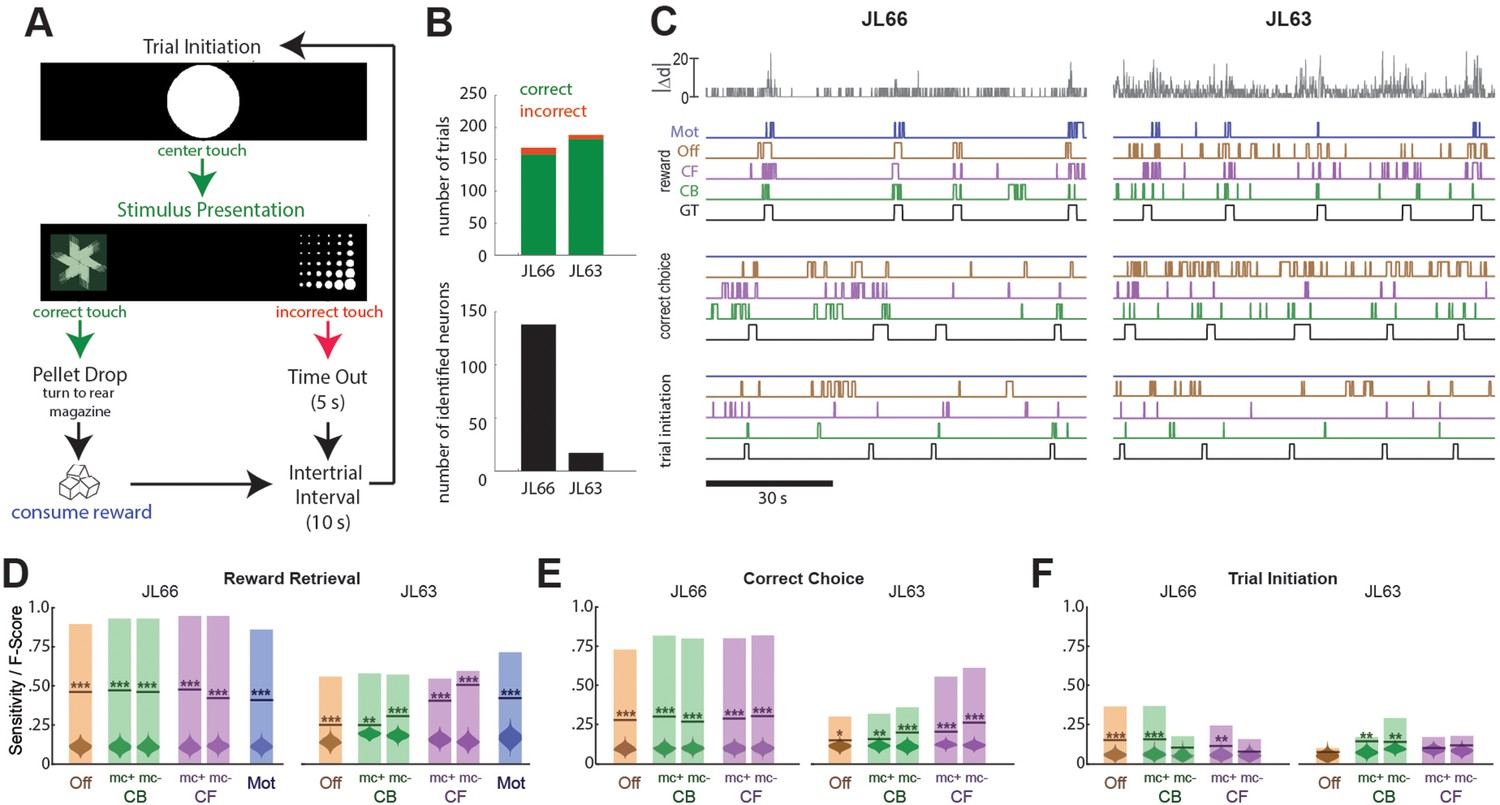
Decoding instrumental behavior from orbitofrontal cortex (OFC) calcium activity.
(A) OFC neurons were imaged while rats performed a 2-choice touchscreen task (see main text). (B) Number of trials (top) and number of neurons identified by constrained non-negative matrix factorization (CNMF) (bottom) during the two analyzed sessions (JL66 and JL63). (C) Jitter error |Δd| (gray traces, top) and real-time predictions of behavior labels (reward retrieval, correct choice, trial initiation) are shown for 90-s periods from the testing epoch of each rat (JL66 and JL63) after the binary tree decoder had been trained on 100 trials of offline (Off), contour-based (CB), or contour-free (CF) calcium traces; black traces show ground truth (GT) behavior labels, blue traces show predictions derived from motion vectors only (Mot). Sensitivity (shaded bars) and F-scores (horizontal lines) are shown for binary classification of reward retrieval (D), correct choice (E), and trial initiation (F) events using decoders trained on Off, CB, CF, or Mot predictors; for online CB and CF predictors, classifer performance is plotted separately for traces derived with versus without motion correction (mc+ vs. mc−), respectively. Violin plot inside each bar shows distribution of F-scores obtained from 1000 shuffles of event labels; asterisks over actual F-scores indicate significant difference from the shuffle distribution (***p < 0.001, **p < 0.01, *p < 0.05).
Figure 6
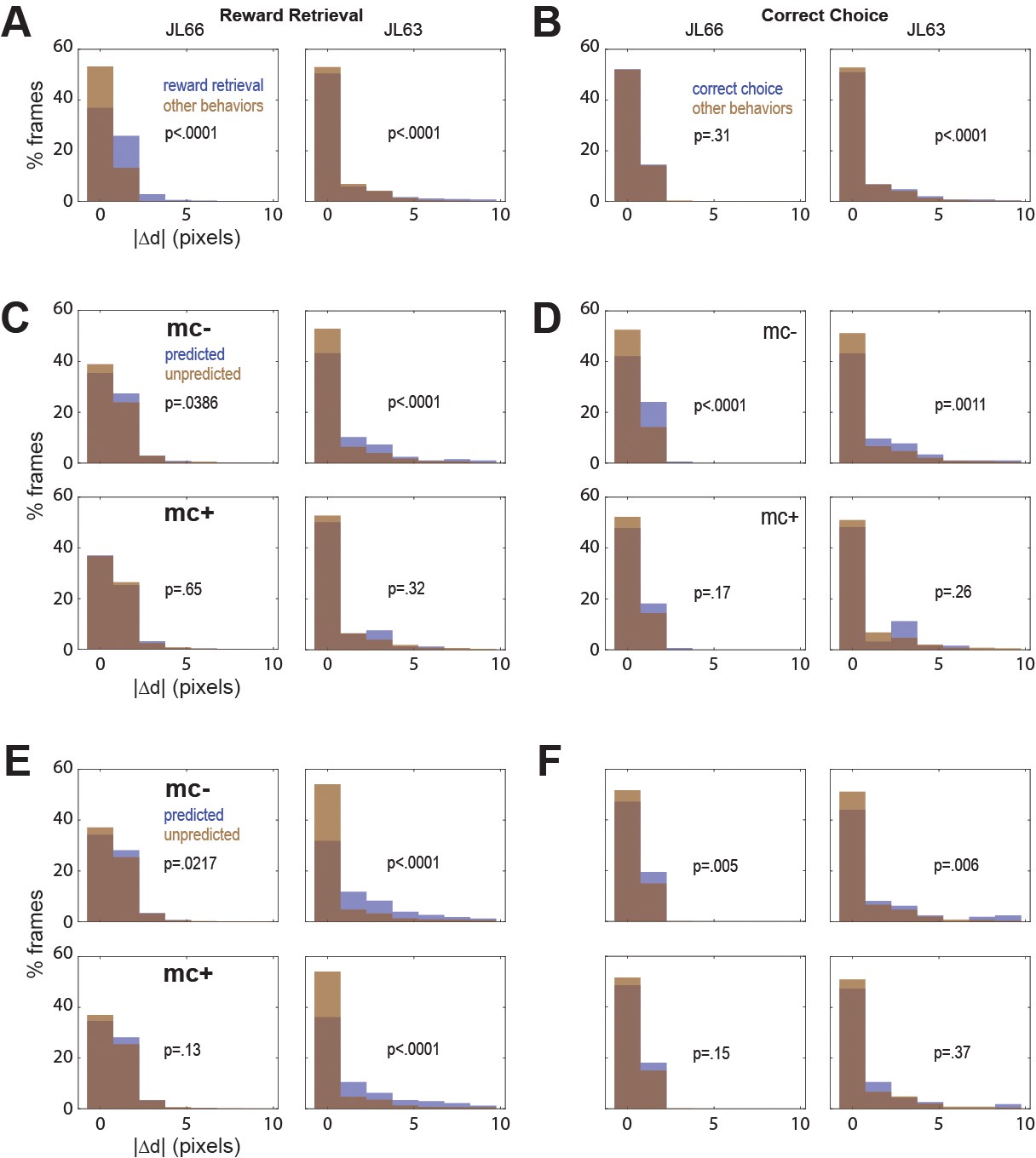
Correlation between motion artifact and decoding accuracy.
(A) Jitter error |Δd| is significantly greater during reward retrieval events than other behaviors in both rats. (B) |Δd| is significantly greater during correct choice events than other behaviors in rat J63 but not JL66. (C) When CB traces are extracted without online motion correction (mc−; top), |Δd| is significantly greater during accurately classified (’predicted’) reward retrieval event frames than inaccurately rejected (’unpredicted’) reward event frames; this difference is abolished when online motion correction is applied before trace extraction (mc+; bottom). (D) Same as ‘C’ but for predictions of correct choice events. (E) Same as ‘C’ but forCF rather than CB traces; note that for rat JL63 online motion correction does not abolish the correlation between decoding accuracy and motion artifact. (F) Same as ‘D’ but for CF traces extracted without (top) versus with (bottom) online motion correction.
Figure 7
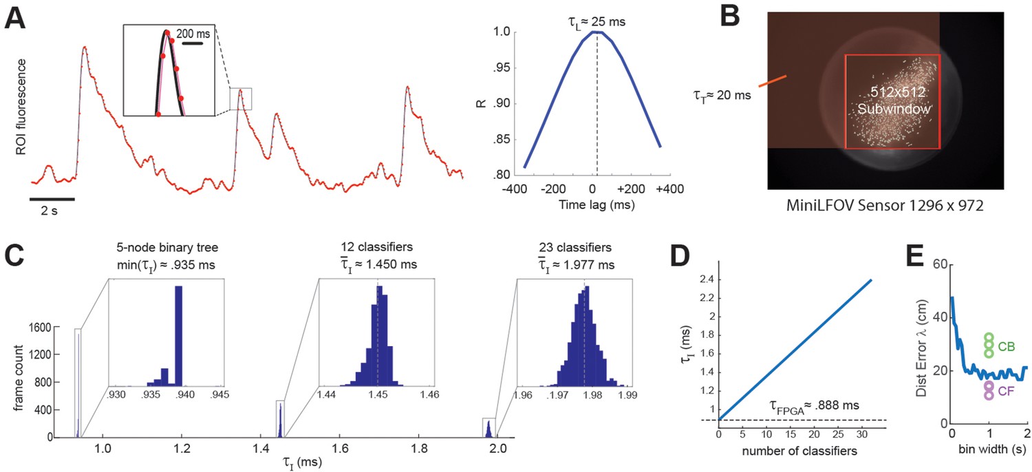
Real-time decoding latency.
(A) Left graph illustrates how the light-gathering delay (τL) is incurred as the sensor time integrates the true fluorescence signal (black line) by summing light gathered during each frame exposure, yielding a time series of binned fluorescence values (red dots) that are delayed from the original fluorescence signal by 1/2 the frame interval (50-ms frame interval was used for this example); right graph shows temporal cross correlogram between the source versus binned fluorescence signals, peaking at 1/2 the frame interval (τL = 25 ms). (B) Transmission delay (τT) is proportional to the number of pixels, P, in the shaded red rectangular area between the upper left corner of the sensor image and the lower right corner of the 512 × 512 imaging subwindow. (C) Image processing delay (τI) for 1204 calcium traces (maximum supported) is proportional to the number of units in the linear classifier’s output layer; empirical distributions of τI are shown for linear classifiers with a single output unit (here τI is approximated as the minimum latency for a 5-node binary tree decoder), 12 output units, and 23 output units. (D) Linear fit to mean τI (y-axis) as function of the number of linear classifiers (x-axis); the y-intercept corresponds to the mean field-programmable gate array (FPGA) processing delay. (E) Blue line shows mean distance error (y-axis) for maximum likelihood decoding of a rat’s position on a linear track from spike counts of 53 place cells (recorded by Hector Penagos in Matt Wilson’s lab at MIT30) using time bins of differing size (x-axis) for spike counts; circles plot distance error for real-time decoding of CB and CF calcium traces from 3 rats in our dataset for which the number of CB traces was very close to 50 (thus matching the number of place cells in the single-unit vs. calcium trace decoding data). It can be seen that decoding from single-unit spikes was slightly more accurate than decoding from CB calcium traces and slightly less accurate than decoding from CF calcium traces in these three rats.
Videos
Video 1
Real-time motion correction.
The left and right windows show sensor video data before and after motion correction, respectively. The line graphs at bottom show x (yellow) and y (green) components of the image displacement between frames before (left) and after (right) motion correction.
Video 2
Real-time interface (RTI) view of contour-based calcium trace extraction.
The online image display (left window) shows the motion corrected and enhanced (i.e., background subtracted) sensor image data as it arrives in real time from the Ultra96 board. The right window shows a scrolling display of 63 selected calcium traces from regions outlined by colored borders in the image display window. These traces are derived on the Ultra96 by summing fluorescence within their respective contour regions, and the resulting trace values are transmitted (along with sensor image data) via ethernet to the host PC for display in the RTI window. For demonstration purposes, traces shown in the window on the right are normalized within the ranges of their own individual minimum and maximum values.
Video 3
Real-time decoding of contour-free calcium traces.
The online image display (left window) shows the motion corrected and enhanced mosaic of contour-free pixel mask tiles. The right window shows a scrolling heatmap display of 103 (out of the total 900) calcium traces with the highest tuning curve similarity scores, S (see main text). The calcium trace rows in the heatmap are sorted by the peak activity location of each trace, so that calcium activity can be seen to propagate through the population as the rat runs laps on the linear track. The line graph at the top shows the rat’s true position (blue line) together with its predicted position (orange line) decoded in real time by the linear classifier. For demonstration purposes, trace intensities shown in the scrolling heatmap are normalized within the ranges of their own individual minimum and maximum values.
Additional files
Download links
A two-part list of links to download the article, or parts of the article, in various formats.
Downloads (link to download the article as PDF)
Open citations (links to open the citations from this article in various online reference manager services)
Cite this article (links to download the citations from this article in formats compatible with various reference manager tools)
A hardware system for real-time decoding of in vivo calcium imaging data
eLife 12:e78344.
https://doi.org/10.7554/eLife.78344


