Population codes enable learning from few examples by shaping inductive bias
- John A Paulson School of Engineering and Applied Sciences, Harvard University, United States
- Center for Brain Science, Harvard University, United States
Figures
Figure 1
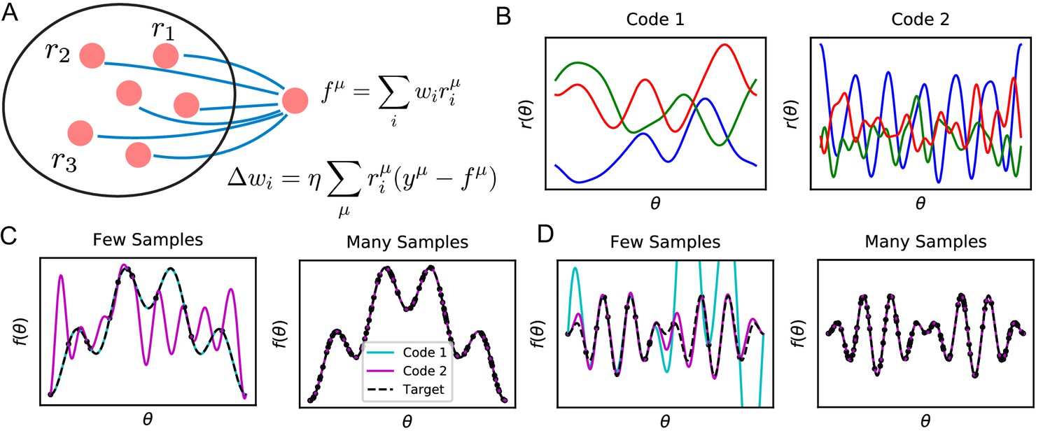
Learning tasks through linear readouts exploit representations of the population code to approximate a target response.
(A) The readout weights from the population to a downstream neuron, shown in blue, are updated to fit target values , using the local, biologically plausible delta rule. (B) Examples of tuning curves for two different population codes: Smooth tuning curves (Code 1) and rapidly varying tuning curves (Code 2). (C) (Left) A target function with low frequency content is approximated through the learning rule shown in A using these two codes. The readout from Code 1 (turquoise) fits the target function (black) almost perfectly with only training examples, while readout from Code 2 (purple) does not accurately approximate the target function. (Right) However, when the number of training examples is sufficiently large (), the target function is estimated perfectly by both codes, indicating that both codes are equally expressive. (D) The same experiment is performed on a task with higher frequency content. (Left) Code 1 fails to perform well with samples indicating mismatch between inductive bias and the task can prevent sample efficient learning while Code 2 accurately fits the target. (Right) Again, provided enough data , both models can accurately estimate the target function. Details of these simulations are given in Methods Generating example codes (Figure 1).
Figure 2
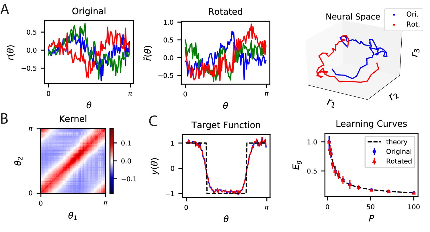
The inner product kernel controls the generalization performance of readouts.
(A) Tuning curves for three example recorded Mouse V1 neurons to varying static grating stimuli oriented at angle (Stringer et al., 2021; Pachitariu et al., 2019) (Left) are compared with a randomly rotated version (Middle) of the same population code. (Right) These two codes, original (Ori.) and rotated (Rot.) can be visualized as parametric trajectories in neural space. (B) The inner product kernel matrix has elements . The original V1 code and its rotated counterpart have identical kernels. (C) In a learning task involving uniformly sampled angles, readouts from the two codes perform identically, resulting in identical approximations of the target function (shown on the left as blue and red curves) and consequently identical generalization performance as a function of training set size (shown on right with blue and red points). The theory curve will be described in the main text.
Figure 3 with 1 supplement
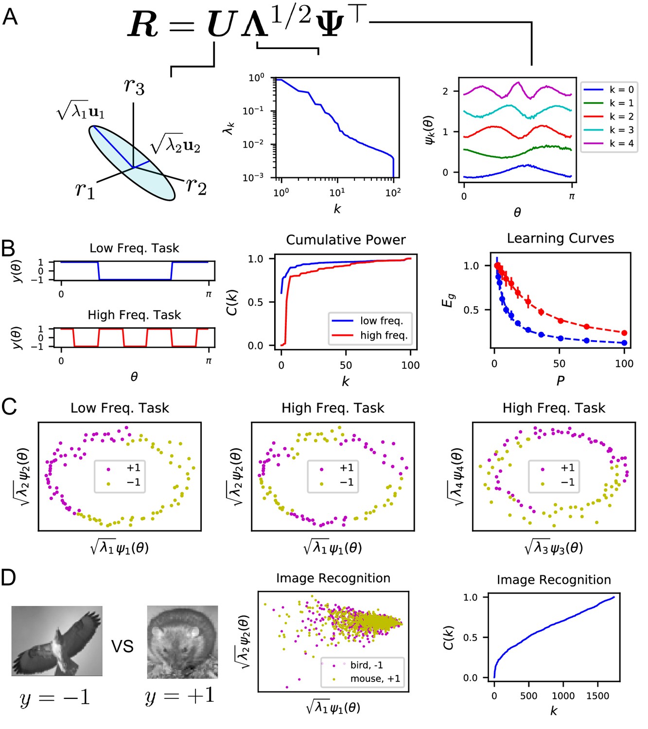
The singular value decomposition (SVD) of the population code reveals the structure and inductive bias of the code.
(A) SVD of the response matrix gives left singular vectors (principal axes), kernel eigenvalues , and kernel eigenfunctions . The ordering of eigenvalues provides an ordering of which modes can be learned by the code from few training examples. The eigenfunctions were offset by 0.5 for visibility. (B) (Left) Two different learning tasks , a low frequency (blue) and high frequency (red) function, are shown. (Middle) The cumulative power distribution rises more rapidly for the low frequency task than the high frequency, indicating better alignment with top kernel eigenfunctions and consequently more sample-efficient learning as shown in the learning curves (right). Dashed lines show theoretical generalization error while dots and solid vertical lines are experimental average and standard deviation over 30 repeats. (C) The feature space representations of the low (left) and high (middle and right) frequency tasks. Each point represents the embedding of a stimulus response vector along the -th principal axis . The binary target value is indicated with the color of the point. The easy (left), low frequency task is well separated along the top two dimensions, while the hard, high frequency task is not linearly separable in two (middle) or even with four feature dimensions (right). (D) On an image discrimination task (recognizing birds vs mice), V1 has an entangled representation which does not allow good performance of linear readouts. This is evidenced by the top principal components (middle) and the slowly rising curve (right).
Figure 3—figure supplement 1
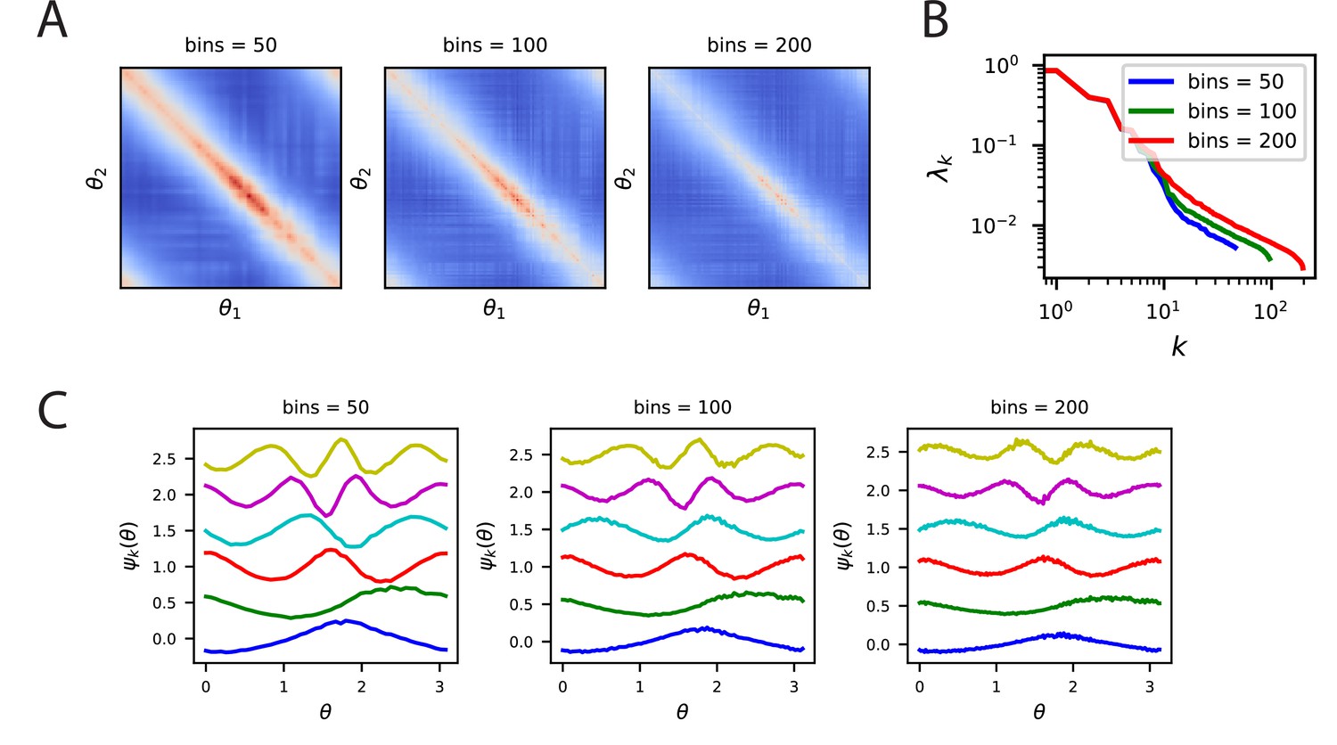
Kernels, spectra and eigenfunctions are well preserved across a variety of bin counts.
(A) The kernels for the V1 code where trial averaging is performed with 50, 100, 200 bins. (B) Despite the different bin values, the top eigenvalues are all very close, however, effects at the tail are visible. This is likely due to the reduction of trials per bin as the number of bins is increased. (C) Further, the top eigenfunctions are very similar for all bin counts. Since a higher number of bins means fewer trials to average over, the eigenfunctions for large bin count experiments are noisier.
Figure 4 with 1 supplement
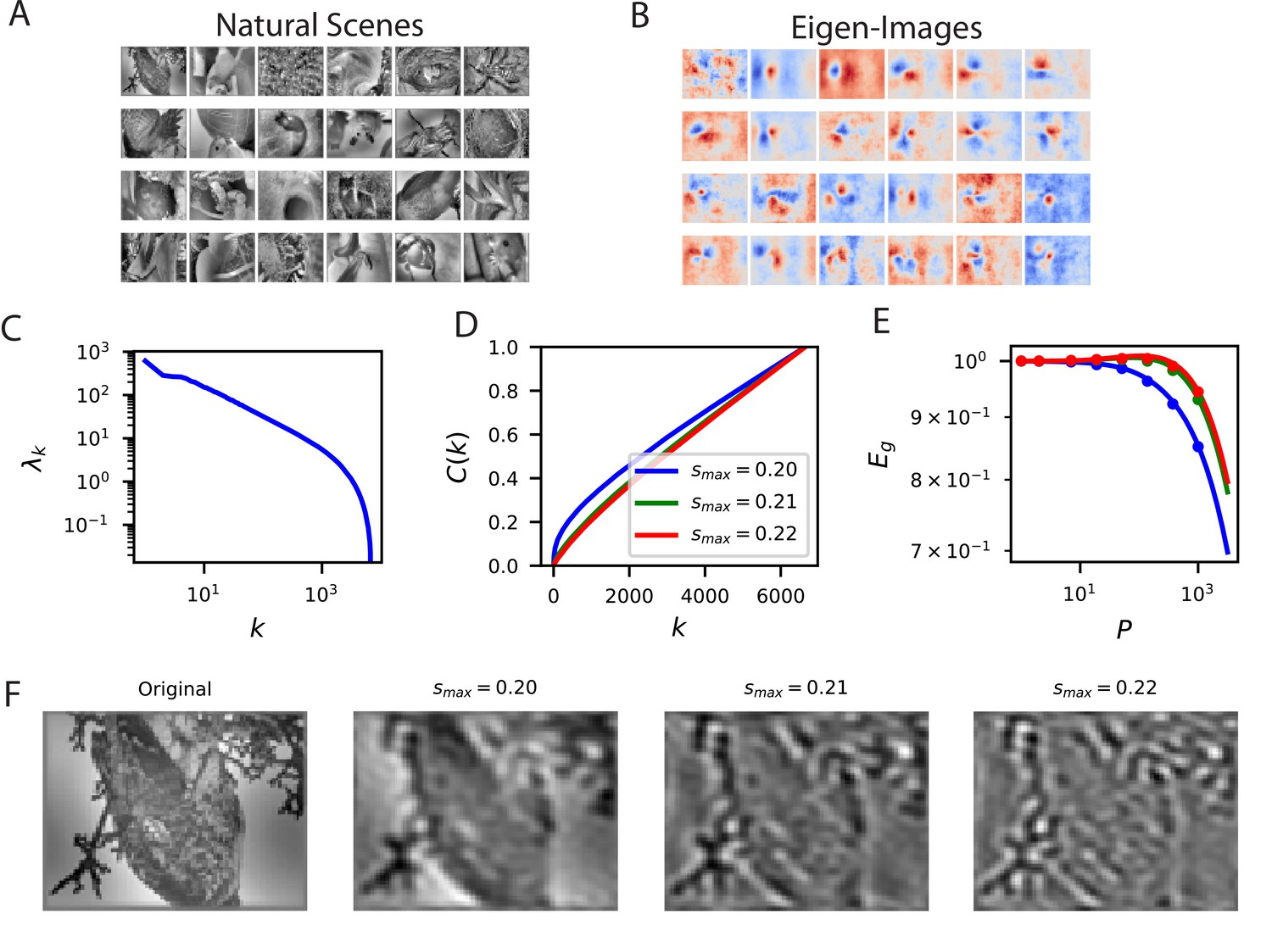
Reconstructing filtered natural images from V1 responses reveals preference for low spatial frequencies.
(A) Natural scene stimuli were presented to mice and V1 cells were recorded. (B) The images weighted by the top eigenfunctions . These “eigenimages" collectively define the difficulty of reconstructing images through readout. (C) The kernel spectrum of the V1 code for natural images. (D) The cumulative power curves for reconstruction of band-pass filtered images. Filters preserve spatial frequencies in the range , chosen to preserve volume in Fourier space as is varied. (E) The learning curves obey the ordering of the cumulative power curves. The images filtered with the lowest band-pass cutoff are easiest to reconstruct from the neural responses. (F) Examples of a band-pass filtered image with different preserved frequency bands.
Figure 4—figure supplement 1
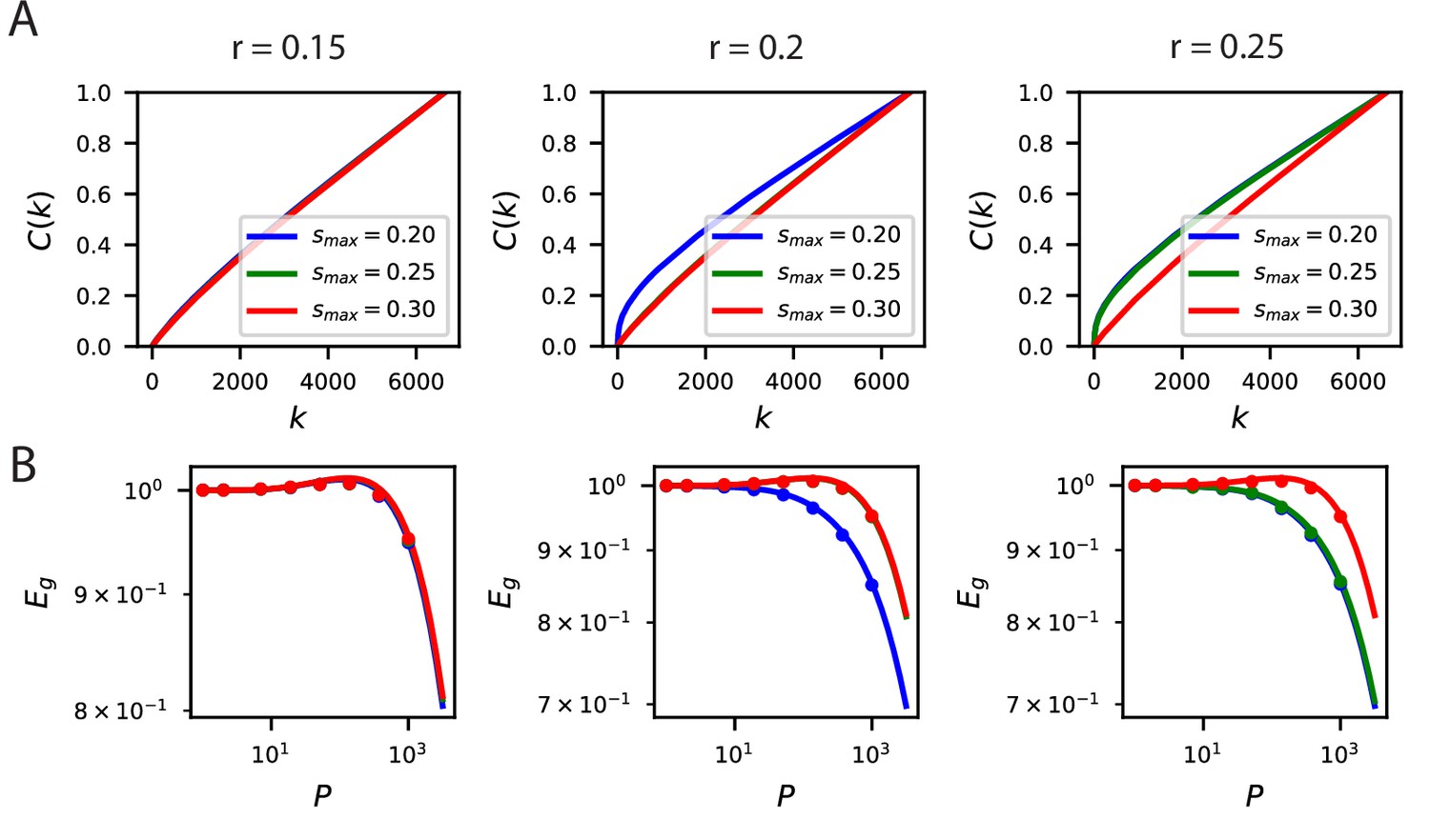
The inductive bias to reconstruct low spatial frequency components of natural scenes from the population responses holds over several band-pass filters of the form .
(A) The cumulative power curves for reconstruction of the filtered images with different values of and . Lower values of and higher values of preserve mostly low frequency content in the images and are easier to reconstruct from the neural responses. (B) The learning curves respect the ordering of the cumulative power metric .
Figure 5 with 3 supplements
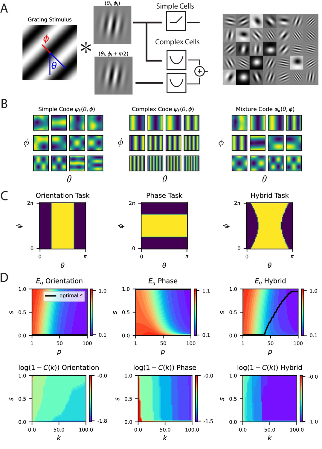
A model of V1 as a bank of Gabor filters recapitulates experimental inductive bias.
(A) Gabor filtered inputs are mapped through nonlinearity. A grating stimulus (left) with orientation and phase is mapped through a circuit of simple and complex cells (middle). Some examples of randomly sampled Gabor filters (right) generate preferred orientation tuning of neurons in the population. (B) We plot the top 12 eigenfunctions (modes) for pure simple cell population, pure complex cell population and a mixture population with half simple and half complex cells. The pure complex cell population has all eigenfunctions independent of phase . A pure simple cell population or mixture codes depend on both orientation phase in a nontrivial way. (C) Three tasks are visualized, where color indicates the binary target value ± 1. The left task only depends on orientation stimulus variable , the middle only depends on phase , the hybrid task (right) depends on both. (D) (top) Generalization error and cumulative power distributions for the three tasks as a function of the simple-complex cell mixture parameter .
Figure 5—figure supplement 1
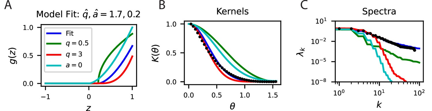
The fit of our simple cell model to the mouse V1 code.
(A) The fit nonlinearity has exponent and sparsifying threshold . These parameters are consistent with similar measurements in the cat visual cortex. We compare this nonlinearity to alternative codes with higher and lower and a code with the same but no threshold . (B) The fit parameters (blue) accurately fit the experimental kernel (black dots). (C) The spectra are also well predicted by the fit model.
Figure 5—figure supplement 2
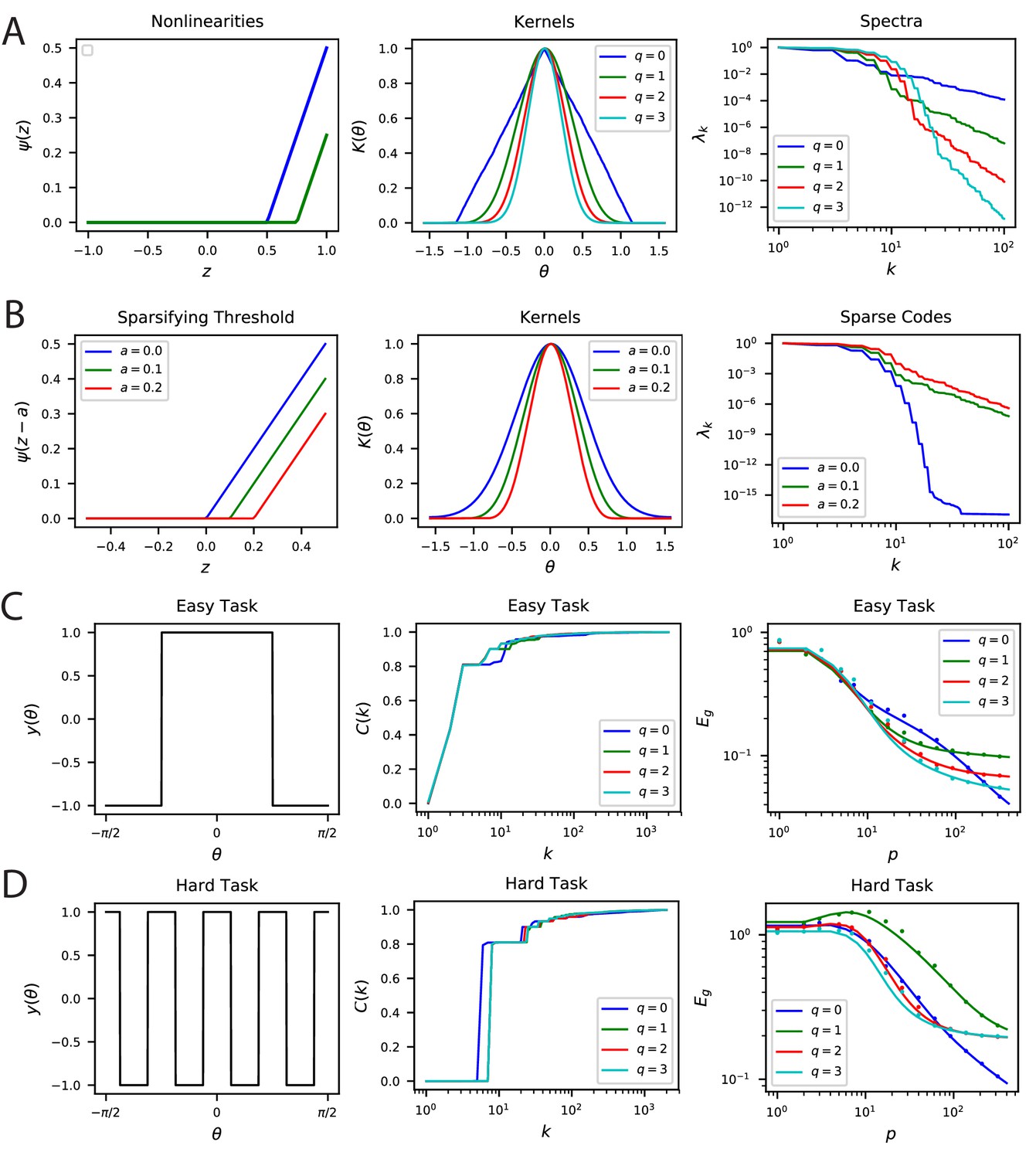
Nonlinear Rectification and proportion of simple and complex cells influences the inductive bias of the population code.
(A) The choice of nonlinearity has influence on the kernel and its spectrum. If the nonlinearity is , then . (B) The sparsity can be increased by shifting the nonlinearity . Sparser codes have higher dimensionality. Note that is a special case where the neurons behave in the linear regime for all inputs since the currents are positive. Thus, for , the spectrum decays like a Bessel Function for a constant . (C-D) Easy and hard orientation discrimination tasks with varying nonlinear polynomial order . At low sample sizes, large performs better, whereas at large , the step function nonlinearity achieves the best performance.
Figure 5—figure supplement 3
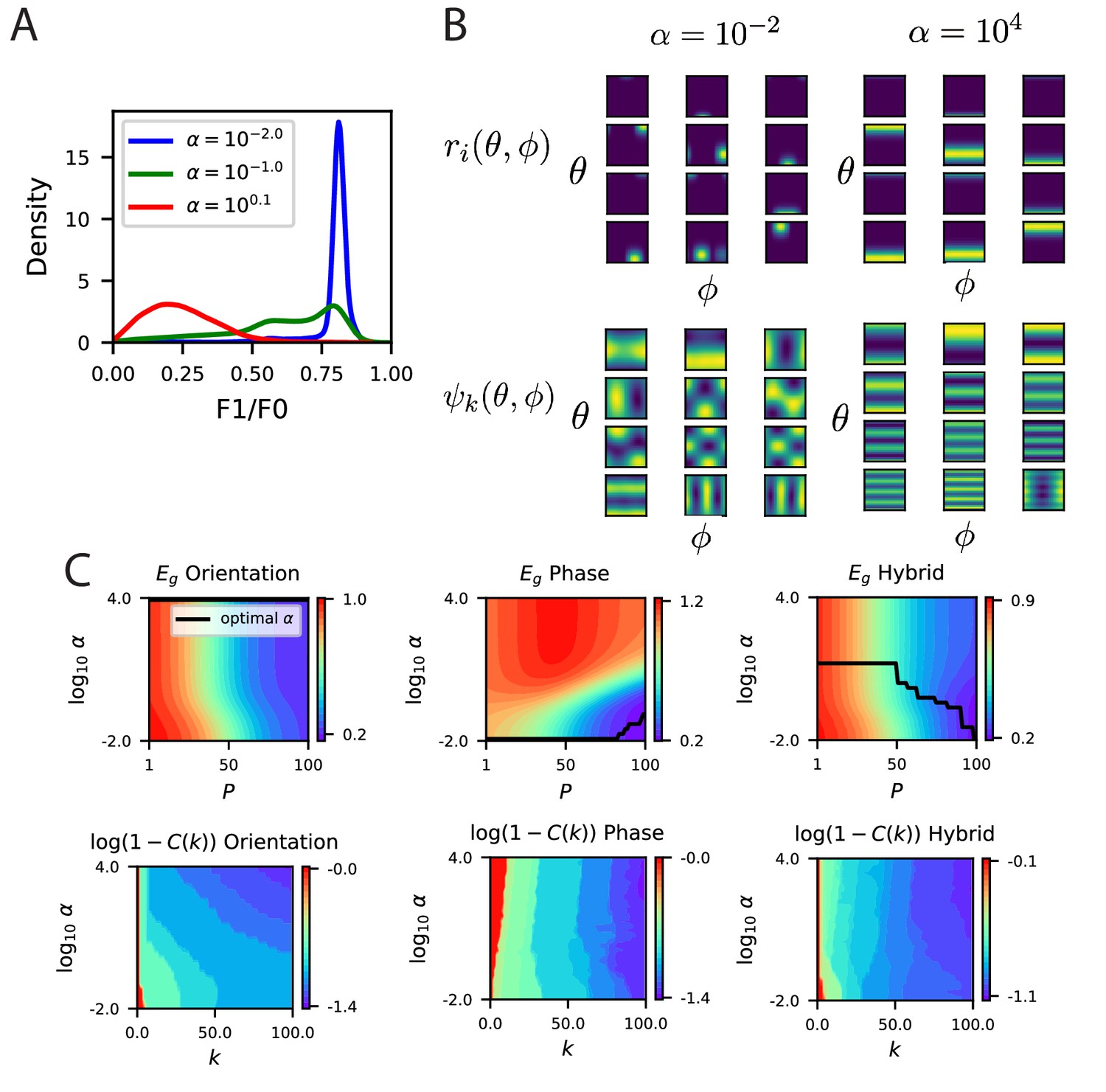
The modified energy based model with partial selectivity to phase reproduces the inductive bias of partial invariance.
(A) Some example F1/F0 distributions for various values of (Appendix Energy model with partially phase-selective cells). As the code becomes comprised entirely of complex cells. (B) Randomly selected tuning curves and the top 12 eigenfunctions for the modified energy model with and . As expected the code with smaller gives tuning curves with a variety of selectivity to phase variable , with some cells appearing more complex like and some appearing more like simple cells. At larger , all cells are approximately phase invariant. This heterogeneity in phase tuning at small and homogeneity at large are also reflected in the top eigenfunctions, which are phase dependent in the code but phase-invariant in the code. (C) The learning curves for the three tasks as a function of .
Figure 6 with 2 supplements

The top eigensystem of a code determines its low- generalization error.
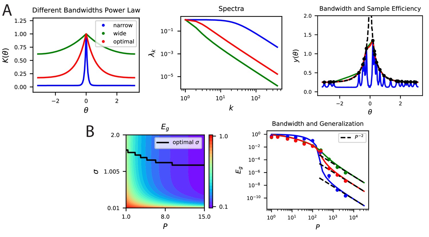
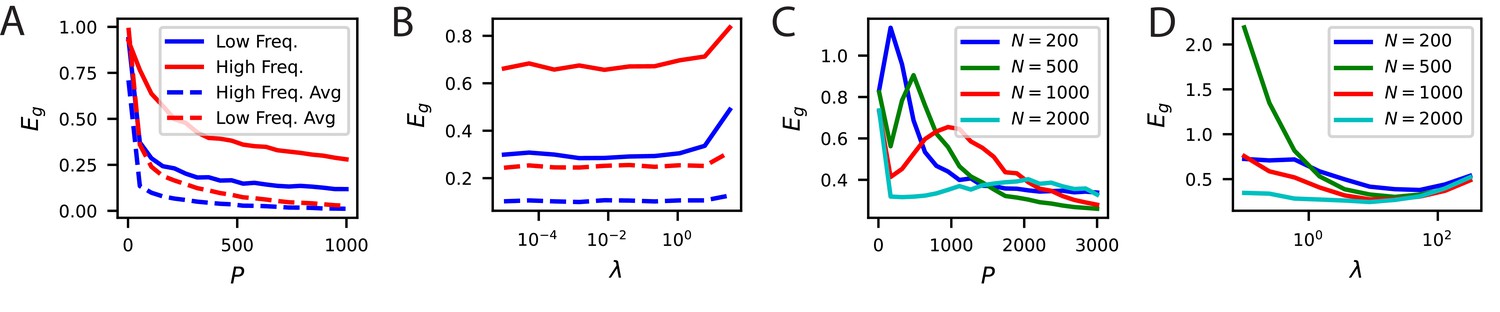
(A) A periodic variable is coded by a population of neurons with tuning curves of different widths (top). Narrow, wide and optimal refers to the example in C. These codes are all smooth (infinitely differentiable) but have very different feature space representations of the stimulus variable , as random projections reveal (below). (B) (left) The population codes in the above figure induce von Mises kernels with different bandwidths . (right) Eigenvalues of the three kernels. (C) (left) As an example learning task, we consider estimating a ‘bump’ target function. The optimal kernel (red, chosen as optimal bandwidth for ) achieves a better generalization error than either the wide (green) or narrow (blue) kernels. (middle) A contour plot shows generalization error for varying bandwidth and sample size . (right) The large generalization error scales in a power law. Solid lines are theory, dots are simulations averaged over 15 repeats, dashed lines are asymptotic power law scalings described in main text. Same color code as B and C-left.
Figure 6—figure supplement 1
Bandwidth (spectral bulk) also governs generalization in non-smooth codes.
(A, B) Kernel regression experiments are performed with Laplace kernels of varying bandwidth on a non-differentiable target function. The top eigenvalues are modified by changing the bandwidth, but the asymptotic power law scaling is preserved. Generalization at low is shown in the contour plot while the large scaling is provided in the generalization. In A-right and B-right, color code is the same as in the main text.
Figure 6—figure supplement 2
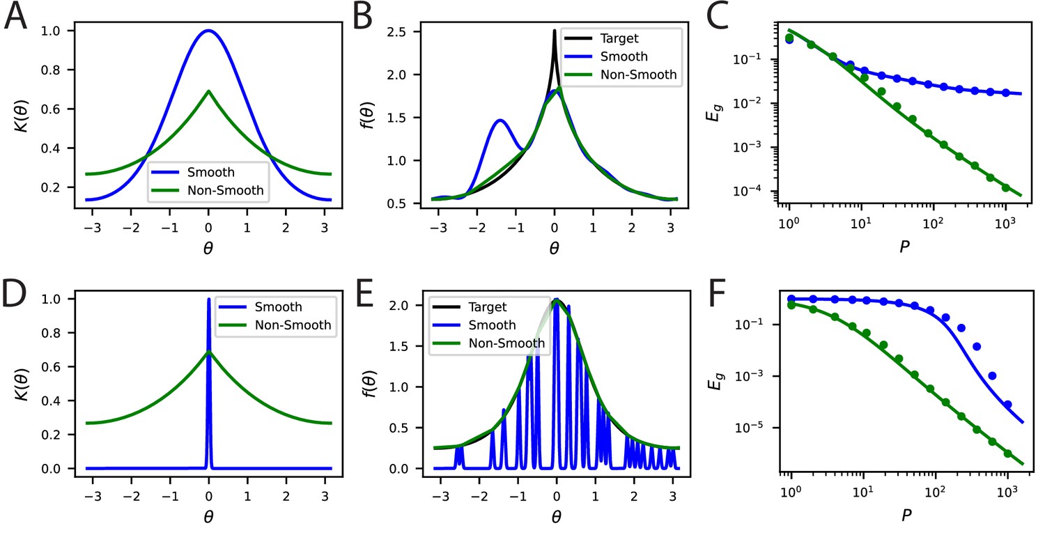
Non-differentiable kernels can generalize better than infinitely differentiable kernels in a variety of contexts.
(A) An infinitely differentiable von-Mises kernel (blue) will be compared to a non-differentiable Laplace kernel (green). (B) For a non-differentiable target function with a cusp, the non-smooth kernel can provide a better fit to the target function at samples. (C) The learning curves for this task. Solid lines are theory, circles are simulations. (D) The lengthscale of the kernel can be more important than local smoothness. We will now compare a narrow von-Mises kernel (still infinitely differentiable) with a non-differentiable wide kernel. (E) The non-smooth kernel generalizes on a smooth task almost perfectly whereas the narrow smooth kernel only locally interpolates. (F) The learning curves for this smooth task.
Figure 7
The performance of time-dependent codes when learning dynamical systems can be understood through spectral bias.
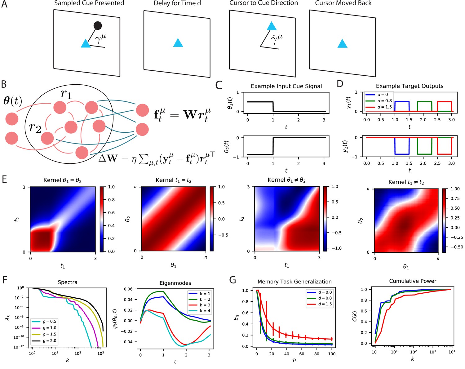
(A) We study the performance of time dependent codes on a delayed response task which requires memory retrieval. A cue (black dot) is presented at an angle . After a delay time , the cursor position (blue triangle) must be moved to the remembered cue position and then subsequently moved back to the origin after a short time. (B) The readout weights (blue) of a time dependent code can be learned through a modified delta rule. (C) Input is presented to the network as a time series which terminates at . The sequences are generated by drawing an angle and using two step functions as input time-series that code for the cosine and the sine of the angle (Methods RNN experiment, Appendix Time dependent neural codes). We show an example of the one of the variables in a input sequence. (D) The target functions for the memory retrieval task are step functions delayed by a time . (E) The kernel compares the code for two sequences at two distinct time points. We show the time dependent kernel for identical sequences (left) and the stimulus dependent kernel for equal time points (middle left) as well as for non-equal stimuli (middle right) and non-equal time (right). (F) The kernel can be diagonalized, and the eigenvalues determine the spectral bias of the reservoir computer (left). We see that higher gain networks have higher dimensional representations. The ‘eigensystems’ are functions of time and cue angle. We plot only components of top systems (right). (G) The readout is trained to approximate a target function , which requires memory of the presented cue angle. (left) The theoretical (solid) and experimental (vertical errorbar, 100 trials) generalization error are plotted for the three delays against training sample size . (right) The ordering of matches the ordering of the curves as expected.
Figure 8 with 2 supplements

The biological code is more metabolically efficient than random codes with same inductive biases.
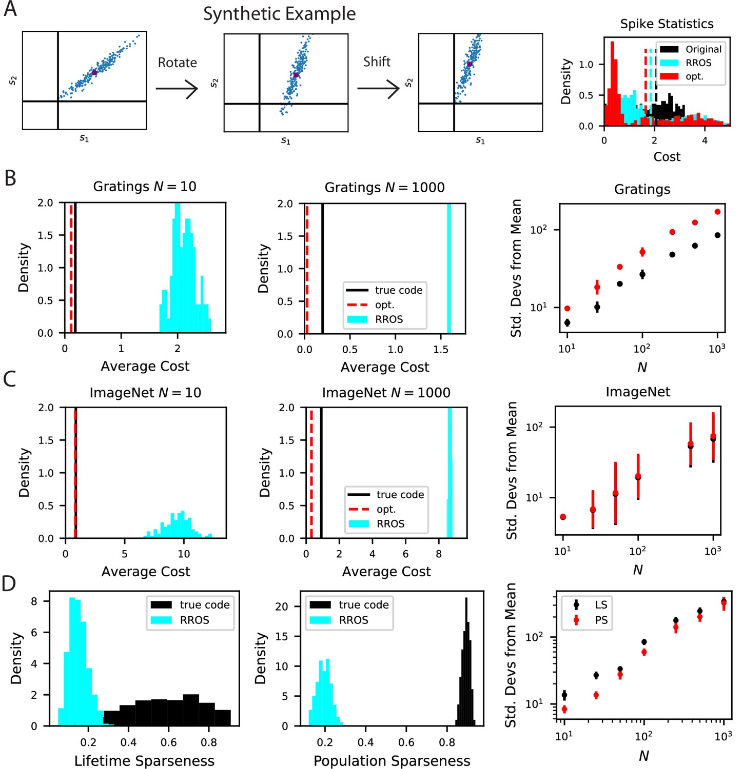
(A) We illustrate our procedure in a synthetic example. A non-negative population code (left) can be randomly rotated about its spontaneous firing rate (middle), illustrated as a purple dot, and optimally shifted to a new non-negative population code (right). If the kernel is measured about the spontaneous firing rate, these transformations leave the inductive bias of the code invariant but can change the total spiking activity of the neural responses. We refer to such an operation as random rotation + optimal shift (RROS). We also perform gradient descent over rotations and shifts, generating an optimized code (opt). (B) Performing RROS on neuron subsamples of experimental Mouse V1 recordings (Stringer et al., 2021; Pachitariu et al., 2019), shows that the true code has much lower average cost compared to random rotations of the code. The set of possible RROS transformations (Methods Generating RROS codes, and Methods Comparing sparsity of population codes) generates a distribution over average cost, which has higher mean than the true code. We also optimize metabolic cost over the space of RROS transformations, which resulted in the red dashed lines. We plot the distance (in units of standard deviations) between the cost of the true and optimal codes and the cost of randomly rotated codes for different neuron subsample sizes . (C) The same experiment performed on Mouse V1 responses to ImageNet images from 10 relevant classes (Stringer et al., 2018a; Stringer et al., 2018b). (D) The lifetime (LS) and population sparseness (PS) levels (Methods Lifetime and population sparseness) are higher for the Mouse V1 code than for a RROS code. The distance between average LS and PS of true code and RROS codes increases with .
Figure 8—figure supplement 1
Our metabolic efficiency finding is robust to different pre-processing techniques and upper bounds on neural firing.
(A) We show the same result as Figure 8 except we use raw (non -scored) estimate of responses for each stimulus. (B) Our result is robust to imposition of firing rate upper bounds ub on each neuron. This result uses the -scored responses to be consistent with the rest of the paper. The biological code achieves a maximum -score values in the range , which motivated the range of our tested upper bound values . (C) Our finding is robust to the number of sampled stimuli as we show in an experiment where rotations in dimensional subspace.
Figure 8—figure supplement 2
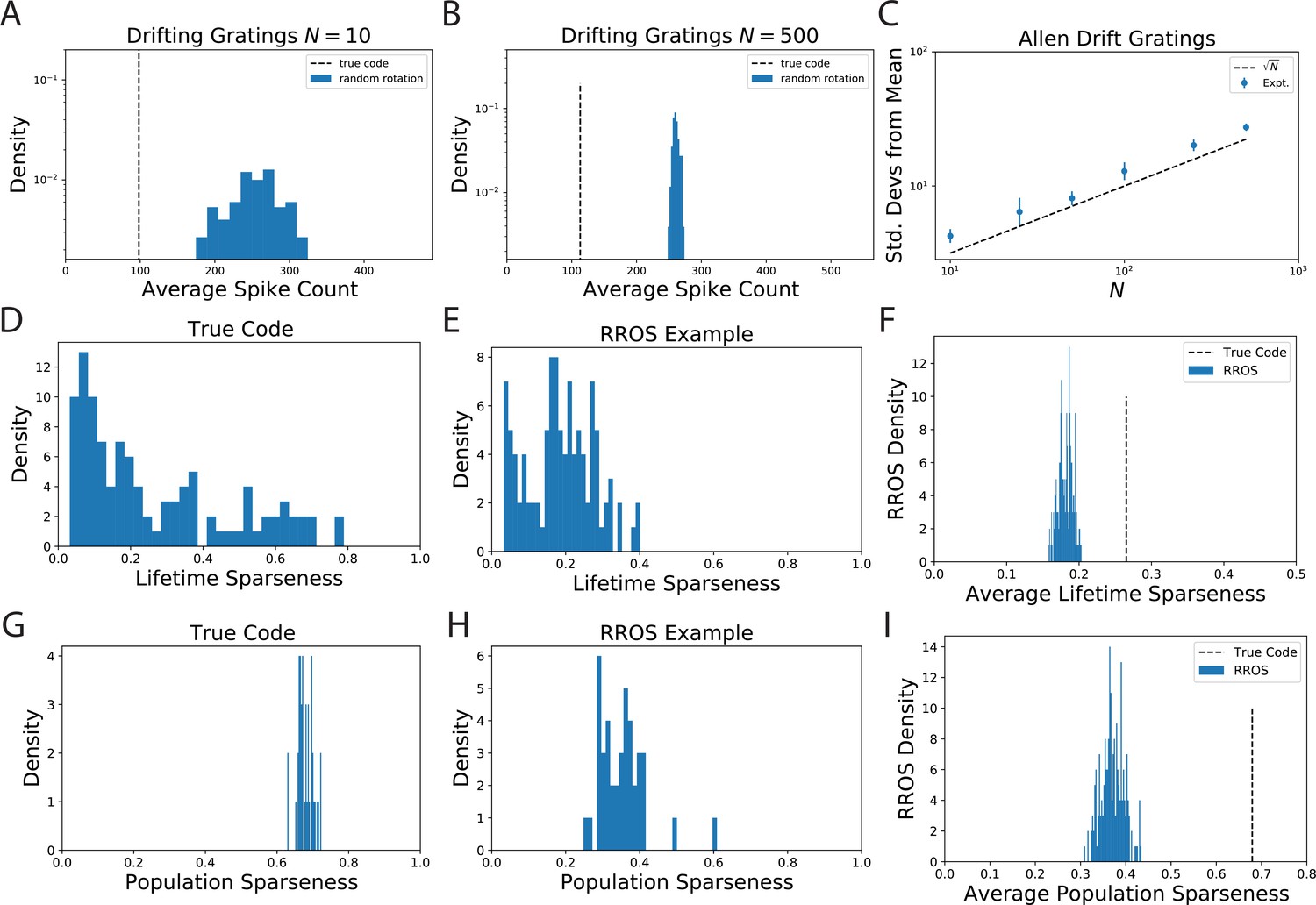
The observation that randomly oriented codes with the same kernel require higher spike counts than the original code is reproduced from electrophysiological recordings of Mouse visual cortex (VISp and VISal) from the AIBO.
(A) Distribution of average spike count for a random selection of neurons. (B) The same for randomly selected neurons. (C) Since the distribution of average spike count for the randomly rotated codes concentrates with the number of standard deviations the true code is from the mean increases with . We show that this scaling is approximately like which suggests that the variability in average spike count for randomly rotated codes goes scales with neuron count like . This is intuitive since the average spike count over the rotated code is an empirical average over random variables. (D) The lifetime sparseness of neurons in the true code are spread out over a large range. (E) The lifetime sparseness distribution for an example RROS code does not have the same range. (F) The average (over neurons) lifetime sparseness of RROS codes over random rotations is significantly lower than the average lifetime sparseness of the true code. (G-I) The true visual cortex code has much higher population sparseness over each grating stimulus as well.
Appendix 1—figure 1
Neural noise and subsampled neural codes can lead to overfitting.
(A) The learning curves without trial averaging (solid) and with trial averaging (dashed) for the high and low frequency orientation discrimination task. In principle, neural noise could limit asymptotic performance and lead to the existence of an optimal weight decay parameter . (B) Performance at vs ridge shows that there is not an optimal weight decay parameter. (C) Generalization of readouts trained on subsets of V1 neurons exhibit non-monotonic learning curves with an overfitting peak around . (D) The performance of subsamples of neurons as a function of the weight decay parameter at samples show that, for sufficiently small , there is a non-zero optimal .
Additional files
Download links
A two-part list of links to download the article, or parts of the article, in various formats.
Downloads (link to download the article as PDF)
Open citations (links to open the citations from this article in various online reference manager services)
Cite this article (links to download the citations from this article in formats compatible with various reference manager tools)
Population codes enable learning from few examples by shaping inductive bias
eLife 11:e78606.
https://doi.org/10.7554/eLife.78606


