Eco-evolutionary dynamics of clonal multicellular life cycles
- Max Planck Institute for Evolutionary Biology, Germany
- Hamburg Center for Health Economics, University of Hamburg, Germany
- Department of Ecology and Evolutionary Biology, Princeton University, United States
Figures
Figure 1
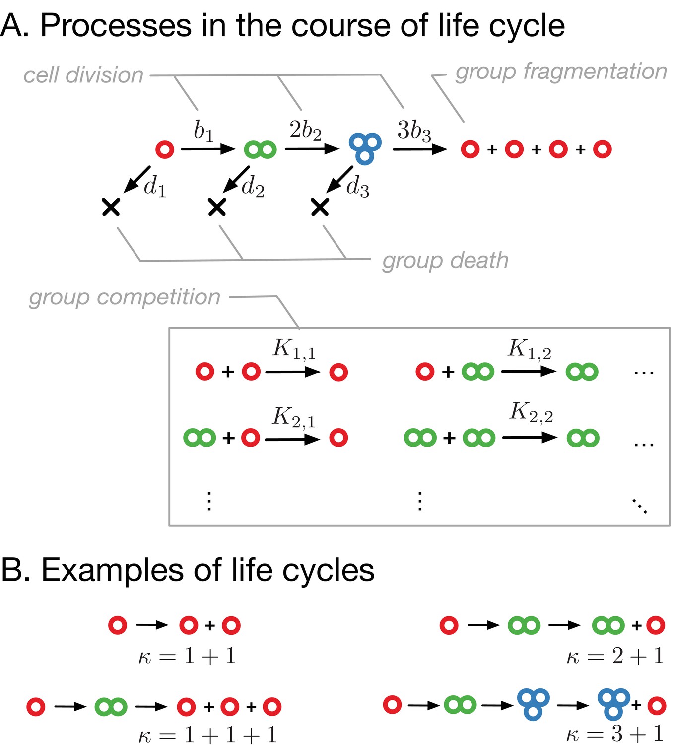
Model of clonal life cycles.
(A) There are four processes occurring in the model: groups grow by cell division, which occurs with rates , groups spontaneously die with rates , groups fragment immediately upon exceeding maturity size (3 in this example), according to predefined fragmentation pattern (1 + 1 + 1 + 1 here), and groups of size die due to the competition with groups of size at rates . (B) Together, group growth and fragmentation constitute a life cycle, in which initially small groups grow in size and eventually fragment, giving rise to more small groups. Colors represent group sizes: red, solitary cells; green, bicellular groups; blue, tricellular groups.
Figure 2

A single life cycle comes to a stationary state.
(A) For a unicellular life cycle , our model is equivalent to logistic growth. There, the number of solitary cells (red) approaches the carrying capacity from any initial state. (B, C) For multicellular life cycles (2 + 1 depicted), the population also approaches such a stationary state from any initial state. (B) shows the dynamics of solitary cells (red) and bicellular groups (green) with time. (C) shows the trajectories of the population composition, the dot marks the stationary state. (B) and (C) show the same dataset.
Figure 3
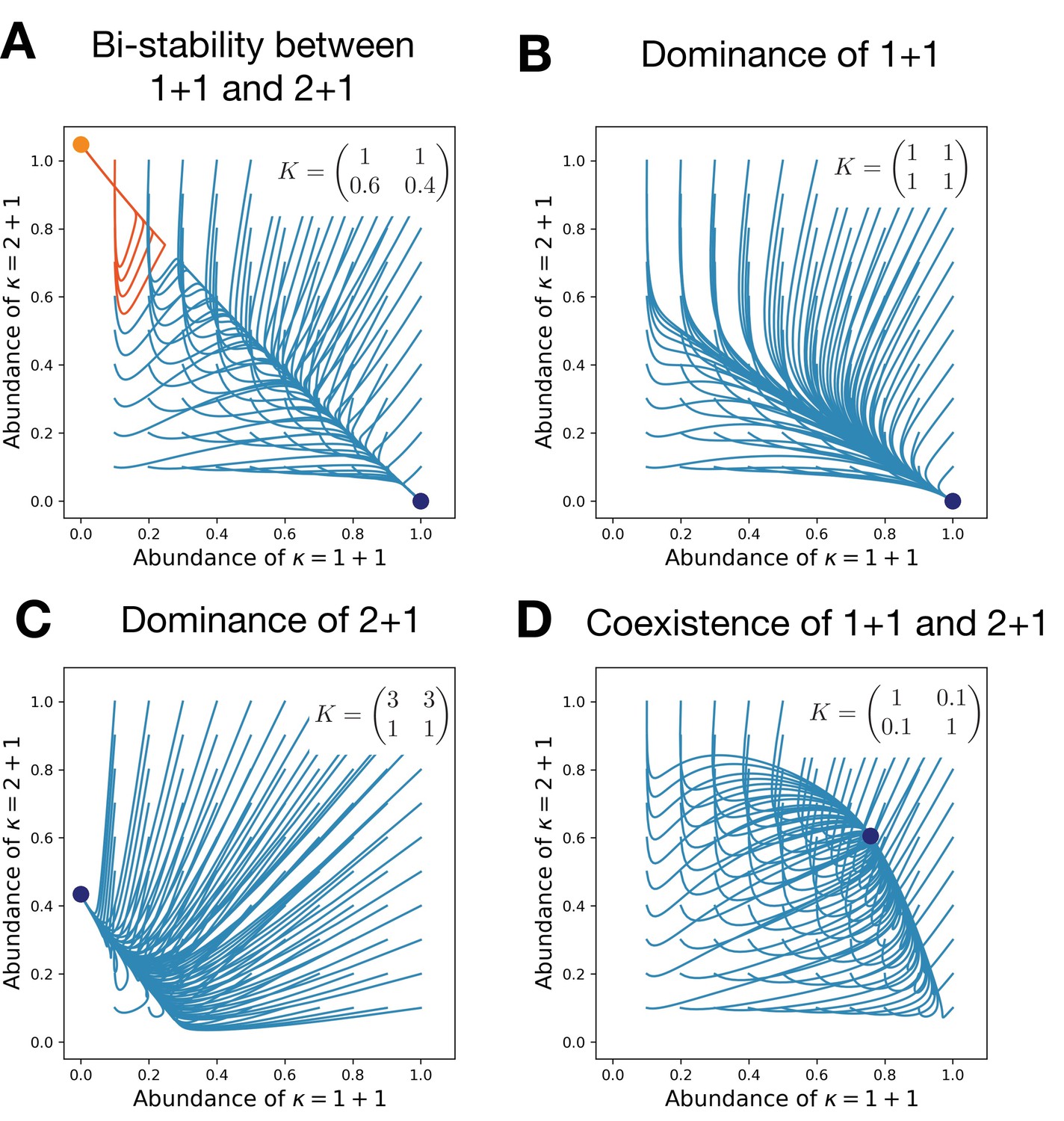
Competitive interactions can lead to the bistability between life cycles (A), a dominance of either of them (B,C), or their coexistence (D).
Each panel shows the evolutionary trajectories of populations with various initial abundances of the life cycles 1 + 1 and 2 + 1 (lines) and all final states (dots). In (A), colors indicate to which of two stationary states the trajectory converges. Birth and death rates are and ; they favor the unicellular life cycle 1 + 1 in the absence of competition. Simulations performed on each panel only differ in the competition matrix K shown in panels.
Figure 4
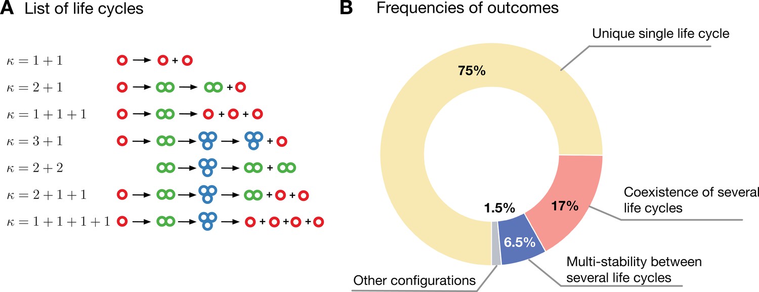
Evolution in a population with multiple competing life cycles.
(A) The schematics of the life cycles taking part in evolution. Groups colored according to the number of cells. (B) The frequencies of various classes of outcomes. A single life cycle (yellow) is the most common. Coexistence of life cycles (red) and bistability between them (blue) are less common. More complex composite configurations (gray) are also possible, but found rarely.
Figure 5
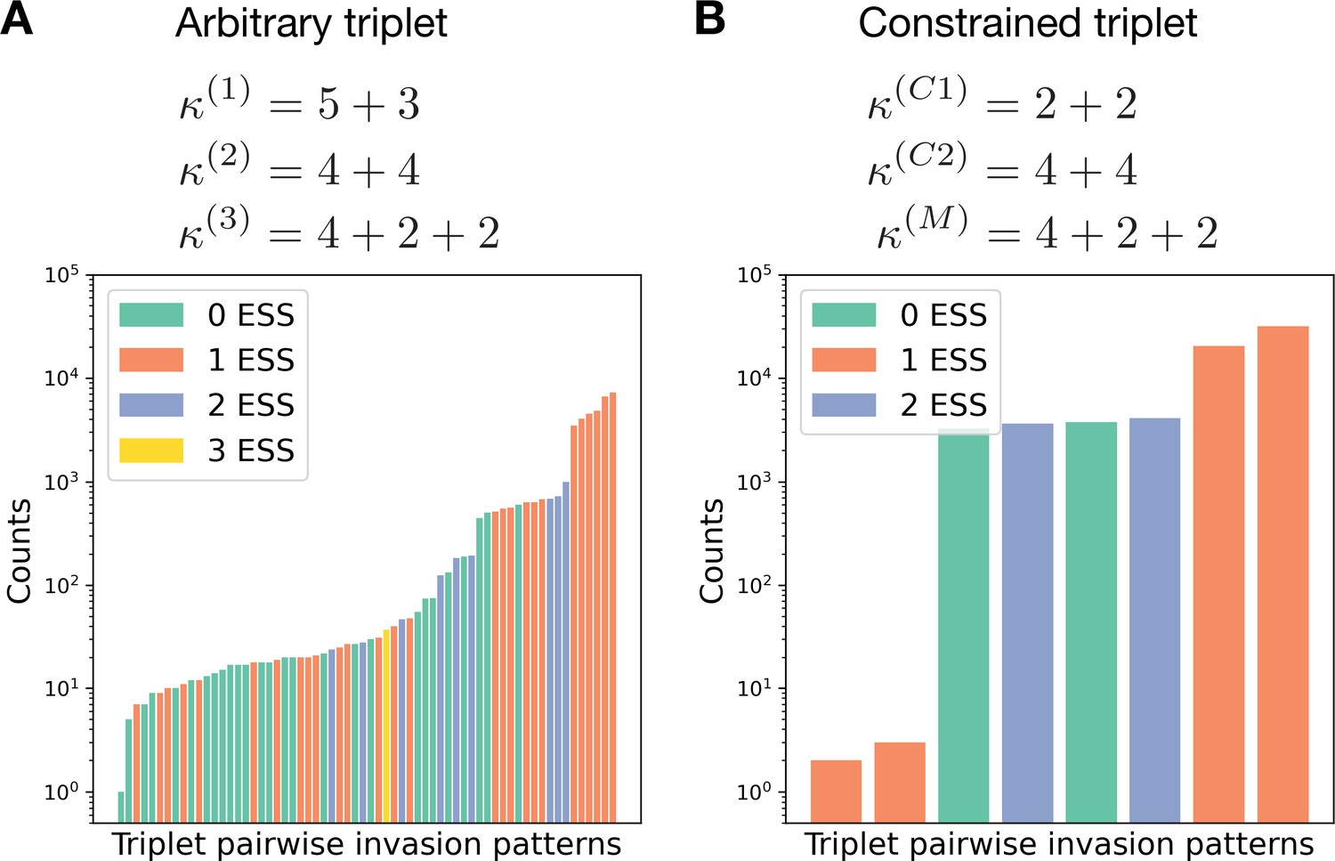
Constrained triplets demonstrate fewer patterns of pairwise invasion.
(A) For a combination of three life cycles, there are pairwise invasion patterns possible. For the triplet , the rates of all processes () were randomly sampled from an exponential distribution with unit rate parameter. Then the pairwise invasion pattern was identified. All 64 possible patterns were observed in these simulations. (B) In a similar investigation for the triplet , in which and constrain , only eight patterns were found; see the main text for a discussion.
Figure 6
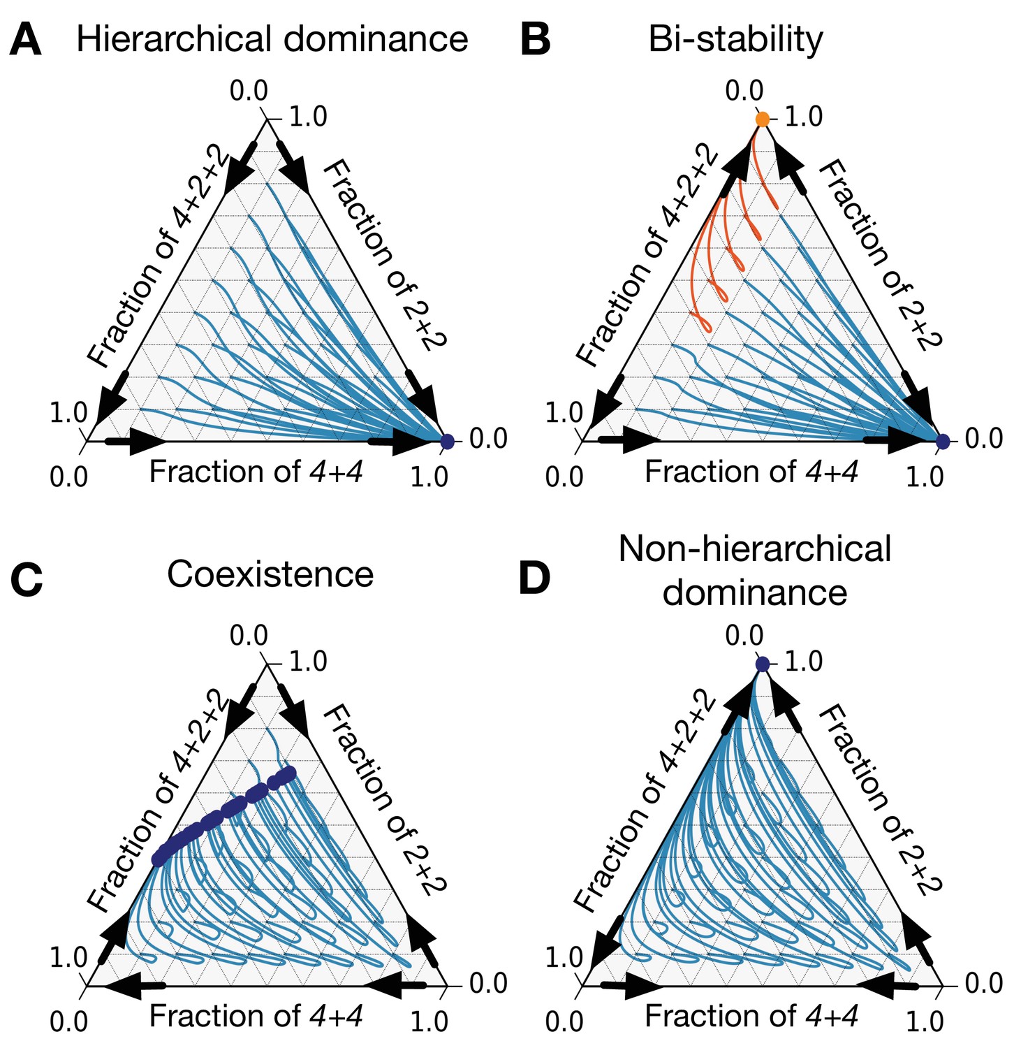
There are only eight patterns of pairwise invasion in a constrained triplet of life cycles.
Four patterns are shown here and four more are symmetric to them. Blue lines are population dynamics trajectories with different initial composition of the population. Red points are final states. Black arrows show directions of invasion from rare. (A) In a hierarchical dominance, one of the constraining life cycles outcompetes the two others from any initial condition. (B) In a bistability situation, each of the two constraining life cycles is able to outcompete the third life cycle. Which of them will survive depends on the initial conditions. Trajectories converging to different stationary states are highlighted with different colors. (C) In a coexistence, all three life cycles survive to a stationary state. (D) In a non-hierarchical dominance, one of the constraining life cycles outcompetes another; however, in the abundance of the constrained life cycle, the dominance is reversed. The parameters used to produce these figures are presented in Appendix 5.
Tables
Table 1
Competitive interactions in a pair of life cycles can lead to the dominance of either life cycle, their coexistence, or bistability.
cannot invade into | can invade into | |
|---|---|---|
| cannot invade into | Bistability between and | Dominance of |
| cannot invade into | Dominance of | Coexistence of and |
Table 2
Observation frequencies of different kinds of evolutionary outcomes in a population with multiple competing life cycles.
| Outcome | Frequency | |
|---|---|---|
| Single life cycle | 0.751 | |
| Coexistence of | Two life cycles | 0.121 |
| Three life cycles | 0.044 | |
| Four or more life cycles | 0.003 | |
| Multistability between | Two life cycles | 0.065 |
| Three life cycles | 0.002 | |
| Four or more life cycles | 0 | |
| Composite configurations | Bistability with a coexisting pair | 0.007 |
| Other configurations | 0.007 | |
Additional files
Download links
A two-part list of links to download the article, or parts of the article, in various formats.
Downloads (link to download the article as PDF)
Open citations (links to open the citations from this article in various online reference manager services)
Cite this article (links to download the citations from this article in formats compatible with various reference manager tools)
Eco-evolutionary dynamics of clonal multicellular life cycles
eLife 11:e78822.
https://doi.org/10.7554/eLife.78822


