The unmitigated profile of COVID-19 infectiousness
- Weizmann Institute of Science, Israel
- Department of Ecology and Evolutionary, Princeton University, United States
- Department of Biology, McMaster University, Canada
- Department of Mathematics and Statistics, McMaster University, Canada
- M. G. DeGroote Institute for Infectious Disease Research, McMaster University, Canada
Figures
Figure 1

Definitions of epidemiological time intervals.
The incubation period is defined as the time between infection and symptom onset (= for the infector, for the infectee). The serial interval (=) is defined as the interval between the onset of symptoms of two subsequent transmission events (infector and infectee) and the generation interval is the time lapse between the infections of those individuals (= ). TOST stands for time from onset of symptoms to transmission (Ferretti et al., 2020b), and is defined accordingly as the time lapse between symptom onset in the infector and the infection of the infectee (i.e., transmission time). The timeline at the bottom corresponds to the notation used in the Methods section.
Figure 2
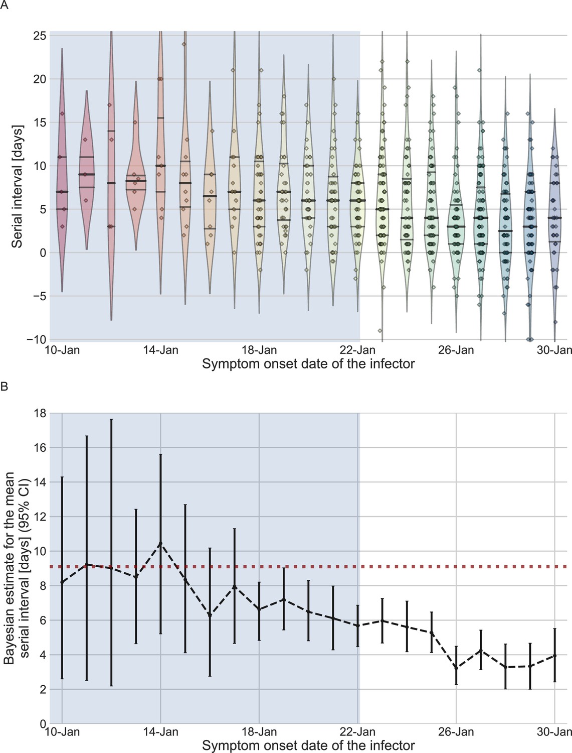
The serial-interval dataset and the estimates of its mean during the early-outbreak period.
(A) The empirical distributions of forward serial intervals in the combined dataset, grouped based on the symptom-onset dates of the infectors and visualized using a violinplot. For pairs with uncertainty regarding the exact dates of symptom onset, we used a date in the middle of the uncertainty range. The violin shapes represent a kernel density estimation of the underlying distribution. The median and interquartile range (percentiles 25–75) are presented using dotted horizontal lines within the shape. The diamonds represent the data points for each of the dates of infector symptom onset. The dataset contains transmission pairs with infectors who developed symptoms from December 12 onward. Dates prior to January 10 are not shown as the data are too sparse. (B) The estimates of the mean serial interval, based on a parametric Bayesian inference (see Supplementary Information for details). The error bars represent the 95% confidence interval (CI) of the estimates. The dashed horizontal line represents the observed mean serial interval for the period up to January 17. Dates up to January 17, 2020, are highlighted in both panels as they represent the period of unmitigated transmission.
Figure 3 with 1 supplement
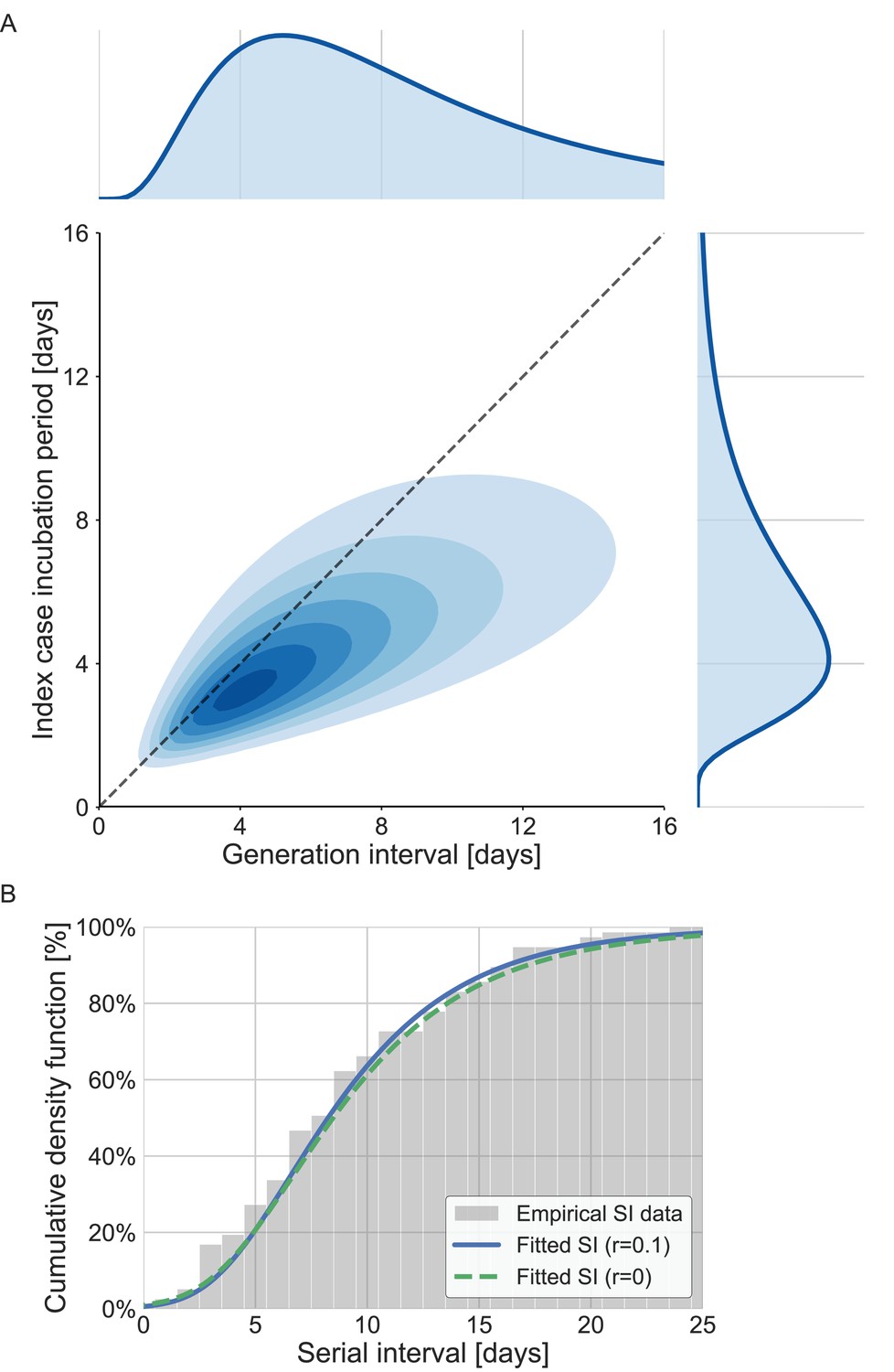
The joint distribution of generation interval and incubation period.
Representations of the inferred joint distribution results are based on maximum likelihood analysis. (A) The joint bivariate distribution (bottom left graph), shown as contours over the plane of generation intervals (x-axis) and incubation period distribution (y-axis). The correlation parameter (in log space, see Methods) was found to be 0.75 (0.5–0.9 95% confidence interval [CI]). The panel also shows the univariate components of the joint distribution: the generation-interval distribution (top graph, sharing the same x-axis) and the incubation period distribution (bottom right graph, sharing the same y-axis). The incubation period distribution was assumed to follow a lognormal distribution with a shape parameter of 0.53 and a scale parameter of 5.5 days, following Xin et al., 2021. The dashed diagonal line describes equal incubation period and generation interval (time from onset of symptoms to transmission [TOST] equal to zero). Left of this line could be found the pre-symptomatic fraction of transmission. (B) Cumulative histogram of the empirical serial intervals and the parametric distribution derived from the maximum likelihood joint distribution. The estimated serial-interval distribution was derived using the likelihood calculation given the reported growth rate of r=0.1 day–1 (Tsang et al., 2020). For comparison the dashed line represents the intrinsic serial interval distribution, estimated by Equation (2) with the parameters derived from the maximum likelihood analysis (corresponding to the case of r=0 day–1).
Figure 3—figure supplement 1
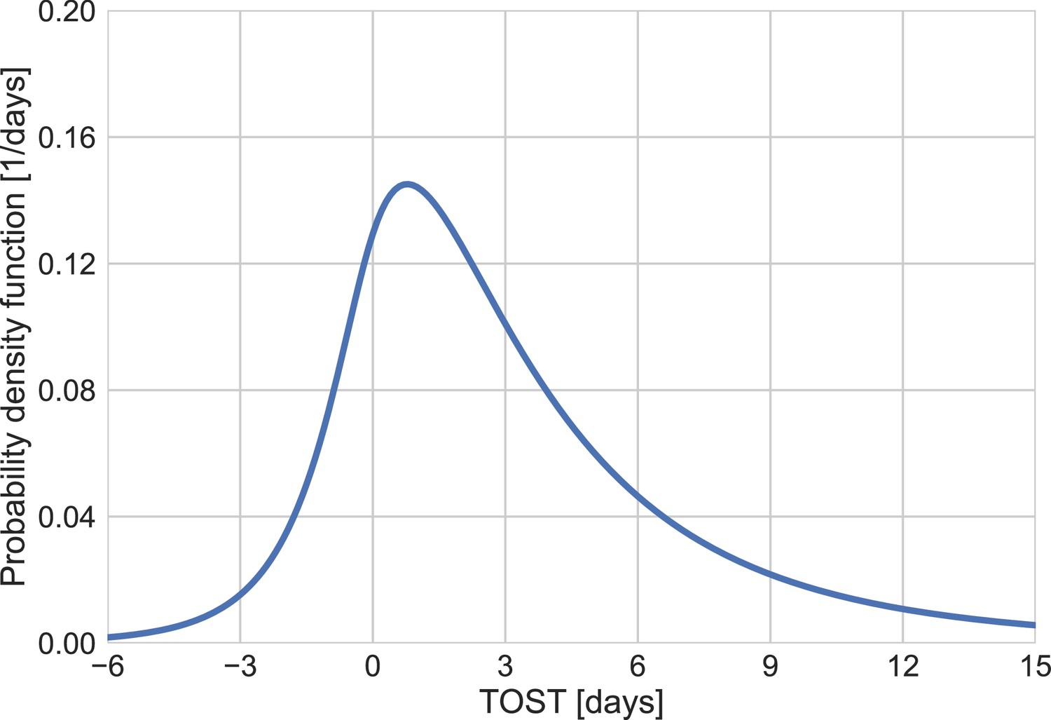
The distribution of time from onset of symptoms to transmission (TOST).
Derived from the joint bivariate lognormal distribution.
Figure 4 with 1 supplement

Comparison of the mean generation-interval distribution with those of previous studies.
The generation-interval distribution inferred by maximum likelihood presented alongside available estimates from the literature (Ferretti et al., 2020a; He et al., 2020; Johansson et al., 2021; Lauer et al., 2020; Sun et al., 2020). (A) The probability density functions of the distributions. The legend reports the median and standard deviation of each of the distributions. (B) The survival function of the generation-interval distribution, defined as the complement of the cumulative distribution, representing the residual fraction of transmission after a designated time since infection. The inset shows a zoom-in on the period of 12–24 days after exposure, a period in which there is a substantial difference between the current estimate and those from previous studies. The highlighted area represents the 95% confidence interval of the maximum likelihood estimate.
Figure 4—figure supplement 1
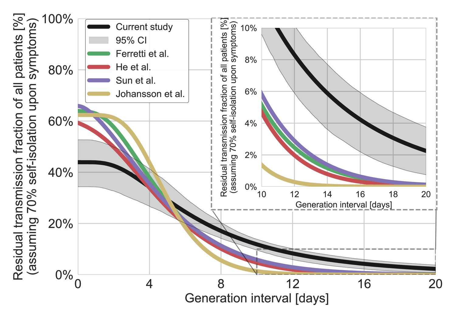
The residual transmission accounting for self-isolation.
The residual transmission under the conjecture that 70% of individuals self-isolate upon the development of symptoms was calculated as a weighted average of the regular survival function (shown in Figure 4B) and the residual transmission conditioned on the self-isolation function. This analysis was performed for the distribution of generation intervals inferred by maximum likelihood as well as for best available estimates from the literature (Ferretti et al., 2020a; He et al., 2020; Johansson et al., 2021; Lauer et al., 2020; Sun et al., 2020). The residual transmission conditioned on self-isolation function is calculated through the integration of the bivariate distribution of incubation period and generation interval, on the relevant quadrant (the probability summed on incubation and generation interval greater than a specific value). The inset shows a zoom-in on the period of 10–20 days after exposure, a period in which there is a substantial difference between the current estimate and those from previous studies. The highlighted area represents the 95% confidence of the maximum likelihood estimate.
Figure 5 with 3 supplements
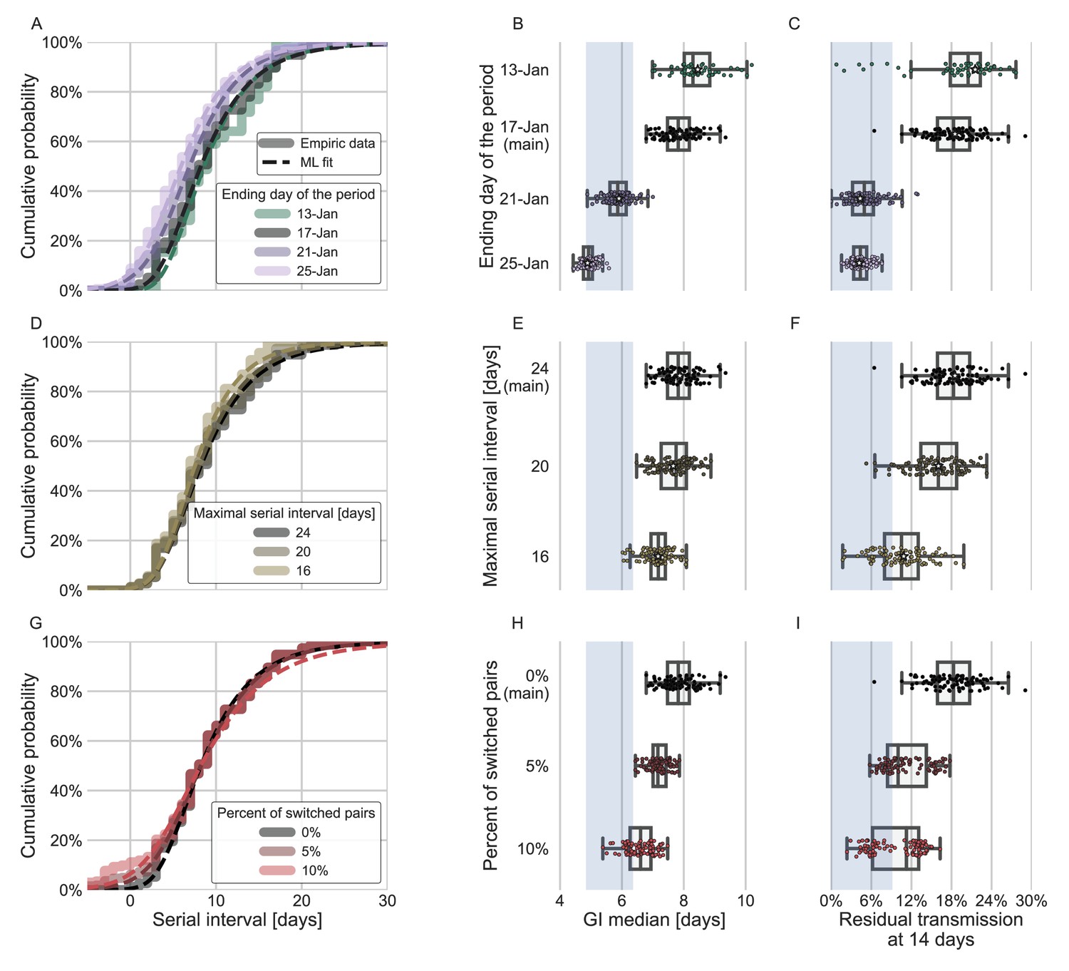
Sensitivity analyses of the inferred generation interval.
A comparison of the results of sensitivity analysis to three factors: the period chosen to represent the unmitigated transmission (A–C), the inclusion of the longest serial intervals in the dataset (D–F), and the ordering of the transmission pairs (G–I). (A, D, G) Cumulative histogram of the empirical serial intervals and the parametric distribution derived from the maximum likelihood joint distribution. The estimated serial interval distribution was derived using the likelihood calculation given the reported growth rate of r=0.1 day–1 (Tsang et al., 2020). (E, H) Best estimates and distributions of the resulting median of the inferred generation-interval distribution. A black star marks best estimates. Ranges are given as boxplots. The box represents the interquartile range (percentiles 25–75) and the whiskers represent the maximal range of the distribution apart from outliers (defined as data points exceeding the interquartile range by a factor of 1.5). Each dot represents a single bootstrapping iteration. The blue shaded region represents the values from previous studies (Ferretti et al., 2020a; He et al., 2020; Sun et al., 2020; Tsang et al., 2020). (F, I) Best estimates and distributions of the resulting residual transmission at 14 days since infection derived from the inferred generation-interval distribution. The best estimates and ranges are shown in the same manner as the distribution parameters in panels E, H.
Figure 5—figure supplement 1
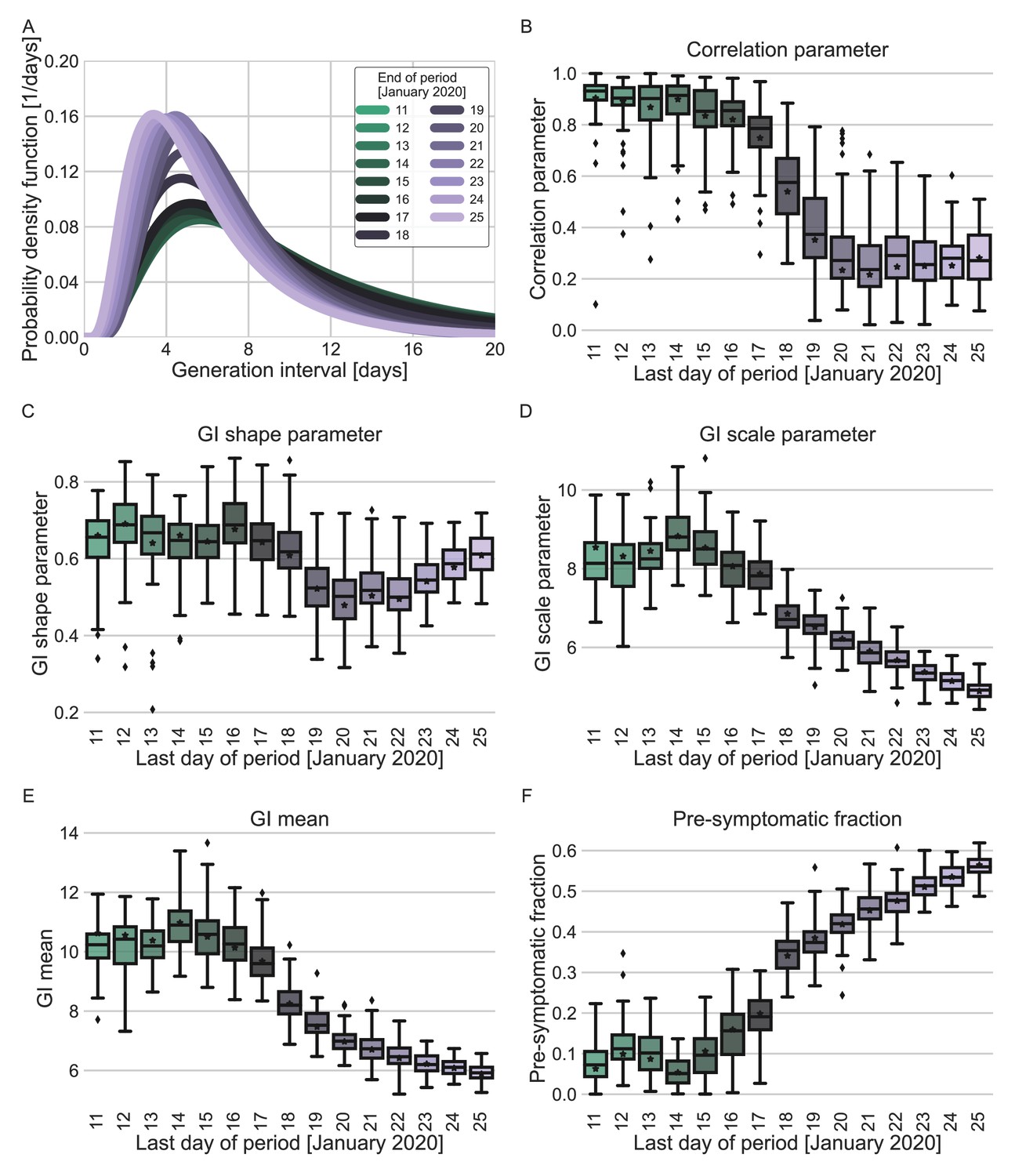
Sensitivity analysis regarding the choice of period for analysis.
Maximum likelihood estimates of the bivariate incubation period and generation-interval distribution were made for datasets containing the transmission pairs with infector onset date up to a specific date. Best estimates were derived for each of the datasets. Uncertainty estimates were derived by bootstrapping, through sampling with replacement from the dataset and sampling from the distribution of growth rates (Tsang et al., 2020). (A) Best estimate for the generation-interval distribution probability density function for periods ending at dates in the range of 11–25 (Zhao et al., 2020). (B–D) Best estimates and distributions of the resulting parameters of the bivariate distribution of incubation period and generation interval. A black star marks best estimates. Ranges are given as boxplots. The box represents the interquartile range (percentiles 25–75) and the whiskers represent the maximal range of the distribution apart from outliers (defined as data points exceeding the interquartile range by a factor of 1.5). (E–F) The mean generation interval and the fraction of pre-symptomatic transmission, derived from the results. The best estimates and ranges are shown in the same manners as the distribution parameters in panels B–D.
Figure 5—figure supplement 2
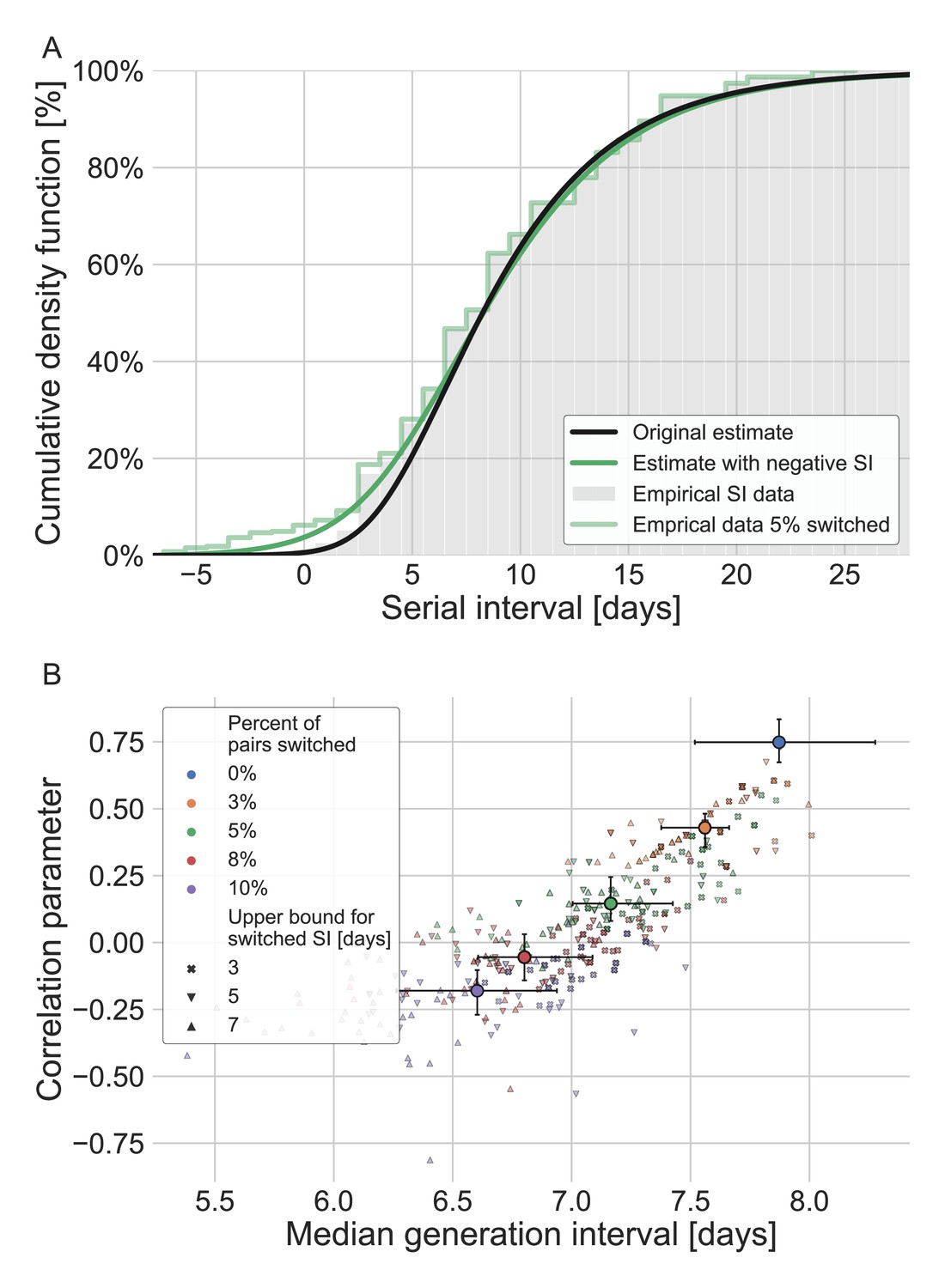
Estimates for the bivariate incubation period and generation-interval distribution were obtained for adjusted datasets in which the order of transmission was switched between the infector and infectee (giving a negative serial interval).
Error bar represent the interquantile range (quntiles 25%-75%) of the results. The analysis was performed by varying the fraction of pairs switched (0–0.1) and the maximal serial interval for which order switching is allowed (3–7 days). For each combination, the analysis was run 30 times while switching the pairs at random. (A) The serial interval cumulative distribution averaged over all (90) runs with 5% of the pairs switched (chosen as an example). The estimate for the distribution’s parameter was taken as the median across 90 runs. For comparison, the original observed serial intervals cumulative distribution and the fit of the models are given. (B) The resulting estimates of the bivariate incubation period and generation-interval distributions are presented via the correlation parameters and median generation intervals. Each point represents a single run, given a percent of pairs switched and a threshold value. The large circles represent the median of the estimates when aggregating runs with a given percent of switched pairs, with error bars corresponding to their interquartile range (25–75% of the results). For comparison, the blue diamond represents the original estimate of the current study, with its uncertainty estimate.
Figure 5—figure supplement 3
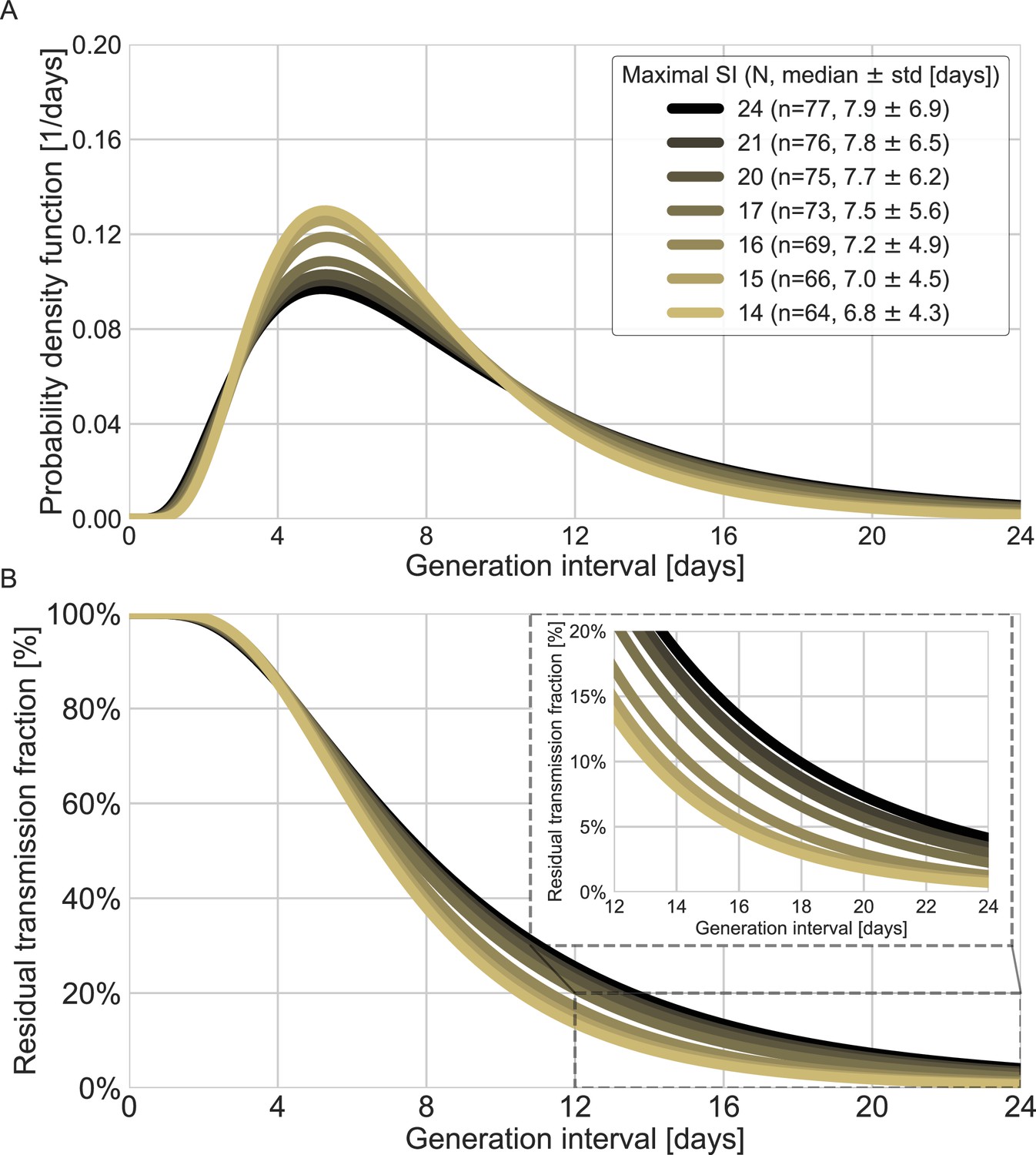
Sensitivity analysis to the top values of serial intervals.
The generation-interval distribution is inferred by maximum likelihood when the transmission pairs with the highest serial intervals are removed. (A) The probability density functions of the distributions. The legend reports the median and standard deviation of each of the distributions, as well as the number of transmission pairs remaining in the dataset after the removal of serial intervals exceeding the specified value. (B) The survival function of the generation-interval distribution, defined as the complement of the cumulative distribution, representing the residual fraction of transmission after a designated time since infection. The inset shows a zoom-in on the period of 12–24 days after exposure, a period in which there is a substantial difference between the current estimate and those from previous studies.
Figure 6 with 2 supplements
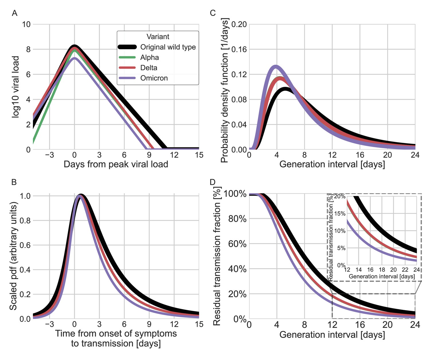
Using viral load trajectory for modeling other variants of concern (VOCs).
(A) The mean viral load trajectory for the main VOCs according to Kissler et al. (alpha and delta) and Hay et al. (delta and omicron). (B) Infectiousness profiles as derived from the probability density functions of the time from onset of symptoms to transmission (TOST) distribution (scaled to their maximal values). The black curve was derived for the original Wuhan variant (assumed to be close to non-VOCs in Kissler et al. study) using a maximum likelihood inference. The profiles for the alpha, delta, and omicron variants were estimated by scaling the time of the distribution by the ratio of the clearance’s durations. (C) The probability density function of the generation-interval distribution extrapolated for the various variants. (D) The survival function of the generation-interval distribution extrapolated for the various variants. The inset shows a zoom-in on the period of 12–24 days after exposure. The extrapolated distributions for the alpha and delta variants are extremely close, hence the green line is hidden by the red line in panels B–D.
Figure 6—figure supplement 1
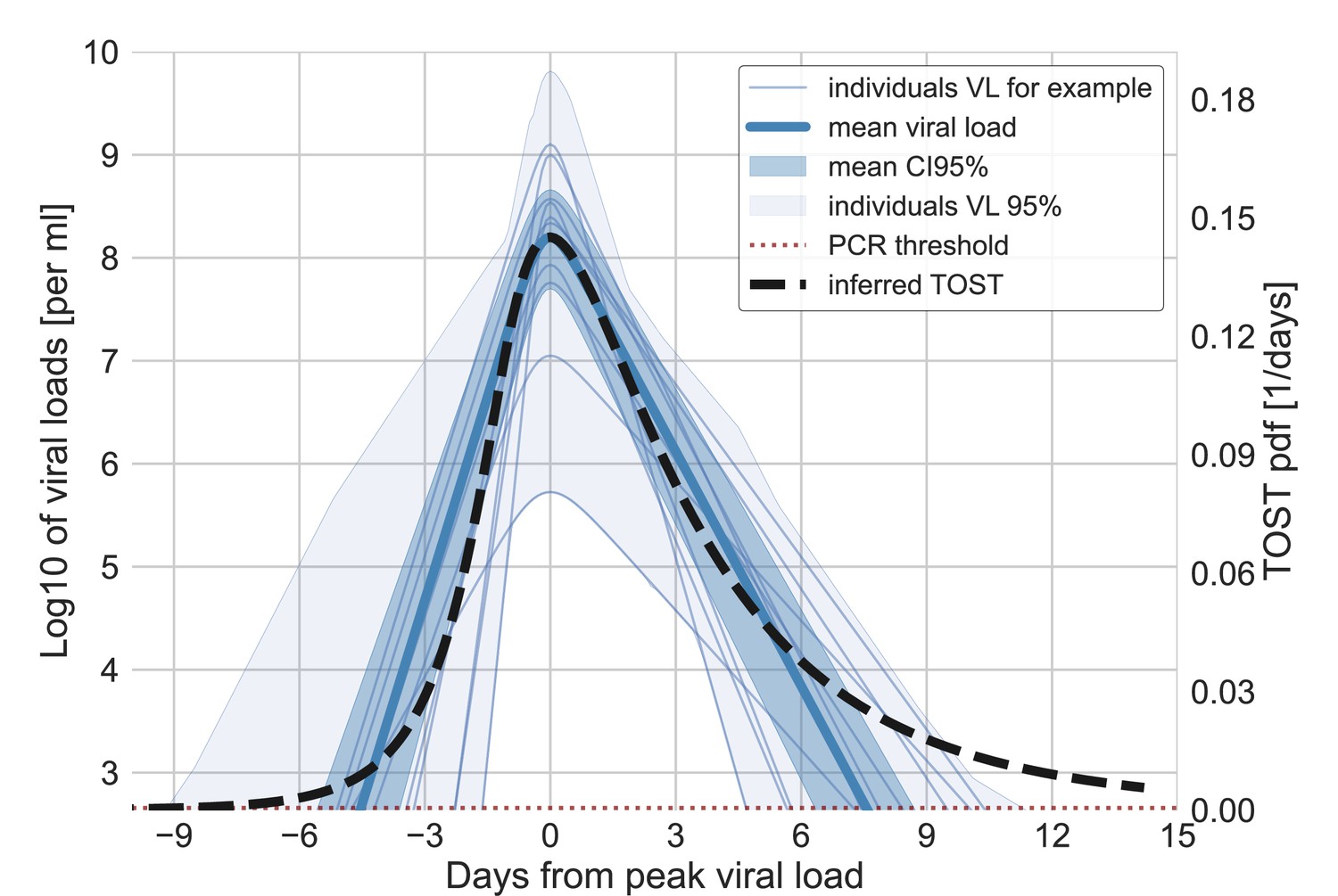
Variability of the viral loads and the potential connection with inferred infectiousness.
Examples for 10 individual viral load trajectories inferred by Kissler et al. for non-variant of concern (VOC) patients, together with the statistics of the variation of the inferred trajectories of all 41 individuals (Kissler et al., 2021). The inferred mean viral load trajectory is also shown together with its 95% credible interval. The viral loads are presented on a scale with a minimum that corresponds to the detection limit of PCR. On the right y-axis, the TOST (time from symptoms onset to transmission) distribution is drawn such that its maxima coincides with the maximum of the mean viral load.
Figure 6—figure supplement 2
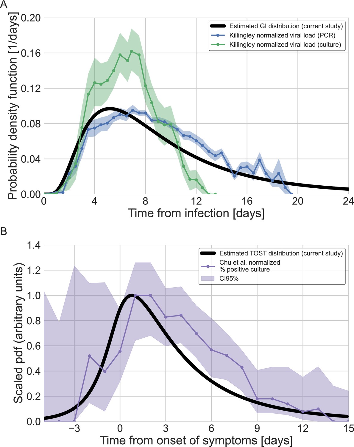
Comparison of estimated infectiousness profile with viral loads and positive culture data.
(A) The estimated generation-interval distribution is compared to viral loads that was measured from 18 individuals in a challenge trial (Killingley et al., 2022). The viral loads were measured from the day of inoculation and normalized to represent a density distribution (integral of one). The dots present the mean of the measurements and the shaded represent one standard error of the mean. (B) The estimated TOST (time from symptoms onset to transmission) is compared to the fraction of positive culture, measured as a function of time since symptoms onset for over 200 patients taken from Chu et al., 2022. Both the TOST distribution and the fraction of positive culture are normalized to have a maximum of one.
Appendix 1—figure 1
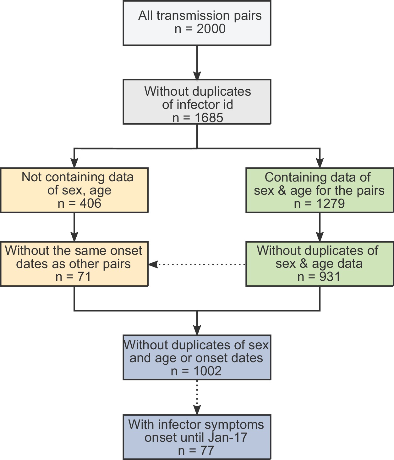
The obtained dataset of transmission pairs.
The merged datasets were filtered to remove duplicates in three stages: first removal of transmission pairs with the same infector and infectee ID. Second, identification of duplicates sharing the same symptom-onset dates as well as sex and age information. Lastly, transmission pairs without sex and age information were added only if their symptom-onset dates did not already occur in the dataset.
Appendix 1—figure 2
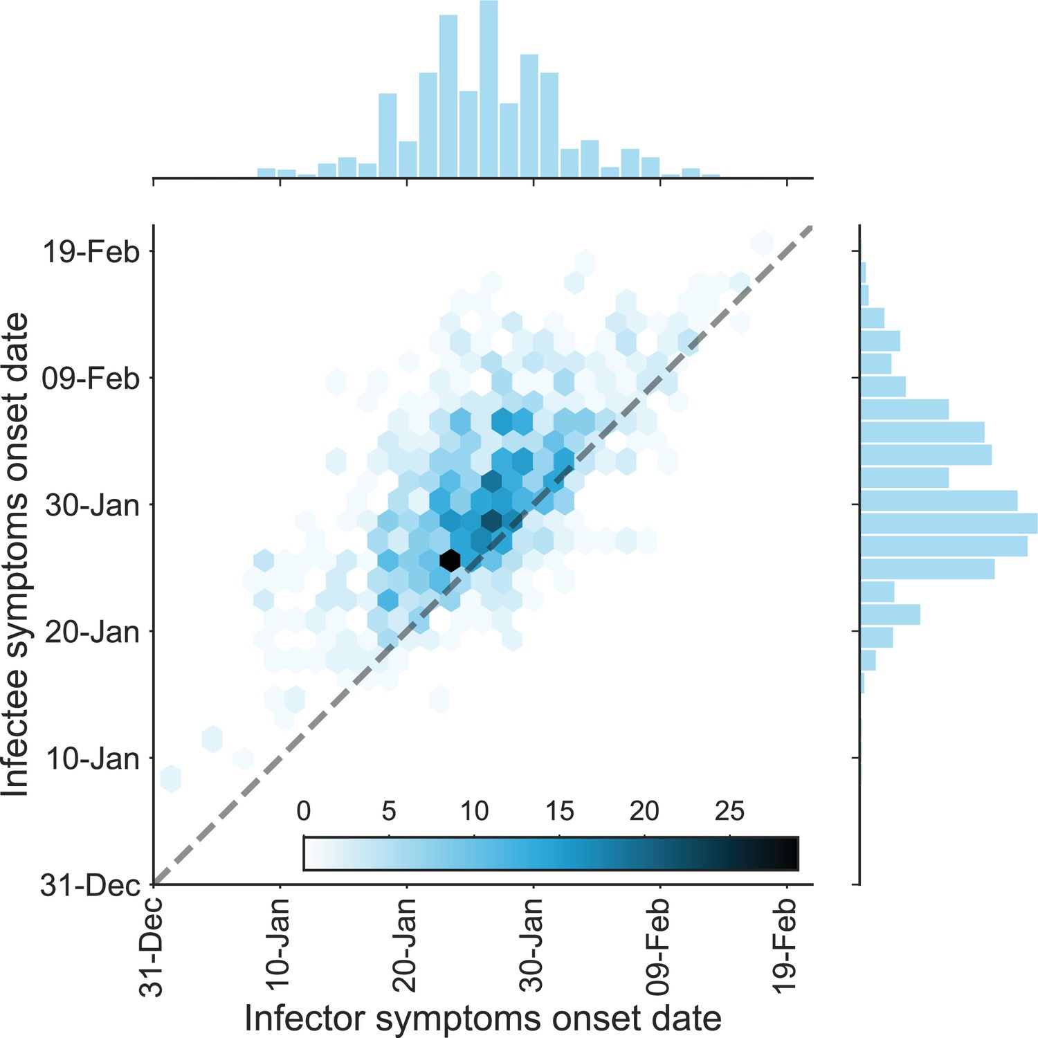
The dataset of transmission pairs – infectee symptoms onset date vs. infector symptoms onset date.
The observed bivariate distribution of time of symptoms development is shown via a hexbin graph. The plane is divided into hexagons that are colored according to the number of data points in the dataset they represent. The marginal empirical distributions are shown using a histogram on the sides. The dotted line represents data points for which the symptoms’ onset date of the infector is the same as that of the infectee.
Appendix 1—figure 3
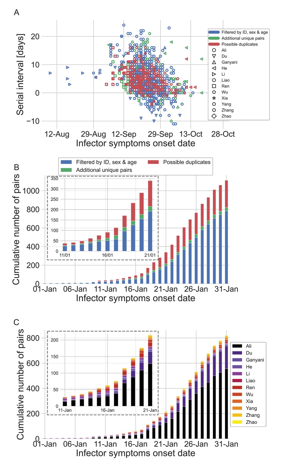
The dataset of transmission pairs as a function of the infector symptoms onset date.
(A) Scatter plot of serial intervals plotted against the symptoms onset date of the infector. The three levels of filtering are color-coded, while the shape of the marker represents the reference from which the data was taken. (B) The cumulative number of cases as a function of the infector symptoms onset date, where the data is divided between the three levels of filtration. The inset focuses on the period that at its end interventions were made. (C) The cumulative number of cases as a function of the infector symptoms onset date, where the data is divided between the data sources. The dataset is shown after filtrating by ID, sex, and age and the addition of unique pairs (no duplicates). The inset focuses on the period that at its end interventions were made.
Appendix 1—figure 4
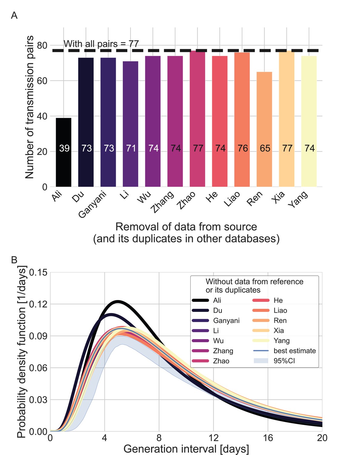
Sensitivity analysis regarding the inclusion of a dataset from a specific source.
Beginning with the complete dataset of transmission pairs with infector onset until January 17, 2020 (after filtering by ID, sex, and age and adding unique pairs, see Appendix 1—figure 1), partial datasets were created by omitting all transmission pairs from each source of data and all its duplicates in the other datasets. (A) The number of transmission pairs for each of the partial datasets, excluding pairs from a specific source dataset and their duplicates in other datasets. (B) Maximum likelihood estimates of the bivariate incubation period and generation-interval distribution. The uncertainty range of the maximum likelihood estimate of the complete dataset is also shown for comparison.
Appendix 1—figure 5
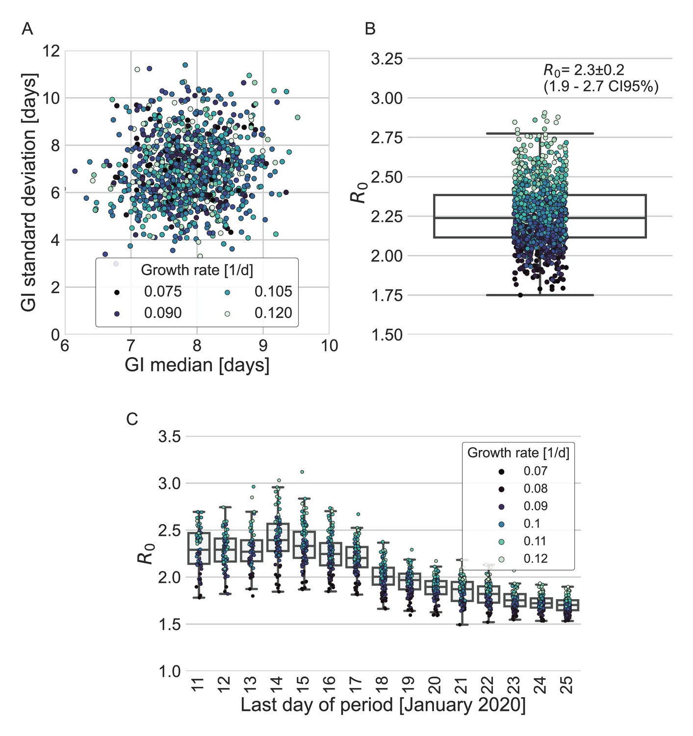
Estimates of R0 based on the inferred generation-interval distribution.
(A–B) Bootstrapping results of the parameters of the generation-interval distribution and the resulting estimates for R0. In the process of bootstrapping, the dataset of 77 transmission pairs was resampled with returns. In addition, the growth rate (r) was sampled from the distribution found in a recent study (Tsang et al., 2020). (A) Estimates of the mean and standard deviation of the generation interval. Each point represents the maximum likelihood estimate for a single run in a bootstrap process. The point was colored according to the sampled growth rate. (B) The distribution of estimates of R0 derived from the generation-interval distribution and growth rate. The box represents the interquartile range (percentiles 25–75) and the whiskers represent the maximal range of the distribution apart from outliers (defined as data points exceeding the interquartile range by a factor of 1.5). The mean (with its 95% confidence interval) and the standard deviation is given in the legend. The points are colored according to the sample growth rate, as in panel A. (C) The dependence of R0 estimates on the period taken in the analysis. The boxes represent the interquartile range (percentiles 25–75) and the whiskers represent the maximal range of the distribution apart from outliers (defined as data points exceeding the interquartile range by a factor of 1.5). The points are colored according to the sample growth rate, as described in the legend.
Appendix 1—figure 6
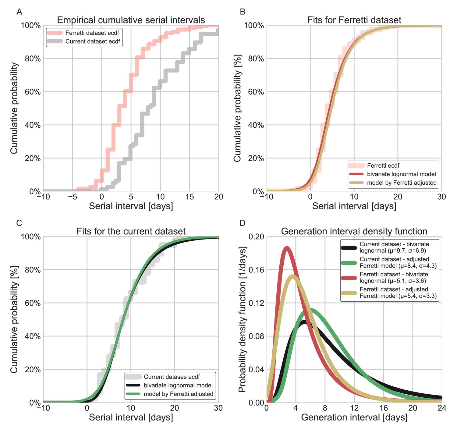
Comparison of the current dataset and model with that of Ferretti et al., 2020a.
The maximum likelihood framework was used to fit both the current dataset and the one provided in the Figure 1 of Ferretti et al. The datasets were fit using either the lognormal bivariate model described in the Methods section, or a reconstructed model following Ferretti et al., 2020a, adjusted by adding a parameter for shifting the time from onset of symptoms to transmission (TOST) function over the x-axis. (A) The empirical cumulative distribution of serial intervals, comparison between the dataset of Ferretti et al., 2020a, and the current dataset curated in this study. (B) Maximum likelihood fits for the dataset provided in Figure 1 of Ferretti et al. (C) Maximum likelihood fits for the current dataset. (D) The marginal generation-interval distributions of the maximum likelihood fits. The mean and standard deviation are provided in the legend.
Appendix 1—figure 7
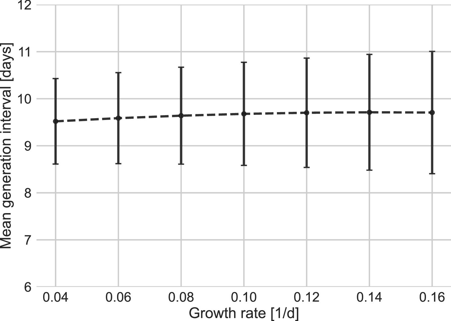
Sensitivity analysis to the growth rate.
The mean of the generation-interval distributions were estimated using the maximum likelihood fits for the dataset with growth rates in the range of 0.04–0.16 day–1. Estimates of the uncertainty were obtained using bootstrapping (30 runs for each value of r). Error bars represent 95% confidence interval.
Appendix 1—figure 8
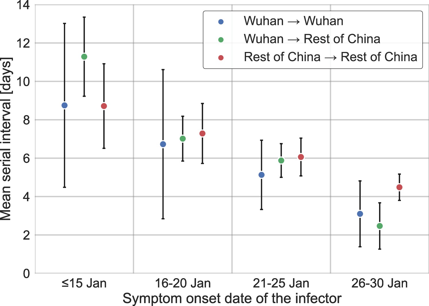
Stratification of the serial interval data by the location of infection.
A comparison of the mean of the observed distribution of serial intervals divided to four time periods of the infector symptom onset, and stratified by the infection location of the infector and infectee. Error bars represent 95% confidence interval.
Appendix 1—figure 9
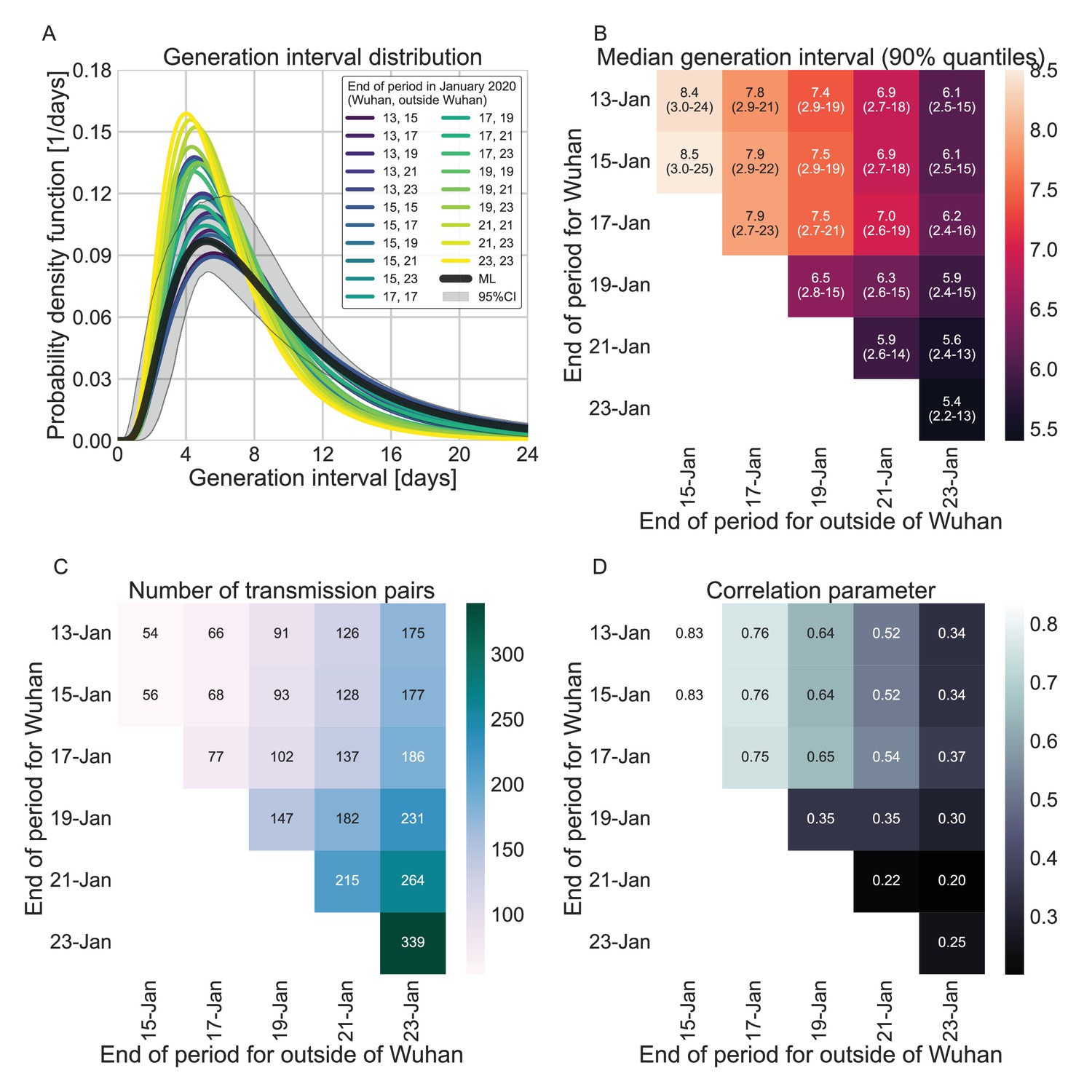
Sensitivity analysis to the definition of the period of interest for infectors that were infected in or outside Wuhan.
A comparison of the resulting maximum likelihood estimates where the period of interest was defined separately for infectors who were infected in or outside of Wuhan. (A) The shapes of the resulting generation-interval distribution. For comparison, the main analysis’ maximum likelihood is presented together with its 95% interval (the highlighted area). (B) Estimates of the median generation intervals and the 90% interquartile range as function of the period of interest, defined separately for infectors who were infected in or outside of Wuhan. (C) Number of transmission pairs analyzed as function of the period of interest, defined separately for infectors who were infected in or outside of Wuhan. (D) Estimates for the correlation between incubation period and generation-interval parameter as function of the period of interest, defined separately for infectors who were infected in or outside of Wuhan.
Appendix 1—figure 10

Sensitivity analysis to the assumed incubation period distribution.
The generation-interval distribution is inferred by maximum likelihood when the incubation period distribution is assumed to have a different median (scale parameter). (A) The probability density functions of the incubation distributions taken in the sensitivity analysis, corresponding medians of 4, 4.5, 5, and 5.5 days. (B) The resulting probability density function of the generation intervals. Legend reports the median and standard deviation of each of the distributions.
Appendix 1—figure 11
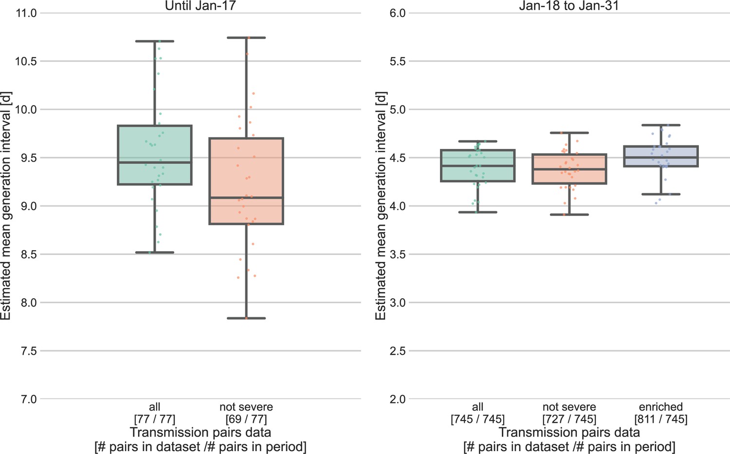
Sensitivity analysis for the severity of cases.
Severe cases (including death) are over-represented in the period prior to January 17, with 8 out of 77 cases, compared to 18 out of 745 in the period of January 18–31. The effect of inclusion of severe cases was analyzed by comparing the means of the estimated generation-interval distribution, separately for the two periods in question, using the inference framework with 30 bootstrapping runs. For the earlier period, the estimated mean were compared for the dataset with or without the severe cases. For the later period, we also compared the results to an enriched dataset in which the severe cases were oversampled (using bootstrapping) such that the proportion of severe cases matches that during the earlier period (10%). The boxes represent the interquartile range (percentiles 25–75) and the whiskers represent the maximal range of the distribution apart from outliers (defined as data points exceeding the interquartile range by a factor of 1.5).
Appendix 1—figure 12
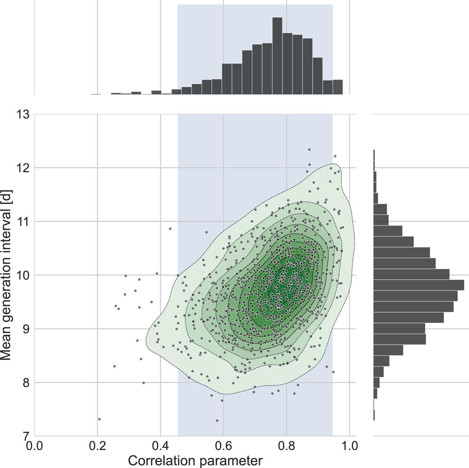
The connection between the estimated mean generation interval and the correlation parameter.
One thousand bootstrap runs were conducted for estimation of the uncertainty of the inferred bivariate distribution of incubation period and generation interval. The mean of the generation-interval distribution was derived and plotted against the estimated correlation parameter for each run together with contours representing quantiles of equal probability (central panel). The margin distributions of the two parameters are shown on the right and upper panel. The shaded region corresponds to the 95% confidence interval of the correlation parameter (0.45–0.95).
Appendix 1—figure 13
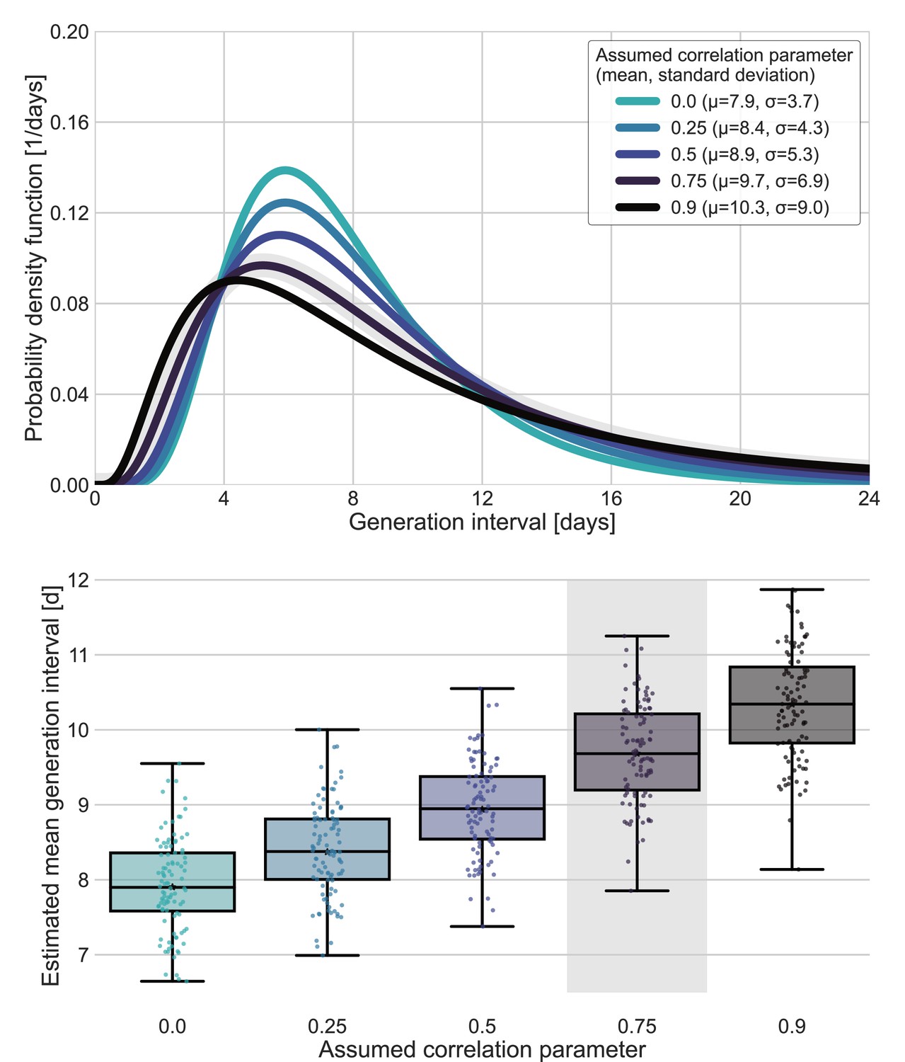
Sensitivity analysis for fixed correlation parameters.
Maximum likelihood estimates of the bivariate incubation period and generation-interval distribution were made for datasets containing the transmission pairs with infector onset date up January 17 while the correlation parameter was fixed at one of 0, 0.25, 0.5, 0.75, 0.9. Best estimates were derived for each of the datasets. Uncertainty estimates were derived by bootstrapping, through sampling with replacement from the dataset and sampling from the distribution of growth rates (Tsang et al., 2020) N=100 times. (A) Best estimate for the generation-interval distribution probability density function for assumed correlation parameters. (B) Best estimates and distributions of the mean generation interval. A black star marks best estimates. Ranges are given as boxplots. The box represents the interquartile range (percentiles 25–75) and the whiskers represent the maximal range of the distribution apart from outliers (defined as data points exceeding the interquartile range by a factor of 1.5). The fitted correlation (0.75) is highlighted in gray shade.
Tables
Table 1
The main biases of infectiousness profile inference from serial-interval data discussed in the Introduction section.
| Source of bias | Expected net effect on the inferred generation-interval distribution | Current study’s approach for correcting the bias | Studies who considered this bias |
|---|---|---|---|
| Mitigation steps and awareness limit the spread of the disease | Underestimation of the mean generation interval | Curation of cases focus only on early spread | – |
| Realized serial intervals depends on the rate of the spread of the disease | Systematic difference between serial- and generation-interval distributions | Correction for backward incubation period distribution | Park et al., 2021; Ferretti et al., 2020b |
| Possible correlation of incubation periods and temporal profile of infectiousness | Underestimation of the mean generation interval | Modeling infectiousness using incubation period and generation-interval bivariate distribution | Hart et al., 2021; Ferretti et al., 2020a |
Additional files
-
Supplementary file 1
The combined dataset of transmission pairs from the early spread of the COVID-19 epidemic in China.
- https://cdn.elifesciences.org/articles/79134/elife-79134-supp1-v2.csv
-
MDAR checklist
- https://cdn.elifesciences.org/articles/79134/elife-79134-mdarchecklist1-v2.docx
Download links
A two-part list of links to download the article, or parts of the article, in various formats.
Downloads (link to download the article as PDF)
Open citations (links to open the citations from this article in various online reference manager services)
Cite this article (links to download the citations from this article in formats compatible with various reference manager tools)
The unmitigated profile of COVID-19 infectiousness
eLife 11:e79134.
https://doi.org/10.7554/eLife.79134


