Deep mutational scanning and machine learning reveal structural and molecular rules governing allosteric hotspots in homologous proteins
- Department of Biochemistry, University of Wisconsin-Madison, United States
- Department of Physics, Boston University, United States
- Department of Chemistry, Boston University, United States
- Department of Bacteriology, University of Wisconsin-Madison, United States
- Department of Chemical and Biological Engineering, University of Wisconsin-Madison, United States
Figures
Figure 1 with 7 supplements
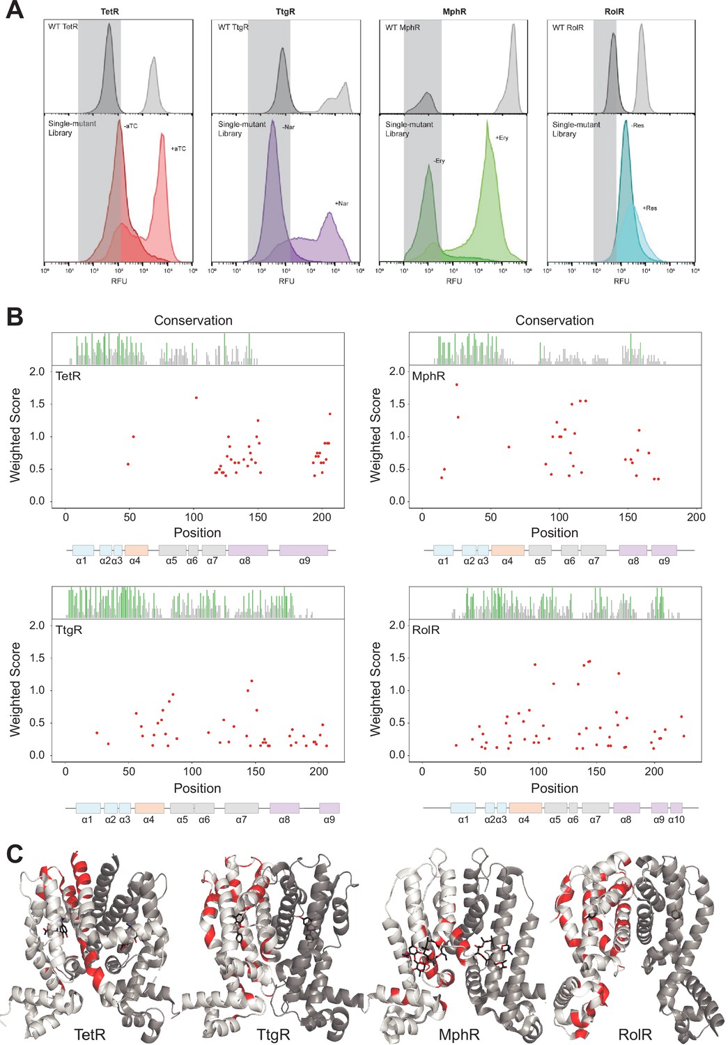
Allosteric hotspots in four bacterial allosteric transcription factors (aTFs) identified using deep mutational scanning (DMS).
(A) Nonfluorescent cells in the TetR, TtgR, MphR, and RolR single-mutant library were sorted (gray bar) in the presence (light shade) and absence (dark shade) of 1 µM anhydrotetracycline (aTC), 500 µM naringenin (Nar), 1 mM erythromycin (Ery), and 7.5 mM resorcinol (Res), respectively, and sequenced to identify dead variants. Sorting gates were defined by the wild-type uninduced population for each homolog. (B) Allosteric hotspots (red points) for each aTF is shown with residue numbers along x axis and a weighted score along y axis based on the number of dead mutations at a residue position. Secondary structures of the aTFs are illustrated below and colored according to regions (blue: DBD, orange: hinge helix connecting LBD and DBD, gray: LBD and purple: dimer interface). Residue conservation is shown and colored by conserved residues (green), not conserved (gray) and conserved overlapping with hotspot (red). (C) Allosteric hotspots mapped on to the structure of TetR, TtgR, MphR, and RolR (ligand-contacting residues excluded).
Figure 1—figure supplement 1
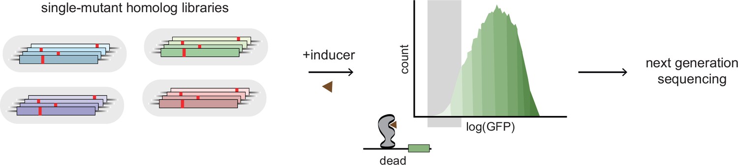
Experimental scheme for deep mutational scanning.
Protein-wide, single-site saturation mutagenesis of four TetR-like family allosteric transcription factors (aTFs) – TetR, TtgR, RolR, and MphR – using reporter-based screening followed by deep sequencing.
Figure 1—figure supplement 2
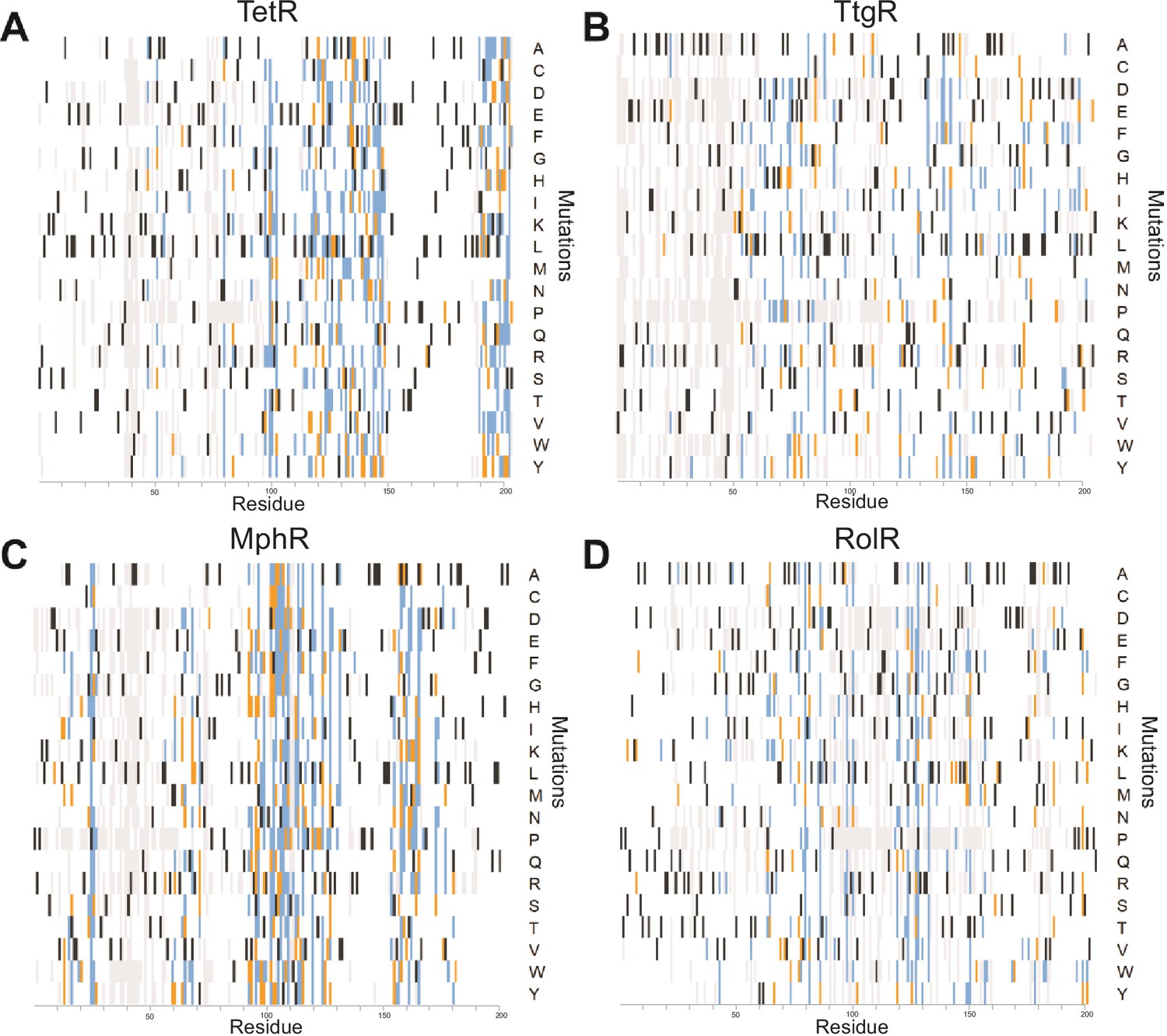
A detailed summary of all single-mutant phenotypes for every position within the proteins.
Heatmaps detailing the effect of all single mutants at every position in (A) TetR, (B) TtgR, (C) MphR, and (D) RolR are shown. Wild-type residues are black, mutations that do not affect protein function are white, mutants classified as dead in two or all three replicates are orange and blue, respectively. Variants not present in the dataset are gray.
Figure 1—figure supplement 3
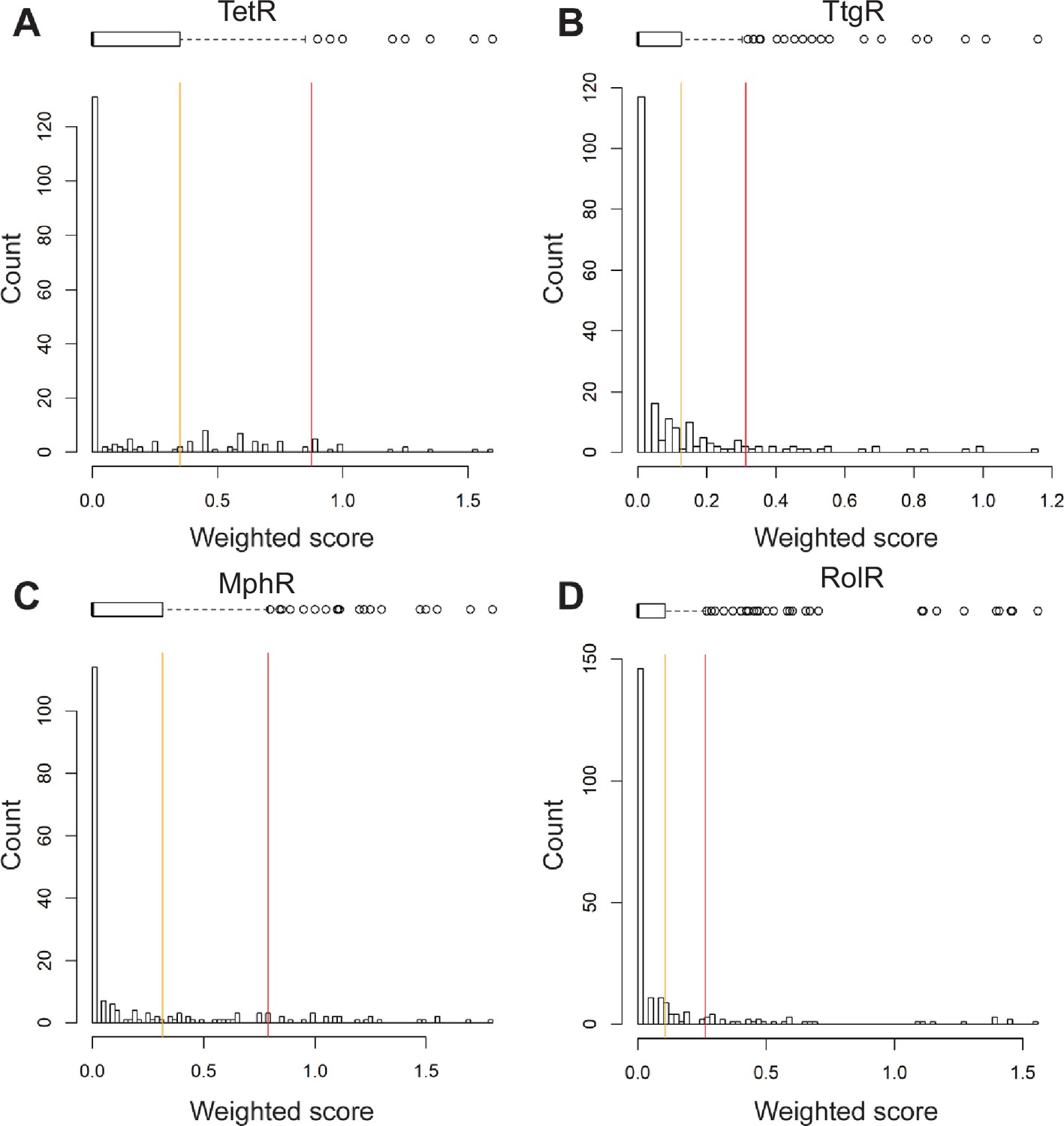
Histograms of weighted scores and thresholds for identifying hotspots.
The distribution of weighted scores for every position in (A) TetR, (B) TtgR, (C) MphR, and (D) RolR is shown. Box and whisker plots above each histogram illustrate the spread of the data where outliers are shown as circles (red line) and all positions above Q3 (orange line) were designated allosteric hotspots.
Figure 1—figure supplement 4
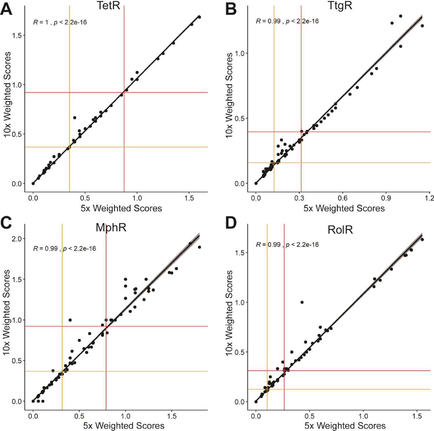
Correlation of weighted scores between a ×5 or ×10 read count threshold.
The correlation of weighted scores for every position using a ×5 or ×10 read count threshold is shown for (A) TetR, (B) TtgR, (C) MphR, and (D) RolR. The red and orange lines illustrate the spread of the data using interquartile range where outliers are plotted above the red line and all positions in the top quartile are designated allosteric hotspots.
Figure 1—figure supplement 5
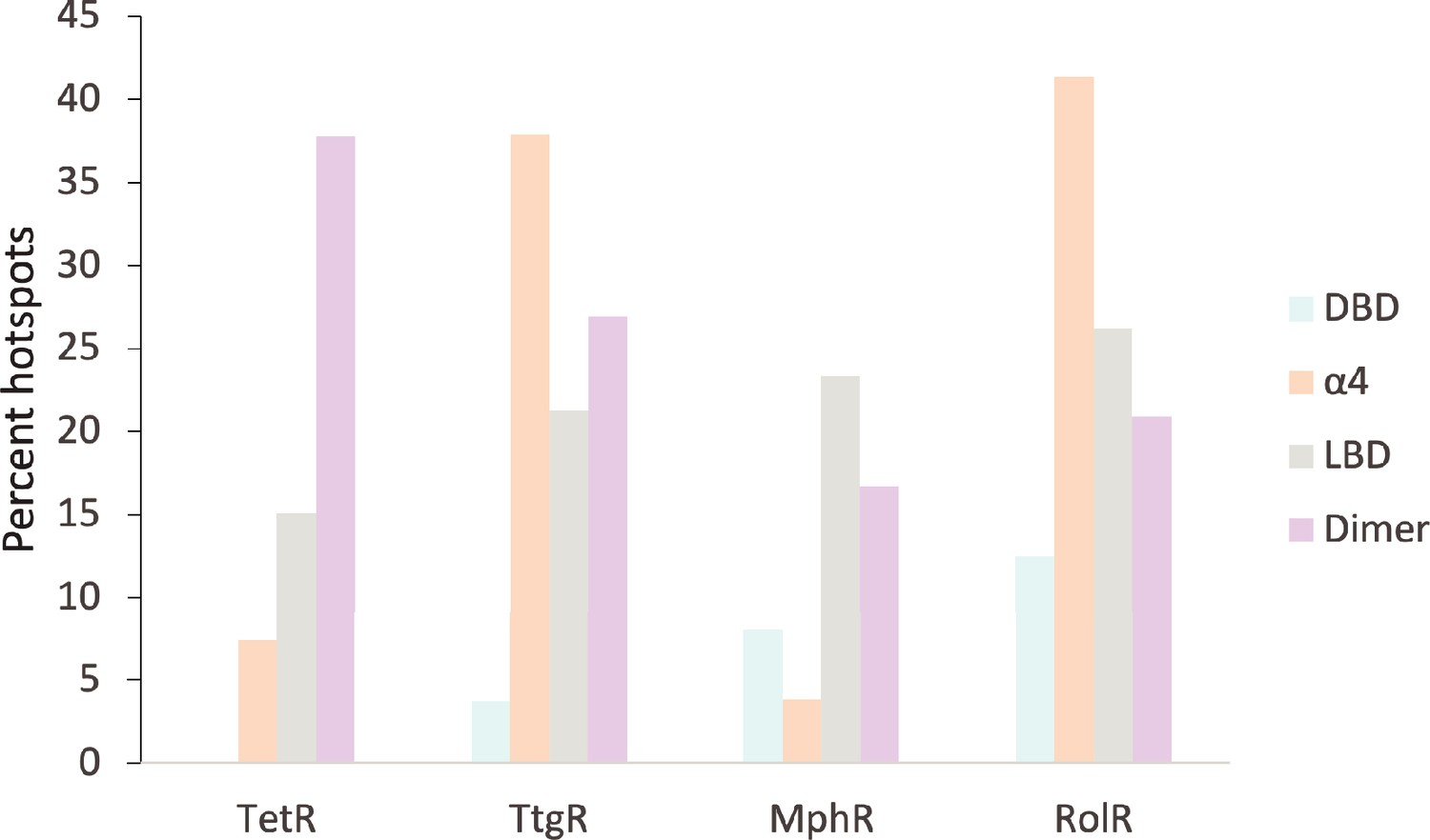
Distribution of allosteric hotspots in TetR homologs.
The percent of hotspots in the four main structural regions of the TetR homologs. Regions were broken into groups based on the crystal structures of TetR (PDB ID: 4AC0), TtgR (PDB ID: 2UXU), MphR (PDB ID: 3FRQ), and RolR (PDB ID: 3AQT). Potential ligand-binding residues are included in the statistics but are not considered hotspots.
Figure 1—figure supplement 6
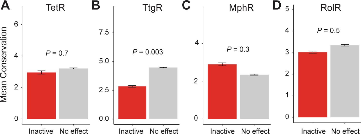
Conservation of allosteric hotspots.
Average conservation score of all positions considered inactive or having no effect in (A) TetR, (B) TtgR, (C) MphR, and (D) RolR. Data show as mean ± SEM.
Figure 1—figure supplement 7
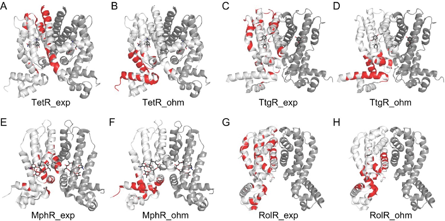
Comparison of experimental hotspots with predictions made by the Ohm server.
Allosteric hotspots of TetR, TtgR, MphR, and RolR determined by experiments (A, C, E, G) and the Ohm webserver (B, D, F, H) differ significantly. The Ohm webserver identifies critical residues along the signal propagation pathways between the bound effectors (ligands) to the active sites (DNA-binding residues) as allosteric hotspots. Specifically, in the Ohm calculation, signals are started from effector molecules, which are then propagated through residue contacts, with the active sites as signal sinks. Such signal propagation simulation is repeated for 104 times, and the residues that appear most frequently in pathways connecting effectors and active sites are recognized as hotspots. The number of hotspots identified by Ohm calculation is made equal to experimentally determined hotspots. The accuracy of hotspot identification of Ohm calculation is 0.08 for TetR; 0.12 for TtgR; 0.31 for MphR, and 0.40 for RolR.
Figure 2 with 2 supplements
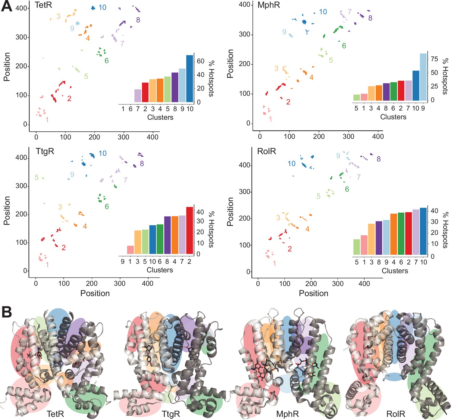
Hotspots enriched among long-range interactions (LRIs).
(A) Residue-residue contact map showing LRIs within each homolog. The LRIs are grouped by color, following standard k-means clustering, representing different regions of the protein. Inset shows ranking of LRI clusters based on the percentage of unique hotspots within each cluster. (B) The general location of each LRI cluster on the protein structure (color scheme same as panel A).
Figure 2—figure supplement 1
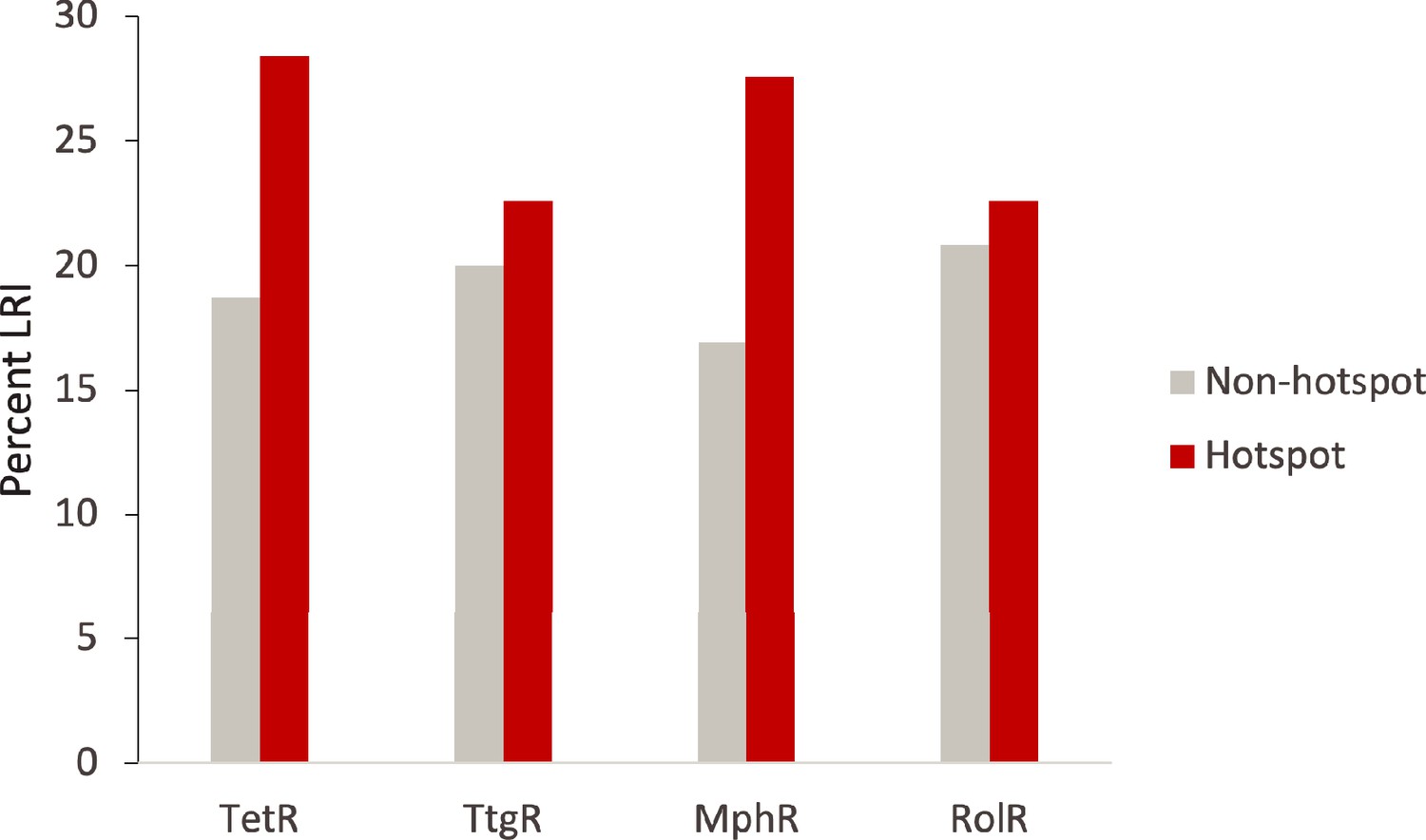
Hotspot interactions are more likely to be long range than those of non-hotspots.
The percent of hotspot and non-hotspot residues participating in long-range interactions (LRIs) in each homolog protein.
Figure 2—figure supplement 2
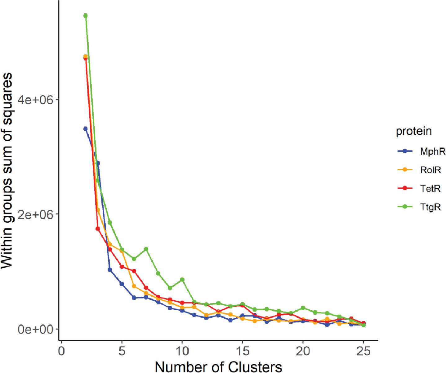
Elbow method to determine the optimal number of clusters.
The optimal number of clusters to use for the k-means clustering of long-range interactions (LRIs) in each homolog was determined by iteratively calculating the variance within clusters for 1–25 clusters.
Figure 3 with 1 supplement
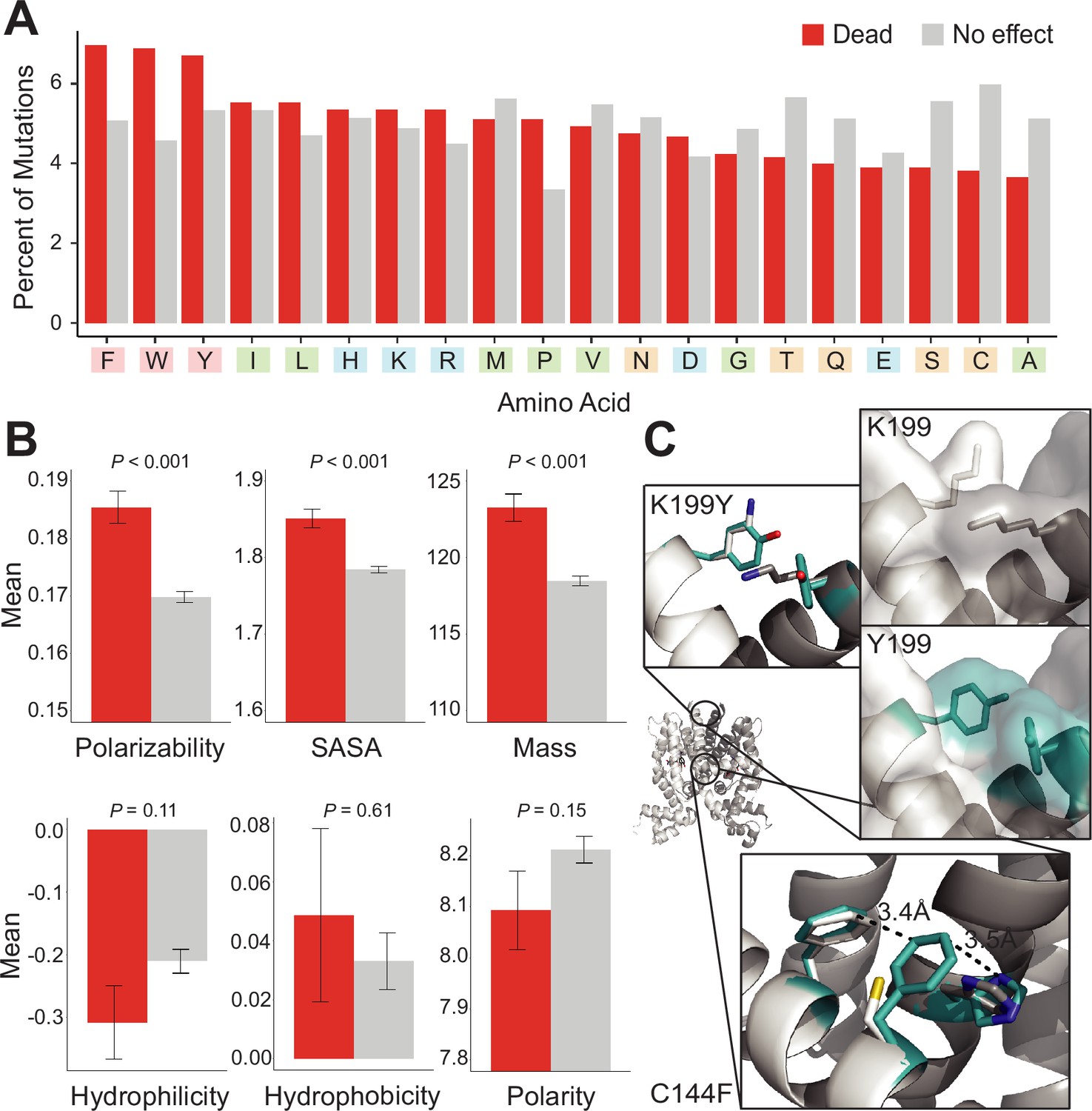
Mutational preferences and physicochemical properties of dead variants.
(A) Percentage of mutations (final mutated state) among dead (red) and not-dead (gray) variants from deep mutational scanning (DMS) data for all four homologs combined. (B) Comparison of physicochemical properties – polarizability, solvent-accessible surface area (SASA), mass, hydrophilicity, hydrophobicity, and polarity – between dead (red) and not-dead variants (gray). Average values aggregated over all four DMS datasets shown. Data represented as mean ± SEM. (C) Structural models of the K199Y (top) and C144F (bottom) mutations in TetR. Residues in the mutant structures are colored teal and the two monomers are colored white and dark gray.
Figure 3—figure supplement 1
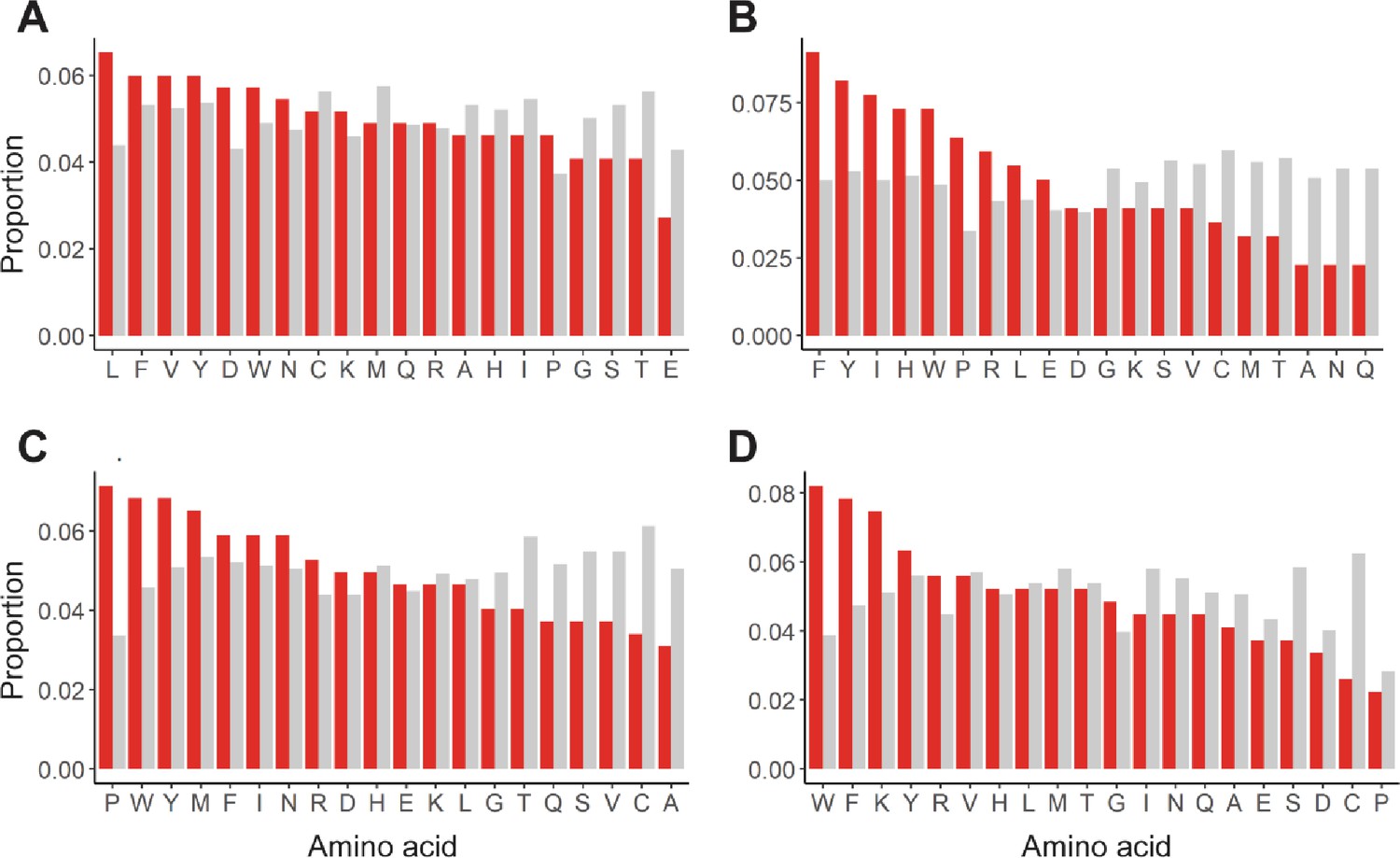
Enrichment of mutations in allosterically dead or no effect variants.
Mutations in (A) TetR, (B) TtgR, (C) MphR, and (D) RolR were separated based on their effect on protein function, dead (red) or no effect (gray), and the proportion of each of the 20 amino acids within each set calculated to identify enrichments in allosterically dead or neutral variants.
Figure 4 with 8 supplements
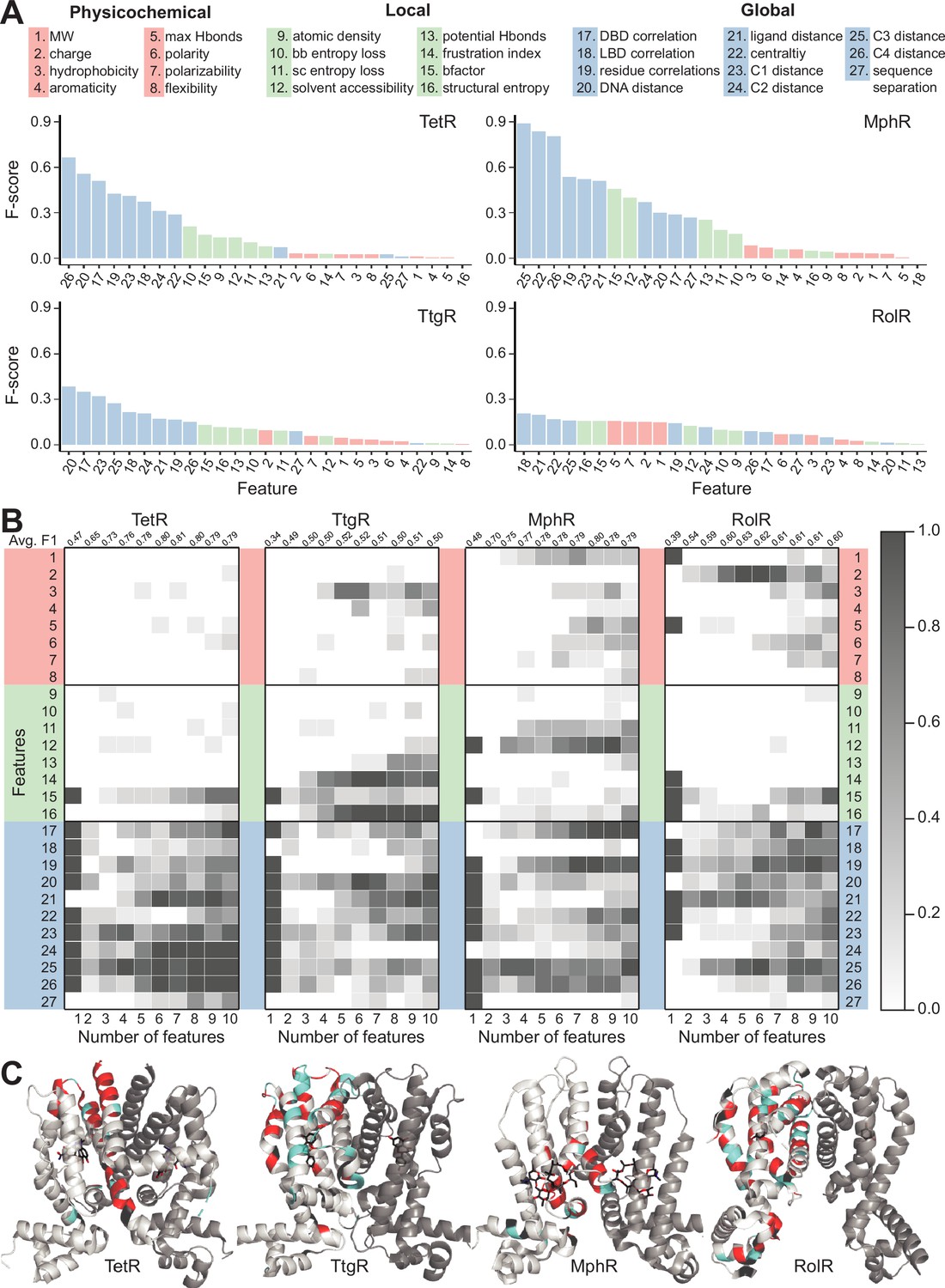
Machine learning identifies structural and molecular features that differentiate allosteric hotspots.
(A) The full list of 27 features is shown at the top. The F scores (measure of importance) of the features for each of the four allosteric transcription factors (aTFs) is shown below. (B) Frequency of appearance of the 27 features in the top ten 1–10 feature combinations ranked by F1 score for each protein. Row 2–28 corresponds to feature 1–27, row 1 is the average F1 score of the top ten 1–10 feature combinations. (C) Predictions made by the model based on the best fivefold cross-validation performance achieved for each aTF (red: true positive; cyan: false positive; black: false negative; rest: true negative). The features used in the best models are 2, 19, 21, 23–26 for TetR; 4, 7, 10, 15, 19, 21, 24, 25 for MphR; 2, 10, 12, 21, 25 for RolR, and 9, 10, 13, 23, 25 for TtgR.
Figure 4—figure supplement 1
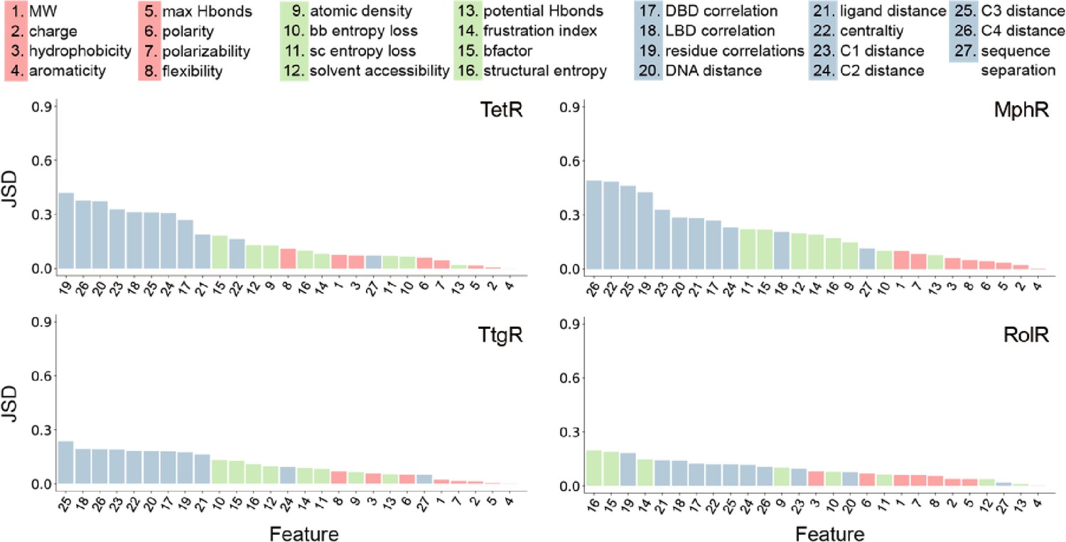
Global features have the highest Jensen-Shannon divergence (JSD).
The full list of 27 features is shown at the top. The JSDs (measure of importance) of the features for each of the four allosteric transcription factors (aTFs) is shown below. JSD is a measure of similarity between two probability distributions P and Q, which is bound between 0 (P and Q are the same) and 1 (P and Q have no overlap). The larger the JSD, the more different the two distributions are, and thus the features with larger JSDs are more discriminative for hotspot residues. JSD is a symmetrized and smoothed version of the more familiar Kullback-Liebler divergence defined as JSD(P||Q) = { DKL(P||M)+DKL(Q||M) }/2, where M = (P+Q)/2 is the average of two distributions and DKL is the Kullback-Liebler divergence (KL divergence) which also measures similarity between two distributions. KL divergence is defined as DKL(P||M) = ∑xP(x)*log2[P(x)/M(x)], x are points of the probability space where discrete distributions P and M are defined.
Figure 4—figure supplement 2
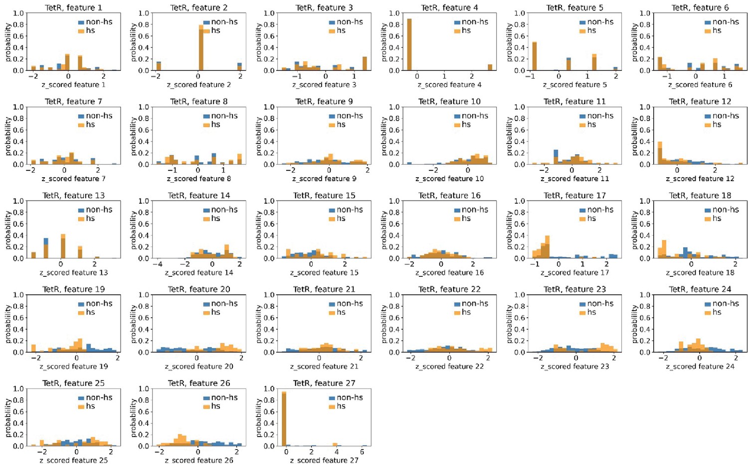
Distributions of TetR’s hotspots’ and non-hotspots’ z-scored feature values for feature 1–27.
The 27 plots correspond to the distributions of TetR’s hotspots’ (hs) and non-hotspots’ (non-hs) z-scored feature values for feature 1–27 as labeled by figure titles. The distributions of hotspots and non-hotspots are normalized by their populations, thus the y axis of the figures are probabilities. Z-scored feature j value of a residue n (Znj) is defined as the difference between its raw feature j value (Rnj) and the average raw feature j values of all residues (avg_Ri), divided by the standard deviation of raw feature j values of all residues, Znj = (Rnj - avg_Rj)/std_Rj.
Figure 4—figure supplement 3
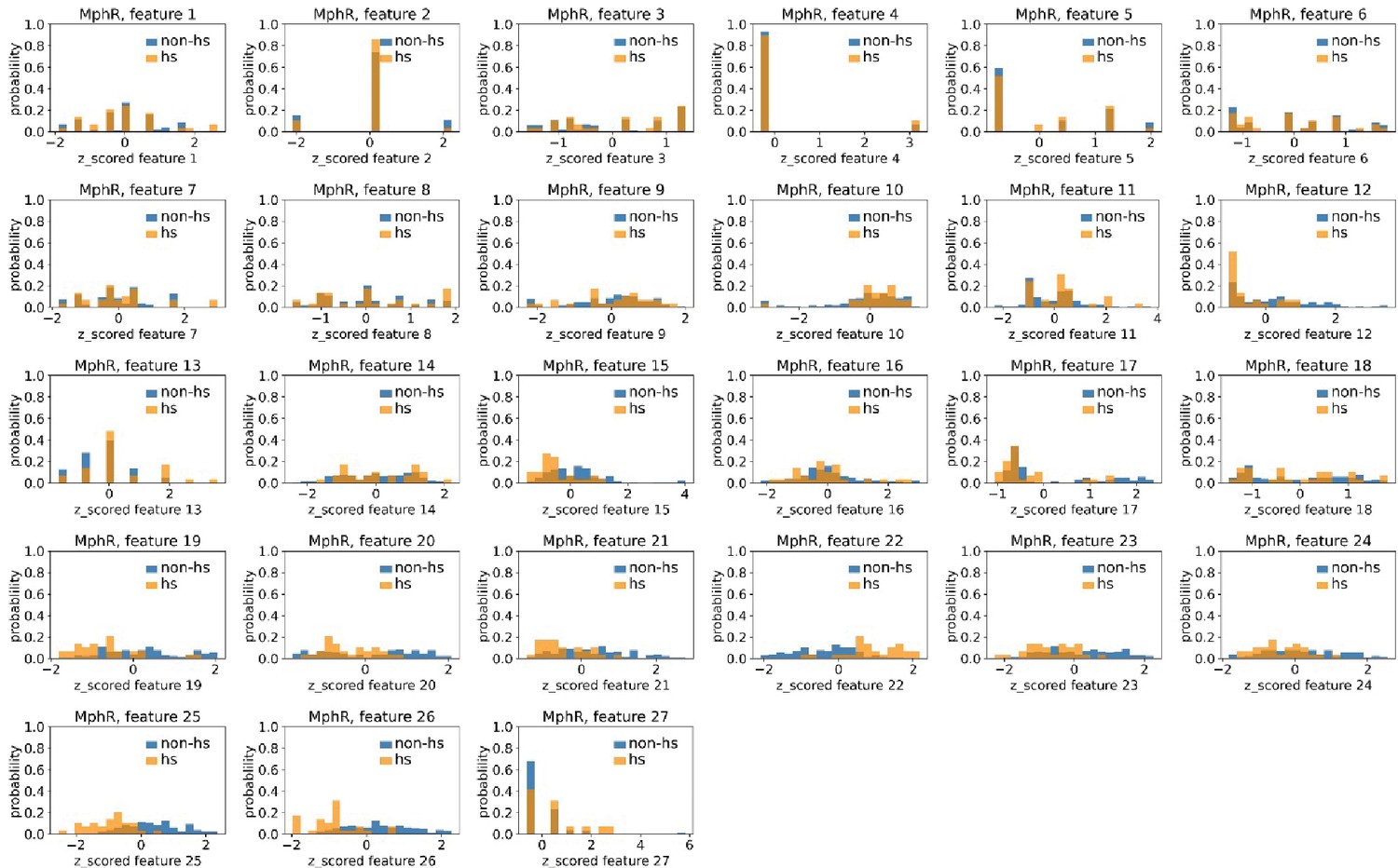
Distributions of MphR’s hotspots’ and non-hotspots’ z-scored feature values for feature 1–27.
The 27 plots correspond to the distributions of MphR’s hotspots’ (hs) and non-hotspots’ (non-hs) z-scored feature values for feature 1–27 as labeled by figure titles. The distributions of hotspots and non-hotspots are normalized by their populations, thus the y axis of the figures are probabilities. Z-scored feature j value of a residue n (Znj) is defined as the difference between its raw feature j value (Rnj) and the average raw feature j values of all residues (avg_Ri), divided by the standard deviation of raw feature j values of all residues, Znj = (Rnj − avg_Rj)/std_Rj.
Figure 4—figure supplement 4
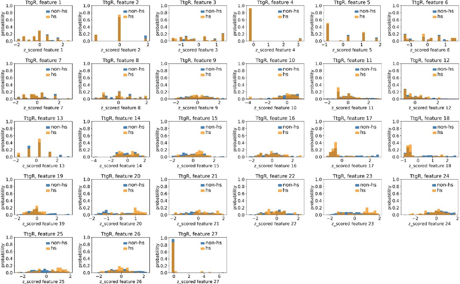
Distributions of TtgR’s hotspots’ and non-hotspots’ z-scored feature values for feature 1–27.
The 27 plots correspond to the distributions of TtgR’s hotspots’ (hs) and non-hotspots’ (non-hs) z-scored feature values for feature 1–27 as labeled by figure titles. The distributions of hotspots and non-hotspots are normalized by their populations, thus the y axis of the figures are probabilities. Z-scored feature j value of a residue n (Znj) is defined as the difference between its raw feature j value (Rnj) and the average raw feature j values of all residues (avg_Ri), divided by the standard deviation of raw feature j values of all residues, Znj = (Rnj − avg_Rj)/std_Rj.
Figure 4—figure supplement 5
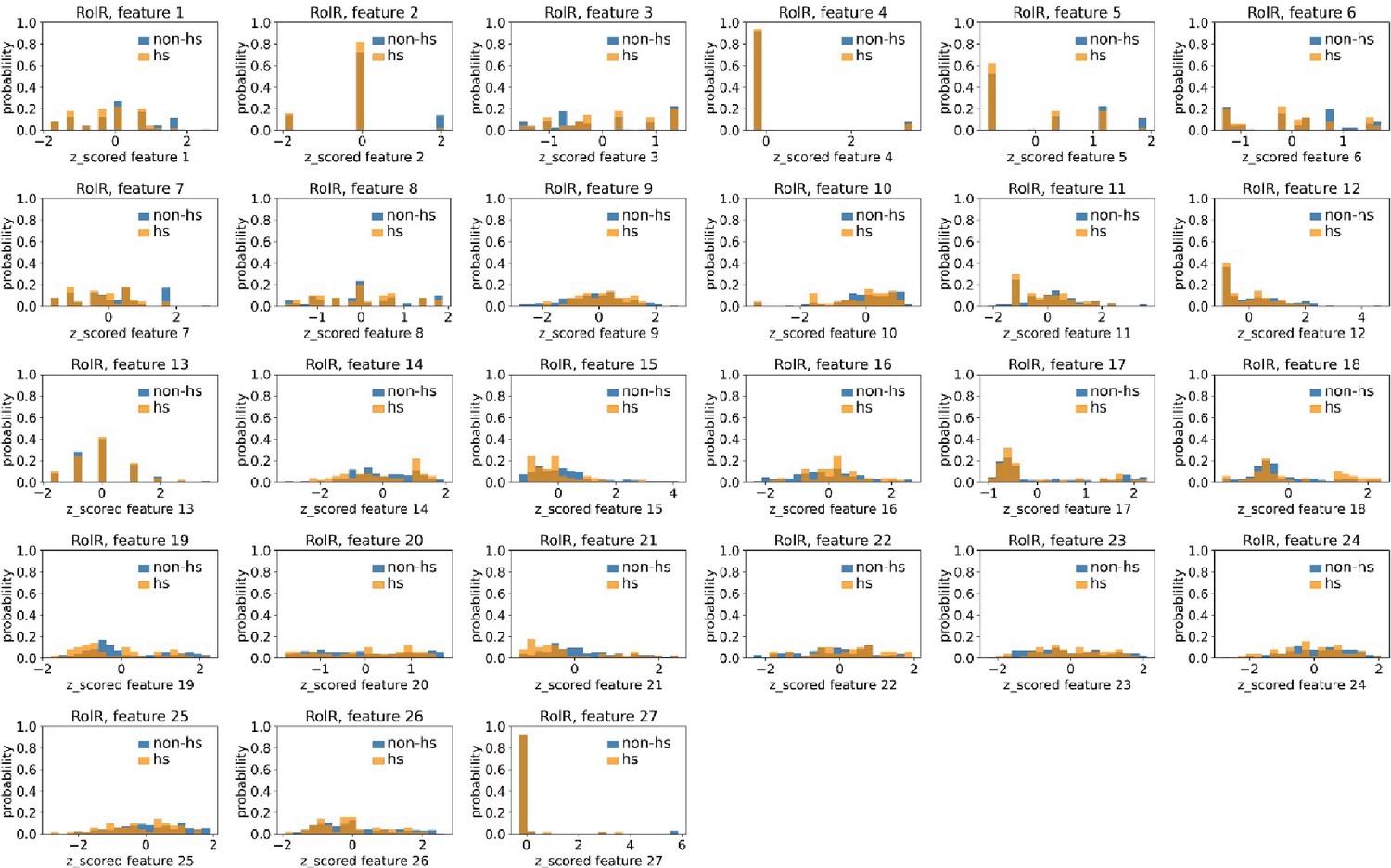
Distributions of RolR’s hotspots’ and non-hotspots’ z-scored feature values for feature 1–27.
The 27 plots correspond to the distributions of RolR’s hotspots’ (hs) and non-hotspots’ (non-hs) z-scored feature values for feature 1–27 as labeled by figure titles. The distributions of hotspots and non-hotspots are normalized by their populations, thus the y axis of the figures are probabilities. Z-scored feature j value of a residue n (Znj) is defined as the difference between its raw feature j value (Rnj) and the average raw feature j values of all residues (avg_Ri), divided by the standard deviation of raw feature j values of all residues, Znj = (Rnj − avg_Rj)/std_Rj.
Figure 4—figure supplement 6
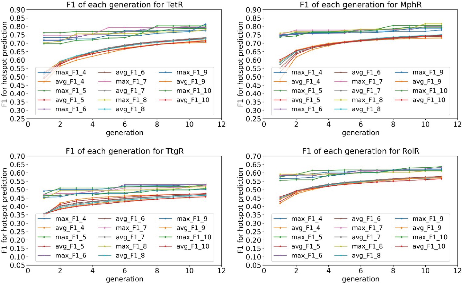
Average and best F1 scores of 4–10 feature combinations converge after 10 generations in the genetic algorithm feature selection.
The plots show the average and best F1 scores for 4–10 feature combinations as a function of generation in the genetic algorithm feature selection for the four homologous allosteric transcription factors (aTFs) as labeled by figure titles.
Figure 4—figure supplement 7
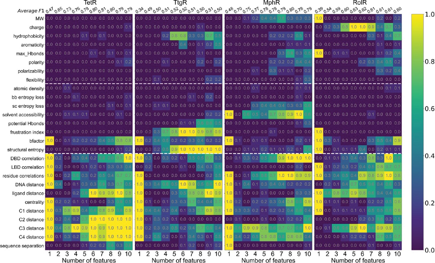
Machine learning identifies structural and molecular features that differentiate allosteric hotspots.
Frequency of appearance of the 27 features in the top ten 1–10 feature combinations ranked by F1 score for each protein (labeled on top). Row 2–28 corresponds to feature 1–27, row 1 is the average F1 score of the top ten 1–10 feature combinations. This is the same data as that of Figure 4B with all the frequencies specified in the heatmap.
Figure 4—figure supplement 8
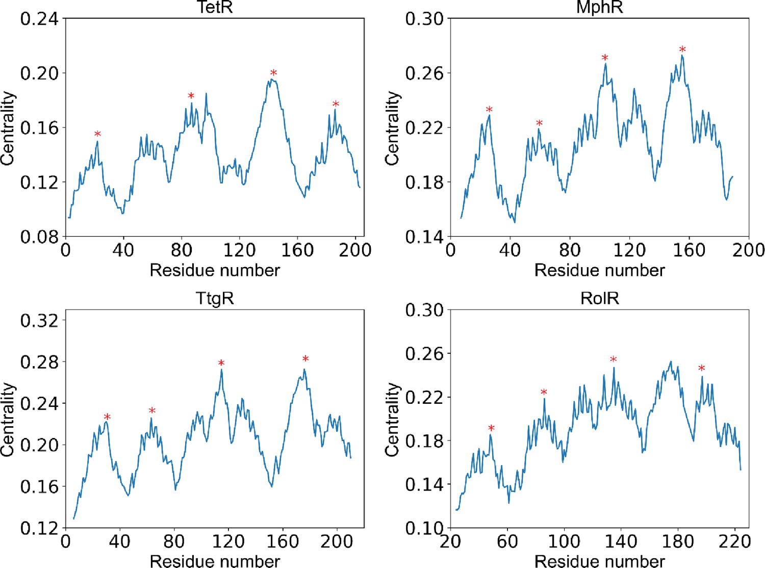
Positions of centrality peaks.
Plots of centrality against residue number of each protein (labeled by the title), with the four red stars label the positions of centrality peaks 1–4 from left to right. The centrality peaks are identified as positions of highest centrality within local sequence while maintaining distances between centrality peaks as large as possible. The centrality peaks 1–4 are located at residue 22, 83, 150, 193 for TetR; residue 26, 59, 104, 155 for MphR; residue 30, 71, 122, 186 for TtgR; and residue 48, 84, 133, 191 for RolR.
Figure 5

Cross-protein prediction – predicting allosteric hotspots in one homolog using data from other homologs.
(A) Best cross-protein predictions without (CPP, yellow) and with transfer learning (CPP_TL, green) achieved for each protein using models trained with 1–10 features and different training data. The title of each heatmap specifies the target protein being predicted. The label of each row indicates the training dataset used (a protein name means data from that one protein and homologs means data from all other three proteins besides the target protein). The first row reports the best fivefold cross-validation performance achieved using 1–10 features on the target protein, and the first column (marked ‘0’) is the performance of a random model for comparison. The row of 10%_TargetProtein indicates the best performance of neural networks (NNs) trained with only 10% data of the target protein in predicting the rest 90% data. (B) Comparison of hotspot predictions of MphR using different models (all employing features 17, 20, 21, 25, 26). Residue numbers of MphR are marked horizontally. Experimental data is the first row; ‘MphR’ shows the result of fivefold cross-validation performance of the NN on the MphR data; ‘10% MphR’ shows the performance of NN trained with 10% MphR data in predicting the rest 90%; ‘Homologs – CPP’ and ‘Homologs – CPP_TL’ shows cross-protein prediction without and with transfer learning of NN trained with data of the other three homologs in predicting MphR.
Figure 6 with 1 supplement
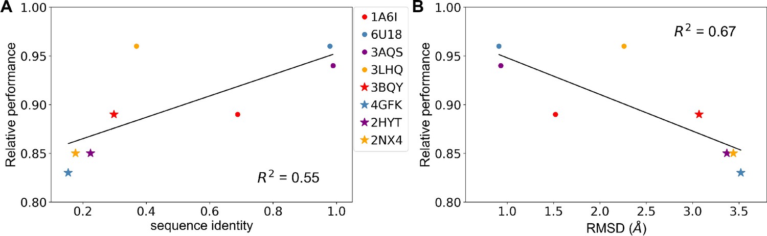
Predicting allosteric hotspots using homology models.
(A) Correlation between relative performance and the identity between the template protein and the target protein for modeling. (B) Correlation between relative performance and the root mean squared distance (RMSD) between the template protein and the target protein for modeling. R squared shows the coefficient of determination of the corresponding linear regression (red: templates for TetR; blue: templates for MphR; purple: templates for RolR; orange: templates for TtgR).
Figure 6—figure supplement 1
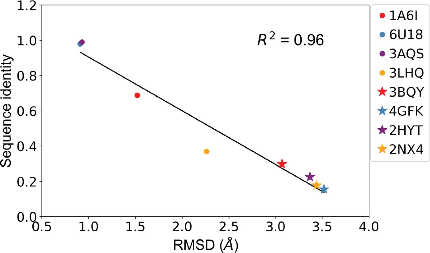
Sequence identity and root mean squared distance (RMSD) between template protein and target protein are anticorrelated.
Correlation of sequence identity and RMSD between the four allosteric transcription factors (aTFs) and their corresponding templates used in generating homology models. R squared shows the coefficient of determination of the corresponding linear regression (red: templates for TetR; blue: templates for MphR; purple: templates for RolR; orange: templates for TtgR).
Tables
Table 1
Mutation phenotype prediction performancea.
| TetR | MphR | RolR | TtgR | |
|---|---|---|---|---|
| UniRep1900 | 0.50±0.01 | 0.65±0.00 | 0.57±0.01 | 0.43±0.01 |
| feat1927 | 0.53±0.00 | 0.69±0.00 | 0.59±0.02 | 0.44±0.00 |
| random | 0.11 | 0.12 | 0.09 | 0.07 |
-
a. Performances are evaluated as the average performance of five times of fivefold cross-validation tests; Unirep1900 and feat1927 show best NN performance using only Unirep features and using Unirep features in combination with 27 physical features, respectively. Data are presented as average ± std.
Table 2
Hotspot prediction performancea.
| TetR | MphR | RolR | TtgR | |
|---|---|---|---|---|
| feat27 | 0.83±0.02 | 0.82±0.02 | 0.64±0.02 | 0.54±0.03 |
| UniRep1900 | 0.61±0.07 | 0.50±0.02 | 0.32±0.03 | 0.35±0.03 |
| random | 0.19 | 0.16 | 0.26 | 0.21 |
-
a. Feat27 represents the fitness of the best-performing feature combination emerged in feature selection with the GA-NN approach. Performances are evaluated as the average performance of five times of fivefold cross-validation tests, and presented as average ± std.
Additional files
-
Supplementary file 1
Pairwise sequence identity and similarity.
- https://cdn.elifesciences.org/articles/79932/elife-79932-supp1-v2.docx
-
Supplementary file 2
R squared correlation of deads identified at each position between replicates.
- https://cdn.elifesciences.org/articles/79932/elife-79932-supp2-v2.docx
-
Supplementary file 3
Cluster rankings.
- https://cdn.elifesciences.org/articles/79932/elife-79932-supp3-v2.docx
-
Supplementary file 4
Template information.
- https://cdn.elifesciences.org/articles/79932/elife-79932-supp4-v2.docx
-
Supplementary file 5
Cross-protein prediction of mutation phenotype.
- https://cdn.elifesciences.org/articles/79932/elife-79932-supp5-v2.zip
-
MDAR checklist
- https://cdn.elifesciences.org/articles/79932/elife-79932-mdarchecklist1-v2.pdf
Download links
A two-part list of links to download the article, or parts of the article, in various formats.
Downloads (link to download the article as PDF)
Open citations (links to open the citations from this article in various online reference manager services)
Cite this article (links to download the citations from this article in formats compatible with various reference manager tools)
Deep mutational scanning and machine learning reveal structural and molecular rules governing allosteric hotspots in homologous proteins
eLife 11:e79932.
https://doi.org/10.7554/eLife.79932


