A stochastic model of hippocampal synaptic plasticity with geometrical readout of enzyme dynamics
- Université Côte d’Azur, France
- Institut de Pharmacologie Moléculaire et Cellulaire (IPMC), CNRS, France
- Inria Center of University Côte d’Azur (Inria), France
- Neuroscience and Mental Health Research Innovation Institute, Division of Psychological Medicine and Clinical Neurosciences,School of Medicine, Cardiff University, United Kingdom
- School of Computing, Engineering, and Intelligent Systems, Magee Campus, Ulster University, United Kingdom
- School of Computer Science, Electrical and Electronic Engineering, and Engineering Mathematics, University of Bristol, United Kingdom
Figures
Figure 1
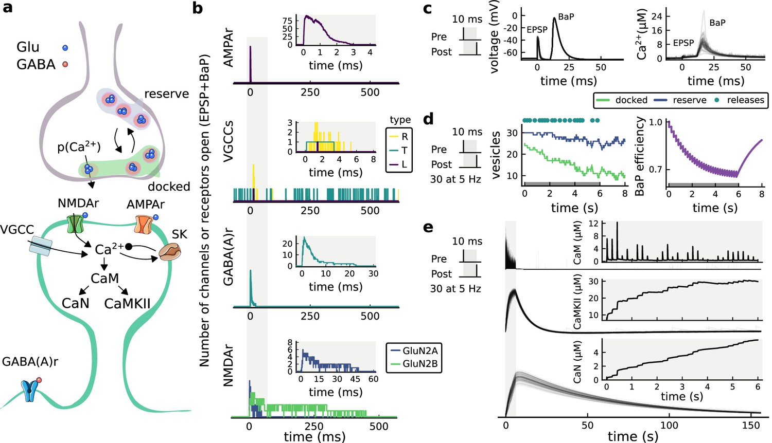
| The synapse model, its timescales and mechanisms.
(a), Model diagram with the synaptic components including pre and postsynaptic compartments and inhibitory transmission (bottom left). AMPAr, NMDAr: AMPA- and NMDA-type glutamate receptors respectively; GABA(A)r: Type A GABA receptors; VGCC: R-, T- and L-type voltage-gated Ca2+ channels; SK: SK potassium channels. (b), Stochastic dynamics of the different ligand-gated and voltage-gated ion channels in the model. Plots show the total number of open channels as a function of time. The insets show a zoomed time axis highlighting the difference in timescale of the activity among the channels. (c), Dendritic spine membrane potential (left) and calcium concentration (right) as function of time for a single causal (1Pre1Post10) stimulus (EPSP: single excitatory postsynaptic potential, ‘1Pre’; BaP: single back-propagated action potential, ‘1Post’). (d), Left: depletion of vesicle pools (reserve and docked) induced by 30 pairing repetitions delivered at 5 Hz (Sterratt et al., 2011), see Materials and methods. The same depletion rule is applied to both glutamate- and GABA-containing vesicles. Right: BaP efficiency as function of time. BaP efficiency phenomenologically captures the distance-dependent attenuation of BaP (Buchanan and Mellor, 2007; Golding et al., 2001), see Materials and methods. (e), Concentration of active enzyme for CaM, CaN, and CaMKII, as function of time triggered by 30 repetitions of 1Pre1Post10 pairing stimulations delivered at 5 Hz. The vertical grey bar is the duration of the stimuli, 6 s. The multiple traces in the graphs in panels c (right) and e reflect the run-to-run variability due to the inherent stochasticity in the model.
Figure 2
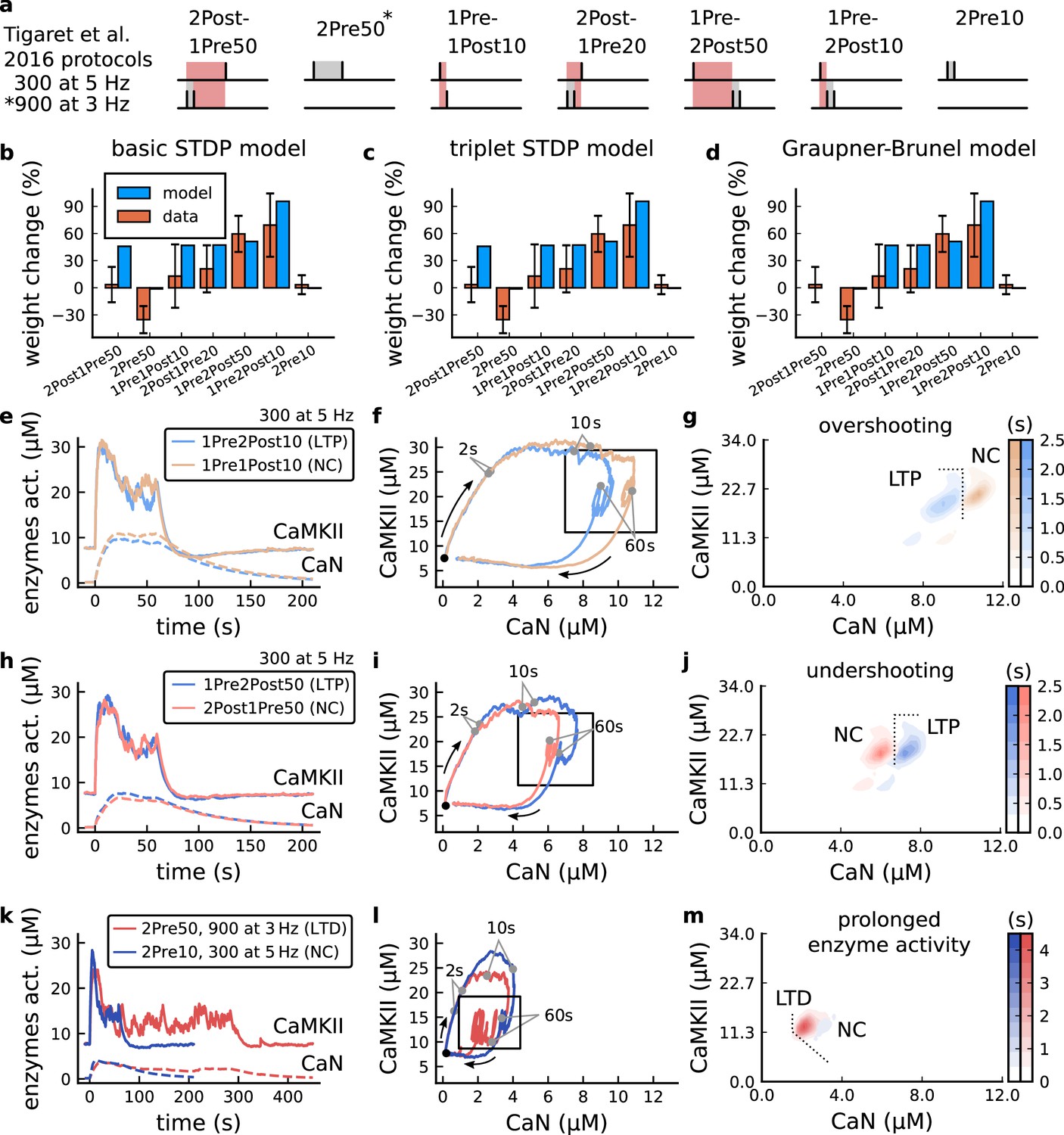
| The duration and amplitude of the joint CaN-CaMKII activity differentiates plasticity protocols.
(a), Tigaret et al., 2016 protocols, which inspired this model.(a) is adapted from Figure 2B from Tigaret et al., 2016. (b–d), Standard models for predicting plasticity fail to account for Tigaret et al., 2016 data. Mean weight change for the Tigaret’s data (red), error bars denote ±1 s.d. Plasticity protocols indicated by labels on x-axis. Blue bars show mean plasticity predicted for the same protocols by classic STDP model (Song et al., 2000) (panel b), triplet STDP model (Pfister and Gerstner, 2006) (panel c), or Graupner-Brunel calcium-based STDP (Graupner and Brunel, 2012) model (panel d). (e), Time-course of active enzyme concentration for CaMKII (solid line) and CaN (dashed line) triggered by two protocols consisting of 300 repetitions at 5 Hz of 1Pre2Post10 or 1Pre1Post10 stimulus pairings. Protocols start at time 0 s. Experimental data indicates that 1Pre2Post10 and 1Pre1Post10 produce LTP and no change (NC), respectively. (f), Trajectories of joint enzymatic activity (CaN-CaMKII) as function of time for the protocols in panel e, starting at the initial resting state (filled black circle). The arrows show the direction of the trajectory and filled grey circles indicate the time points at 2, 10, and 60 s after the beginning of the protocol. The region of the CaN-CaMKII plane enclosed in the black square is expanded in panel g. (g), Mean-time (colorbar) spent by the orbits in the CaN-CaMKII plane region expanded from panel f for each protocol (average of 100 samples). For panels g, j and m the heat maps were based on enzyme and 2Post1Pre50 (NC) depicted in the same manner as in panels (e-g). (k-m), CaN-CaMKII activities for the LTD-inducing protocol 2Pre50 (900 repetitions at 3 Hz) and the NC protocol 2Pre10 (300 repetitions at 5 Hz) depicted in the same manner as in panels e-g.
Figure 3 with 4 supplements
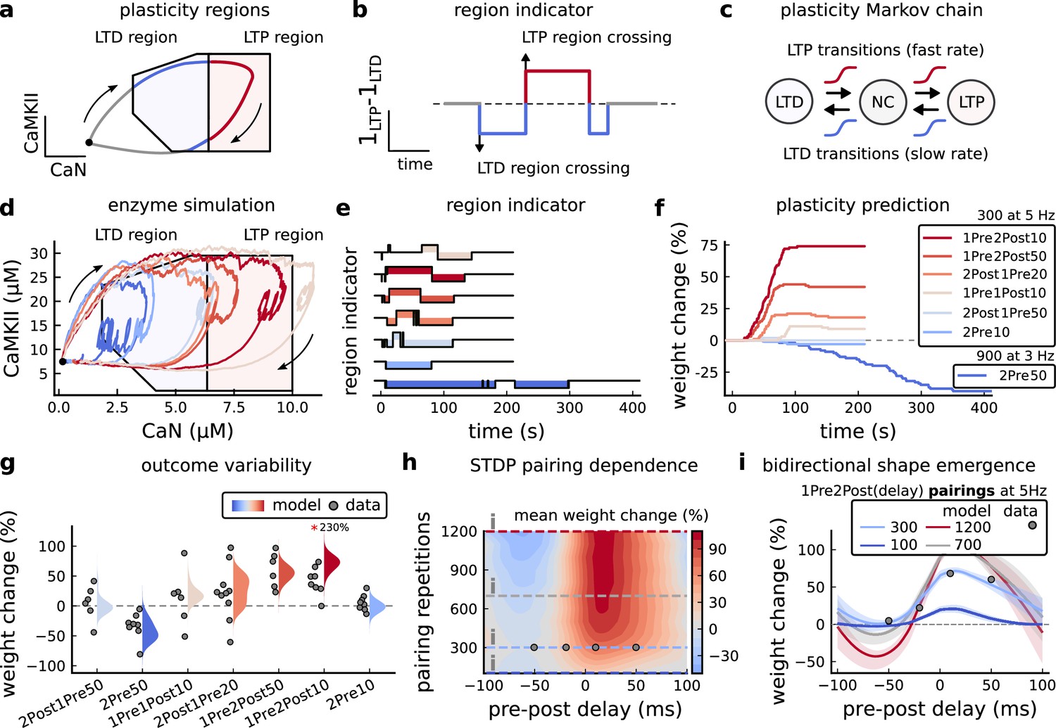
Read-out strategy to accurately model Tigaret et al., 2016 experiment.
(a) Illustration of the joint CaMKII and CaN activities crossing the plasticity regions. Arrows indicate the flow of time, starting at the filled black circle. (b) Region indicator showing when the joint CaN and CaMKII activity crosses the LTD or LTP regions in panel a. For example, the LTP indicator is such that if and 0 otherwise. Leaving the region activates a mechanism with a slow timescale that keeps track of the accumulated time inside the region. Such mechanism drives the transition rates used to predict plasticity (Materials and methods). (c), Plasticity Markov chain with three states: LTD, LTP and NC. There are only two transition rates which are functions of the plasticity region indicator (Materials and methods). The LTP transition is fast, whereas the LTD transition is slow, meaning that LTD change requires longer time inside the LTD region (panel a). The NC state starts with 100 processes. See Figure 23 for more details on the dynamics of the Plasticity Markov Chain. (d) Joint CaMKII and CaN activity for all protocols in Tigaret et al., 2016 (shown in panel f). The stimulus ends when the trajectory becomes smooth. Trajectories correspond to those in Figure 2b, e and h, at 60 s. (e) Region indicator for the protocols in panel f. The upper square bumps are caused by the protocol crossing the LTP region, the lower square bumps when the protocol crosses the LTD region (as in panel d). (f) Synaptic weight (%) as function of time for each protocol. The weight change is defined as the number (out of 100) of states in the LTP state minus the number of states in the LTD state (panel c). The trajectories correspond to the median of the simulations in panel g. (g) Synaptic weight change (%) predicted by the model compared to data (EPSC amplitudes) from Tigaret et al., 2016 (100 samples for each protocol, also for panel h and i). The data (filled grey circles) was provided by Tigaret et al., 2016 (note an 230% outlier as the red asterisk). (h) Predicted mean synaptic weight change (%) as a function of delay (ms) and number of pairing repetitions (pulses) for the protocol 1Pre2Post(delay), where delays are between –100 and 100 ms. LTD is induced by 2Post1Pre50 after at least 500 pulses. The mean weight change along the horizontal dashed line is reported in the STDP curves in panel i. (i) Synaptic weight change (%) as a function of pre-post delay. Each plot corresponds to a different pairing repetition number (color legend). The solid line shows the mean, and the ribbons are the 2nd and 4th quantiles. The filled grey circles are the data means estimated in Tigaret et al., 2016, also shown in panel g.
Figure 3—figure supplement 1
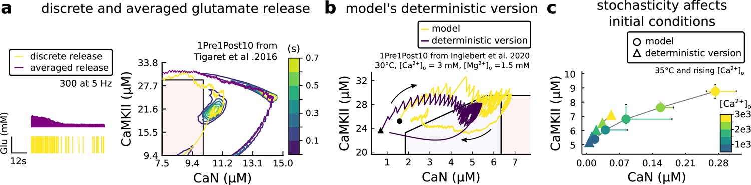
Comparison showing different roles of stochasticity in the model.
(a) Left, Glutamate concentration from a single realization of the model (yellow) and averaged Glutamate concentration (purple) from 100 repetitions of the model for 300 pulses train at 5 Hz. Right, 1Pre1Post10 from Tigaret et al., 2016 using the model (yellow) and a version of the model (purple) in which the glutamate concentration is the average one (as in Left panel). The time spent (s) is shown for the different glutamate release modes (stochastic and averaged) with an example trajectory (purple and solid yellow lines). There are no failures in averaged release; therefore, enzymes are over-activated. (b) A comparison between our model and a fully deterministic version for the 1Pre1Post10 from Inglebert et al., 2020. Note the significant mismatch, which does not allow the deterministic model to reach the LTP region that determines the plasticity outcome. This effect is mainly caused by the stochastic calcium sources, which the deterministic model fails to reproduce. The black triangle (circle) marks the initial conditions of the deterministic model. This initial condition is reached by letting the model evolve with no input. (c) The initial conditions are increasingly different when comparing the model and its fully deterministic version for rising concentrations of external calcium concentrations.
Figure 3—figure supplement 2
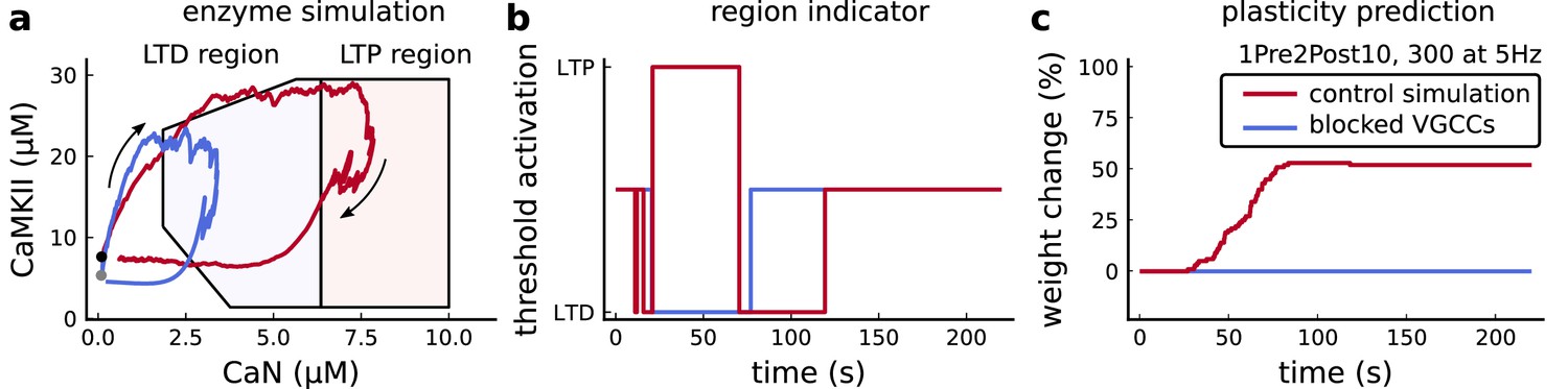
Effects of blocking VGCCs.
(a), Combined enzyme activity of the experiment 1Pre2Post10, 300 at 5 Hz described in Tigaret et al., 2016 with and without VGCCs (legend in panel c). The arrows indicate time flow, and the grey and black dots represent the initial conditions. Note the effect of VGCC blocking on the initial conditions. (b), Region indicator associated to panel a. (c) Plasticity prediction for the simulated experiment with and without VGCCs. Note that when VGCCs are blocked LTP cannot be induced, in agreement with Tigaret et al., 2016 experimental data.
Figure 3—figure supplement 3
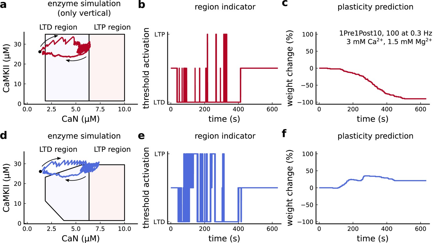
Exclusively setting vertical boundaries (no CaMKII selectivity) fails to capture the correct plasticity outcome.
(a) Combined activity of the protocol 1Pre1Post10, 100 at 0.3 Hz with experimental conditions as in Figure 6c considering the polygonal regions responding only to CaN thresholds. Note that most of the activity resides in the LTD region. The arrows indicate time flow and black dot represents the initial condition. (b) Region indicator related to panel a. (c) Plasticity prediction shows LTD, instead of LTP. (d) Same as a but considering the plasticity regions sensitivity both to CaMKII and CaN. (e) Region indicator related to panel d. (f) Plasticity prediction for panel d showing LTP agreeing with data described in Figure 6c.
Figure 3—figure supplement 4
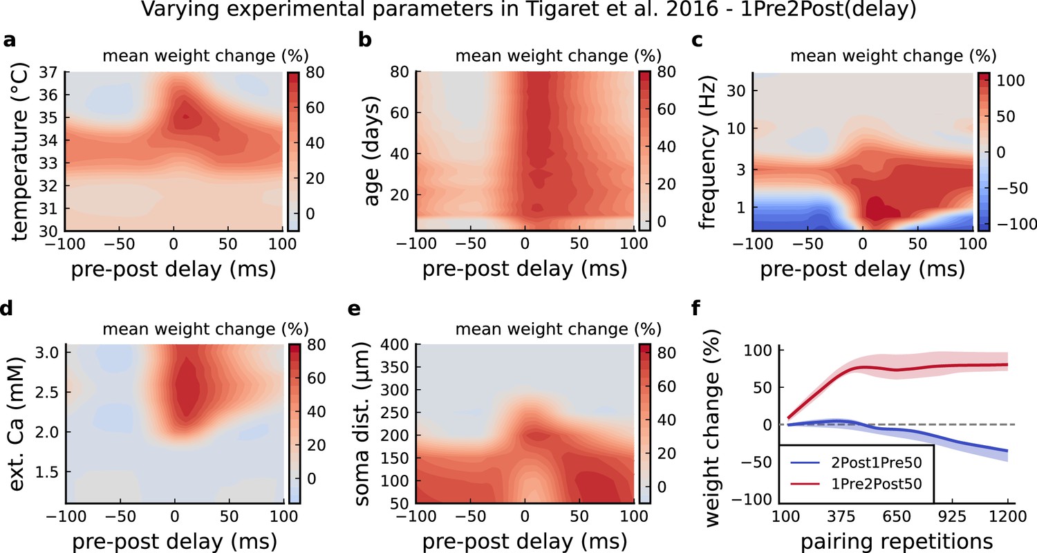
Varying Tigaret et al., 2016 experimental parameters.
(a) Mean synaptic weight change for 1Pre2Post(delay) varying the temperature. (b) Mean synaptic weight change for 1Pre2Post(delay) varying the age. (c) Mean synaptic weight change for 1Pre2Post(delay) varying the frequency. (d) Mean synaptic weight change for 1Pre2Post(delay) varying the [Ca2+]o. (e) Mean synaptic weight change for 1Pre2Post(delay) varying the distance from the soma. A similar trend in distal spines was previously found in Ebner et al., 2019. (f) Mean synaptic weight change of 1Pre2Post50 and 2Post1Pre50 when number of pulses increases or decreases. Note the similarity with Mizuno et al., 2001 in Figure 6—figure supplement 1f .
Figure 4 with 2 supplements
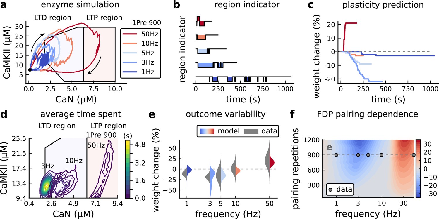
Frequency dependent plasticity (FDP), Dudek and Bear, 1992 dataset.
(a) Example traces of joint CaMKII-CaN activity for each of Dudek and Bear, 1992 protocol. (b) Region indicator showing when the joint CaMKII-CaN activity crosses the LTD or LTP regions for each protocol in panel a. (c) Synaptic weight change (%) as a function of time for each protocol, analogous to Figure 3c. Trace colours correspond to panel a. The trajectories displayed were chosen to match the medians in panel e. (d) Mean (100 samples) time spent (s) for protocols 1Pre for 900 pairing repetitions at 3, 10, and 50 Hz. (e), Comparison between data from Dudek and Bear, 1992 and our model (1Pre 900 p, 300 sampcomles per frequency, see Appendix 1—table 1). Data are represented as normal distributions with the mean and variance of the change in field EPSP slope taken from Dudek and Bear, 1992. (f), Prediction for the mean weight change (%) when varying the stimulation frequency and pulse number (24x38 × 100 data points, respectively pulse x frequency x samples). The filled grey circles show the Dudek and Bear, 1992 protocol parameters and the corresponding results are shown in panel e. In Figure 4—figure supplement 1, we provide additional graphs of frequency dependent plasticity outcomes, including predictions, when varying experimental parameters in Dudek and Bear, 1992 (external Mg, external Ca, distance from soma, temperature, Poisson spike train during development).
Figure 4—figure supplement 1
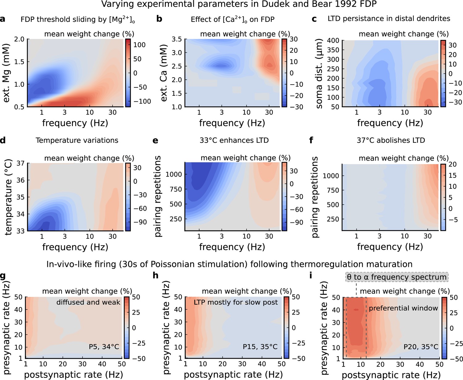
Varying experimental parameters in Dudek and Bear, 1992 and Poisson spike train during development.
(a) Mean synaptic weight change for the FDP experiment varying the [Mg2+]o. Original [Mg2+]o in Dudek and Bear, 1992 is 1.5 mM (dashed grey line). (b) Mean synaptic weight change for the FDP experiment varying the [Ca2+]o. Original [Ca2+]o in Dudek and Bear, 1992 is 2.5 mM (dashed grey line). (c) Mean synaptic weight change for the FDP experiment varying the distant from the soma. Original distance in Dudek and Bear, 1992 is 200 µm (dashed grey line). Changing the distance from the soma modifies how fast BaPs evoked by EPSP will attenuate. Note that LTD is prevalent for a spine situated far from the soma. (d) Mean synaptic weight change for the FDP experiment varying the temperature. Original temperature in Dudek and Bear, 1992 is 35°C (dashed grey line). (e) Mean synaptic weight change for the FDP experiment varying the pairing repetitions at 33°C showing how LTD is enhanced. (f) Mean synaptic weight change for the FDP experiment varying the pairing repetitions at 37°C showing how LTD is abolished. (g) Mean synaptic weight change for pre and postsynaptic Poisson spike train during 30 s for P5 and 34°C. The panel shows that there is weak and diffused LTP. (h) Mean synaptic weight change for pre and postsynaptic Poisson spike train during 30 s for P15 and 35°C. The panel shows that there is a start of LTP window forming for slow postsynaptic rates (<1 Hz). (i) Mean synaptic weight change for pre and postsynaptic Poisson spike train during 30 s for P20 and 35°C. The panel shows that a window forms around 10 Hz postsynaptic rate similar to what is shown by Graupner et al., 2016 and in Figure 7h. From these simulations, we can provide several predictions. The external Mg controls the sliding threshold (panel a). By analysing how the concentration of external calcium modifies the BCM-like curve we suggest that stimulation patterns used by Dudek and Bear are unlikely to produce LTD at more physiological calcium concentrations (1–1.5 mM). This also suggests that LTD is more likely to be driven by burst instead of slow firing (panel b). LTP and LTD generation are both affected by the distance of the synapses from the soma (panel c). A similar analysis was done by Ebner et al., 2019 describing a similar prediction. We show that LTD is more prone to variations of amplitude by temperature than LTP (panels 1- d,e,f). We predict that stimuli of Poissonian spike trains differently shape the plasticity outcome depending on the animal’s age (panels 1 g,h,i).
Figure 4—figure supplement 2
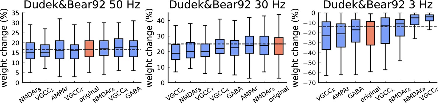
The figure shows the weight change (%) for Dudek and Bear, 1992 protocols (50 Hz, 30 Hz, and 3 Hz, related to Figure 4 of the main manuscript).
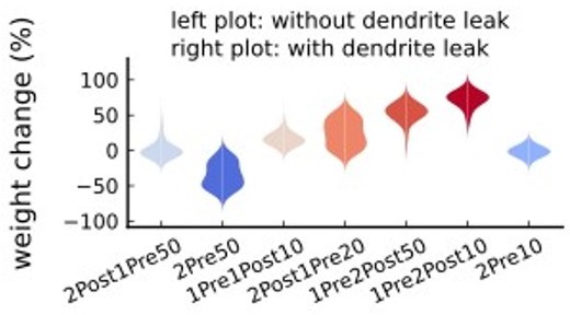
The blue bars represent a single model component changed from stochastic to deterministic (100 simulations per condition). The red bars represent the original model. The horizontal lines in all panels indicate the expected experimental outcome. The model components are ordered in the x-axis from the lowest to the highest weight change. The deterministic equations were determined from the reactions rates described in the Materials and methods and generated by the Julia package Catalyst.jl. The deterministic substitution for each element has different effects. This is attributed to stochasticity having different roles for each protocol. It is clear in Dudek and Bear, 1992 - 3 Hz that any of the stochastic components of our model cannot be substituted without causing alterations in the model outcomes. Regardless of the number of channels/receptors in our synapse model, the deterministic substitution cannot guarantee the same results.
Figure 5 with 1 supplement
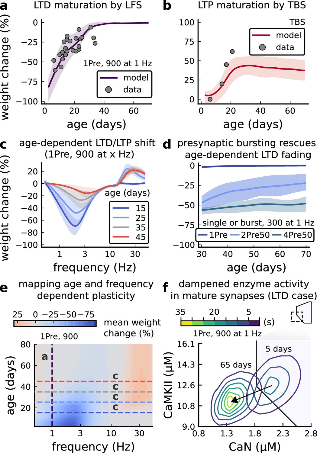
Age-dependent plasticity, Dudek and Bear, 1993 dataset.
(a), Synaptic weight change for 1Pre, 900 at 1 Dudek and Bear, 1993. The solid line is the mean and the ribbons are the 2nd and 4th quantiles predicted by our model (same for panel b, c and f). (b), Synaptic weight change for theta burst stimulation (TBS - 4Pre at 100 Hz repeated 10 times at 5 Hz given in 6 epochs at 0.1 Hz, see Appendix 1—table 1). (c), Synaptic weight change as a function of frequency for different ages. BCM-like curves showing that, during adulthood, the same LTD protocol becomes less efficient. It also shows that high-frequencies are inefficient at inducing LTP before P15. (d), Synaptic weight change as a function of age. Proposed protocol using presynaptic bursts to recover LTD at ≥ P35 with less pulses, 300 instead of the original 900 from Dudek and Bear, 1993. This effect is more pronounced for young rats. Figure 5—figure supplement 1 shows a 900 pulses comparison. (e), Mean synaptic strength change (%) as a function of frequency and age for 1Pre 900 pulses (32x38 × 100, respectively, for frequency, age and samples). The protocols in Dudek and Bear, 1993 (panel a) are marked with the yellow vertical line. The horizontal lines represent the experimental conditions of panel c. Note the P35 was used for Dudek and Bear, 1992 experiment in Figure 4f. (f), Mean time spent for the 1Pre 1 Hz 900 pulses protocol showing how the trajectories are left-shifted as rat age increases. In Figure 5—figure supplement 1, we provide additional simulations to analyse the synaptic plasticity outcomes, including predictions, of duplets, triplets and quadruplets for FDP, perturbing developmental-mechanisms for Dudek and Bear, 1993, and age-related changes in STDP experiments (Inglebert et al., 2020; Tigaret et al., 2016; Meredith et al., 2003).
Figure 5—figure supplement 1
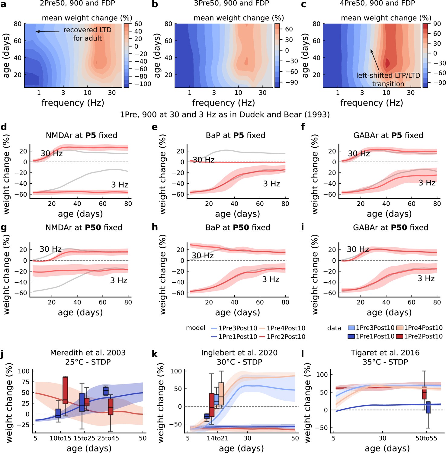
Duplets, triplets, and quadruplets for FDP, perturbing developmental-mechanisms for Dudek and Bear, 1993, and age-related changes in STDP experiments (Inglebert et al., 2020; Tigaret et al., 2016; Meredith et al., 2003).
(a) Mean synaptic weight change (%) for the duplet-FDP (2Pre50) experiment varying age. The panel shows showing that not only LTD is enhanced but also LTP. (b) Mean synaptic weight change (%) for the triplet-FDP (3Pre50) experiment varying age. The panel shows that LTD magnitude is enhanced for adult rats and the LTD-LTP transition is shifted leftward. (c) Mean synaptic weight change (%) for the quadruplet-FDP (4Pre50) experiment varying age. The panel shows a further leftward shift on the LTD-LTP transition (compared to 3Pre50). (d) Mean synaptic weight change (%) for the 1 Pre 900 at 30 and 3 Hz with Dudek and Bear, 1993. Fixing NMDAr at P5 (more GluN2B than GluN2A) causes an increase of LTD and a slight increase of LTP for adult rats compared to baseline (grey solid line). (e) Same experiment as panel d but fixing BaP maturation at P5 (higher BaP attenuation). LTP is abolished, but LTD is not affected. This is because AP induced by the EPSP attenuate too fast for 30 Hz and are thus not able to produce enough depolarization to activate NMDArs. (f) Same experiment as in panel d but fixing GABAr maturation at P5 (excitatory GABAr) which only slighlty enhances LTD (3 Hz) for adult rats. (g) Same experiment as panel d but fixing NMDAr at P50 (more GluN2A than GluN2B). LTD appears with decreased magnitude for young rats compared to baseline (grey solid line). (h) Same experiment as panel d but fixing BaP maturation at P50 (less BaP attenuation). LTP is enhanced for young rats because the BaP pairing with the slow closing GluN2B produces more calcium influx. (i) Same experiment as panel d but fixing GABAr maturation at P50 (inhibitory GABAr) which does not affect the FDP experiment. (j) Mean synaptic weight change (%) for Meredith et al., 2003 single versus burst-STDP experiment for different ages. The data from Meredith (boxplots) were pooled by the age as shown in the x-axis. The solid line represents the mean, and the shaded ribbon the 2nd and 4th quantiles simulated by the model (same for panels a-f). (k) Mean synaptic weight change (%) for Inglebert et al., 2020 STDP experiment in which the number of postsynaptic spikes increases. The x-axis marker from 14 to 21 indicates that only this interval was published without further specification. We use our model to estimate age related changes to Inglebert et al., 2020 protocols. Note that the model does not cover the 1Pre2Post10 properly (model predicts only outcomes near the first data quantile). Notice that single and burst STDP leads to LTD, meanwhile Meredith et al., 2003 lead to LTP or NC. (l), Mean synaptic weight change (%) for Tigaret et al., 2016 STDP experiment which compares single versus burst STDP. The x-axis marker from 50 to 55 indicates that only a interval was published without further specification. We use our model to estimate age related changes to Tigaret et al., 2016 protocols. It is noticeable that each STDP experiment has a different development. We highlight some predictions that could occur in non-physiological conditons. If BaP maturation doesn’t occur, that is, BaP is always inefficient, then LTP cannot be induced by high frequencies. Also, if NMDAr are principally composed of the GluN2B subunit, meaning that the receptor does not go through the age-dependent maturation process, then LTD would remain pronounced at higher ages.
Figure 6 with 2 supplements
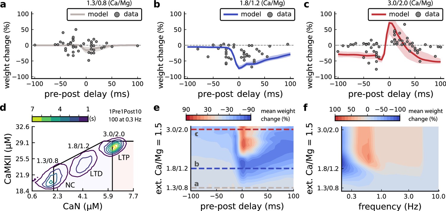
Effects of extracellular calcium and magnesium concentrations on plasticity.
(a), Synaptic weight (%) for a STDP rule with [Ca2+]o=1.3 mM (fixed ratio, Ca/Mg = 1.5). According to the data extracted from Inglebert et al., 2020, the number of pairing repetitions for causal/positive (anti-causal/negative) delays is 100 (150), both delivered at 0.3 Hz. The solid line is the mean, and the ribbons are the 2nd and 4th quantiles predicted by our model (all panels use 100 samples). (b), Same as a, but for [Ca2+]o = 1.8 mM (Ca/Mg ratio = 1.5). (c), Same as a, but for [Ca2+]o = 3 mM (Ca/Mg ratio = 1.5). (d), Mean time spent for causal pairing, 1Pre1Post10, at different Ca/Mg concentration ratios. The contour plots are associated with the panels a, b and c. e, Predicted effects of extracellular Ca/Mg on STDP outcome. Synaptic weight change (%) for causal (1Pre1Post10, 100 at 0.3 Hz) and anticausal (1Post1Pre10, 150 at 0.3 Hz) pairings varying extracellular Ca from 1.0 to 3 mM (Ca/Mg ratio = 1.5). The dashed lines represent the experiments in the panel a, b and c. We used 21x22 × 100 data points, respectively calcium x delay x samples. (f), Predicted effects of varying frequency and extracellular Ca/Mg for an STDP protocol. Contour plot showing the mean synaptic weight (%) for a single causal pairing protocol (1Pre1Post10, 100 samples) varying frequency from 0.1 to 10 Hz and [Ca2+]o from 1.0 to 3 mM (Ca/Mg ratio = 1.5). We used 21 x 18 × 100 data points, respectively calcium x frequency x samples.
Figure 6—figure supplement 1
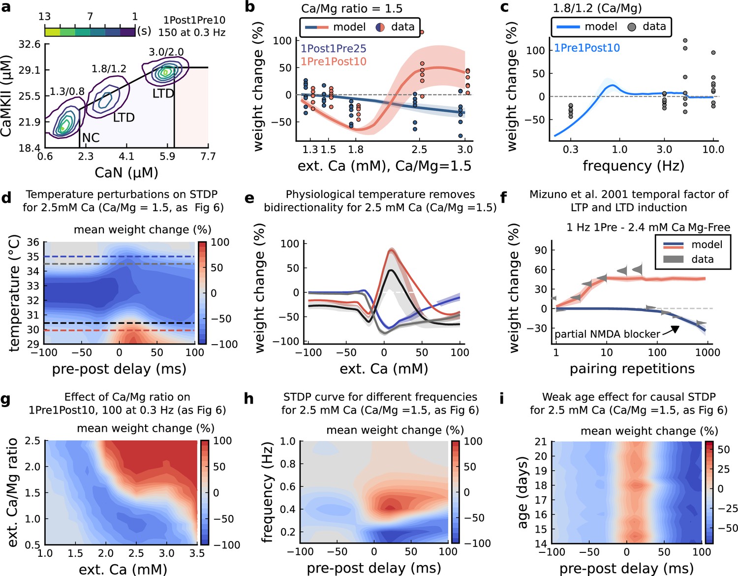
[Ca2+]o and [Mg2+]o related modifications for Inglebert et al., 2020 experiment.
(a), Mean time spent for anticausal pairing, 1Post1Pre10, at different Ca/Mg concentrations. The contour plots are associated with the Figure 6a–c. (b), STDP and extracellular Ca/Mg. Synaptic weight change (%) for causal (1Pre1Post10, 100 at 0.3 Hz) and anticausal (1Post1Pre10, 150 at 0.3 Hz) pairings varying [Ca2+]o from 1.0 to 3 mM (Ca/Mg ratio = 1.5). (c), Varying frequency and extracellular Ca/Mg for the causal pairing 1Pre1Post10, 100 at 0.3 Hz. Synaptic weight change (%) for a single causal pairing protocol varying frequency from 0.1 to 10 Hz. [Ca2+]o was fixed at 1.8 mM (Ca/Mg ratio = 1.5). (d), Mean synaptic weight change (%) for Inglebert et al., 2020 STDP experiment showing how temperature qualitatively modifies plasticity. The dashed lines are ploted in panel b. (e), Mean synaptic weight change (%) showing the effects of 0.5°C change in panel d. Black and grey solid lines represent the same color dashed lines in panel d (30 and 30.5°C). The bidirectional curves, black and grey lines in panel d (dashed) and panel e (solid), becoming full-LTD when temperature increases to 34.5 and 35°C, respectively yellow and purple lines in panel d (dashed) and panel e (solid). Further increase abolishes plasticity. f, Mean synaptic weight change (%) for Mizuno et al., 2001 experiment in Mg-Free ([Mg2+]o = 10-3 mM for best fit) showing the different time requirements to induce LTP and LTD. For LTD, to simulate the NMDAr antagonist D-AP5 which causes a NMDAr partial blocking we reduced the NMDAr conductance by 97%. Note the similarity with Figure 3—figure supplement 4f. (g), Mean synaptic weight change (%) of Inglebert et al., 2020 STDP experiment changing [Ca2+]o and Ca/Mg ratio. (h), Mean synaptic weight change (%) of Inglebert et al., 2020 STDP experiment changing pre-post delay time and frequency. Note the similarity with Figure 3—figure supplement 4c. (i), Mean synaptic weight change (%) of Inglebert et al., 2020 STDP experiment changing pre-post delay time and age. Age has a weak effect on this experiment done at [Ca2+]o = 2.5 mM.
Figure 6—figure supplement 2
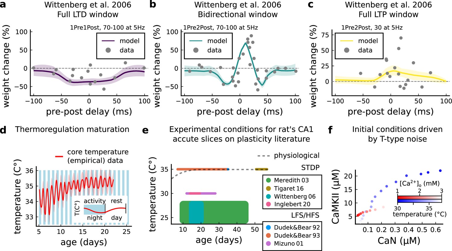
Temperature and age effects.
(a), Mean synaptic weight change (%) for Wittenberg and Wang, 2006 STDP experiment for 1Pre1Post10, 70–100 at 5 Hz (see Appendix 1—table 1) showing a full LTD window. Our model also reproduces the data showing that when temperature is increased to LTD is abolished (data not shown). (b) Mean synaptic weight change (%) for Wittenberg and Wang, 2006 STDP experiment for 1Pre2Post10, 70–100 at 5 Hz (see Appendix 1—table 1) showing a bidirectional window. (c) Mean synaptic weight change (%) for Wittenberg and Wang, 2006 STDP experiment for 1Pre2Post10, 20–30 at 5 Hz (see Appendix 1—table 1) showing a bidirectional window. We noticed that for Wittenberg and Wang, 2006 experiment, done in room temperature, the temperature sensitivity was higher than for other experiments. (d) Core temperature varying with age representing the thermoregulation maturation. This function (not shown) was fitted using rat (Wood et al., 2016) and mouse data (McCauley et al., 2020) added by 1°C to compensate species differences (Wood et al., 2016). The blue and white bars represent the circadian rhythm as shown in McCauley et al., 2020. However, the ‘rest rhythm’ for young rats (P5-14) may vary. (e), Dotted grey line represents the averaged physiological temperature at different ages in the rat (estimated from mean value of panel d). For the papers the we fitted by the model, we depict the range of temperature and age used. Note that only few experiments were performed at near physiological conditions. (f) Initial conditions for CaN-CaMKII resting concentration for different [Ca2+]o and temperature values. When [Ca2+]o is changed, temperature is fixed at 35°C, while when temperature is changed, [Ca2+]o is fixed at 2 mM.
Figure 7
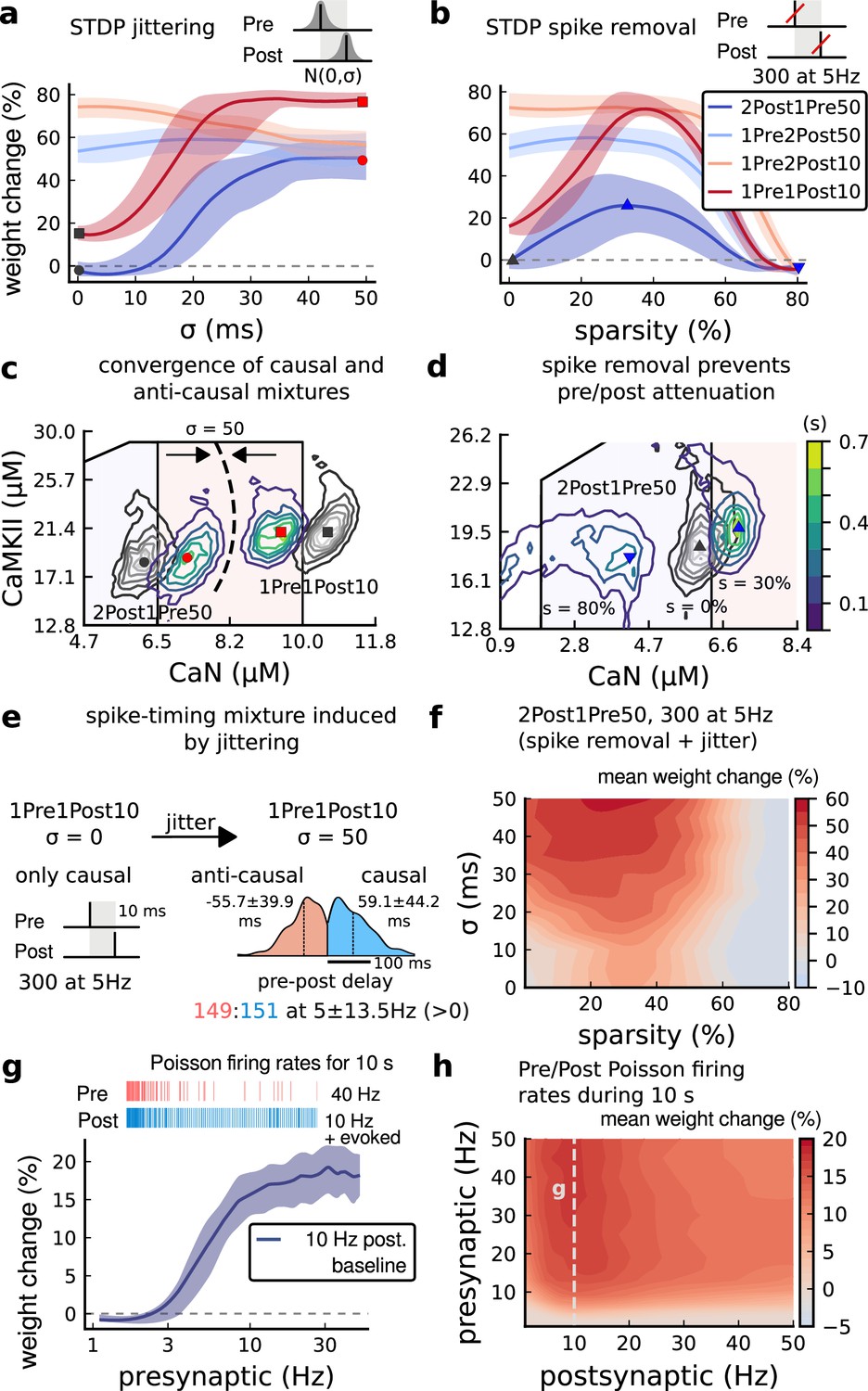
Jitter and spike dropping effects on STDP and Poisson spike trains.
(a) Mean weight (%) for the jittered STDP protocols (protocol color legend shown in b). The solid line is the mean, and the ribbons are the 2nd and 4th quantiles predicted by our model using 100 samples (same for panels a, b and g). (b) Mean weight (%) for the same (Tigaret et al., 2016) protocols used in panel a subjected to random spike removal (sparsity %). (c) Effect of jitttering on Mean time (s) spent by joint enzymes trajectories in LTP/LTD regions. Contour plot shows 2Post1Pre50 and 1Pre1Post10 (300 at 5 Hz) without (grey contour plot) and with jittering (coloured contour plot). The circles and squares correspond to the marks in panel a. (d) Effect of sparsity on Mean time (s) spent by joint enzymes trajectories in LTP/LTD regions. Contour plot in grey showing 0% sparsity for 2Post1Pre50 300 at 5 Hz (see Figure 2j). The contour plots show the protocol with spike removal sparsities at 0% (NC), 30% (LTP), and 80% (NC). The triangles correspond to the same marks in panel a. (e) Distribution of the 50 ms jittering applied to the causal protocol 1Pre1Post10, 300 at 5 Hz in which nearly half of the pairs turned into anticausal. The mean frequency is 5 ±13.5 Hz making it to have a similar firing structure and position in the LTP region. The similar occurs for 2Post1Pre50 (panel c). (f) Mean weight change (%) combining both jittering (panel a) and sparsity (panel b) for 2Post1Pre50, 300 at 5 Hz. (g) Mean weight change (%) of pre and postsynaptic Poisson spike train delivered simultaneously for 10 s. The plot shows the plasticity outcome for different presynaptic firing rate (1000/frequency) for a fixed postsynaptic baseline at 10 Hz. The upper raster plot depicts the released vesicles at 40 Hz and the postsynaptic baseline at 10 Hz (including the AP evoked by EPSP). (h) Mean weight change (%) varying the rate of pre and postsynaptic Poisson spike train delivered simultaneously for 10 s. The heat map data along the vertical white dashed line is depicted in panel g.
Figure 8
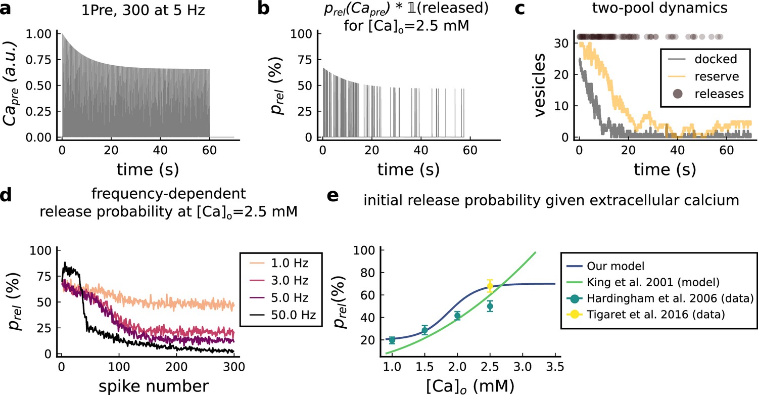
Presynaptic release model validation.
(a) Presynaptic calcium in response to the protocol 1Pre, 300 pulses at 5 Hz displaying adaptation. (b) Release probability for the same protocol as panel A but subjected to the docked vesicles availability. (c) Number of vesicles in the docked and reserve pools under depletion caused by the stimulation from panel a. (d) Plot of the mean (300 samples) release probability (%) for different frequencies for the protocol 1Pre 300 pulses at [Ca2+]o = 2.5 mM. (e) Release probability (%) for a single presynaptic spike as a function of [Ca2+]o. Note that King et al., 2001 model was multiplied by the experimentally measured release probability at [Ca2+]o = 2 mM since their model has this calcium concentration as the baseline.
Figure 9
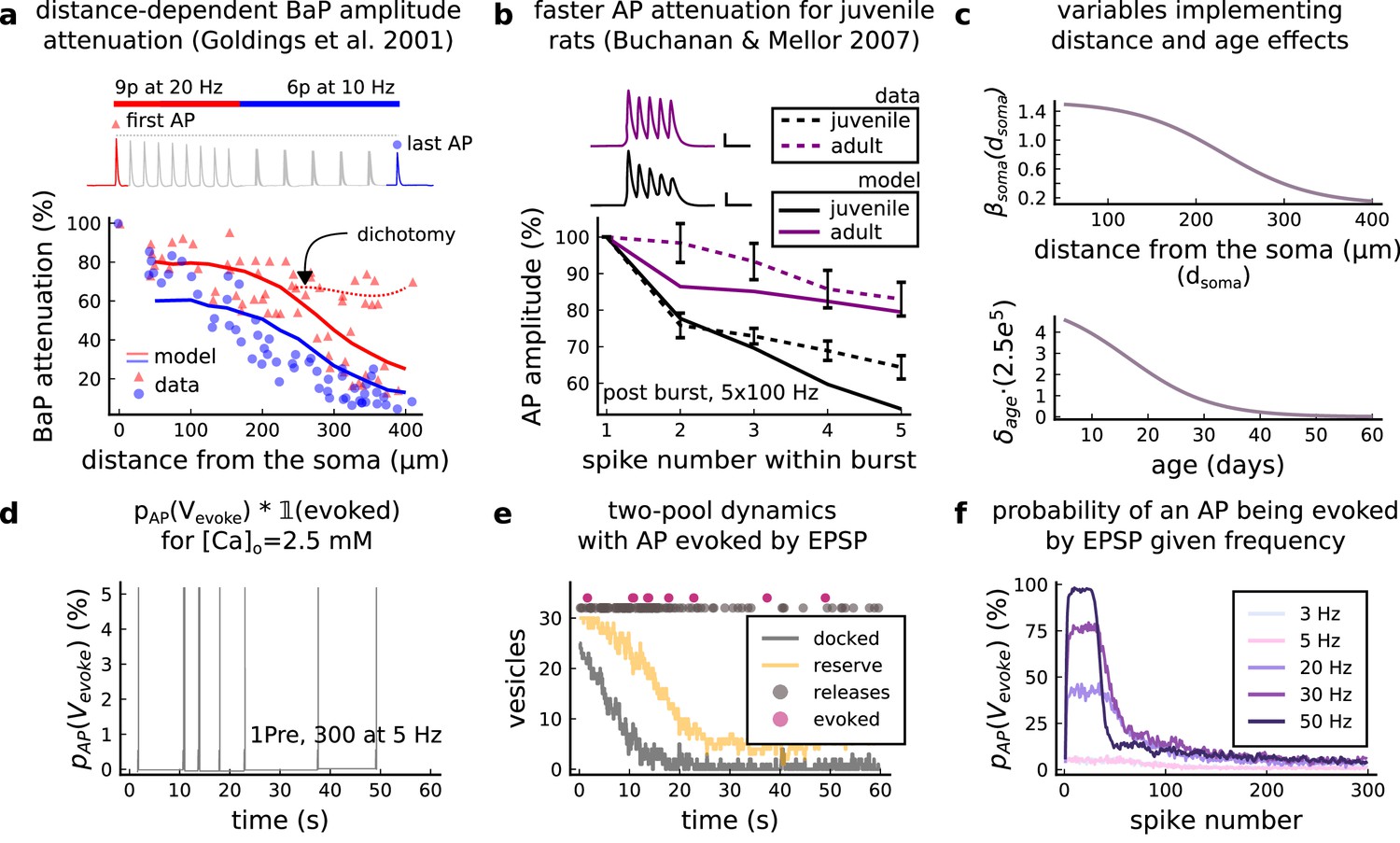
AP Evoked by EPSP.
(a) Model and data comparison for the distance-dependent BaP amplitude attenuation measured in the dendrite and varying the distance from the soma. The stimulation in panel a is set to reproduce the same stimulation as Golding et al., 2001. Golding described two classes of neurons: those that are strongly attenuated and those that are weakly attenuated (dichotomy mark represented by the dashed line). However, in this work we consider only strongly attenuated neurons. (b) Attenuation of somatic action potential from Buchanan and Mellor, 2007 and model in response to five postsynaptic spikes delivered at 100 Hz. The value showed for the model is the spine voltage with distance from the soma set to zero (scale 25 ms, 20 mV). (c) Top panel shows the used in Equation 6 to modify the axial conductance between the soma and dendrite. Bottom panel shows the age-dependent changes in the step of the resource-use equation (Equation 7) that accelerates the BaP attenuation and decreases the sodium currents in Equation 5. (d) Probability of evoking an AP multiplied by the successfully evoked AP, , for the protocol 1Pre, 300 at 5 Hz (2.5 mM Ca). (e) Two-pool dynamics with the same stimulation from panel D showing the vesicle release, the reserve and docked pools, and the evoked AP. (f) Probability of evoking an AP for the protocol 1Pre 300 pulses at different frequencies (3 and 5 Hz have the same probability).
Figure 10
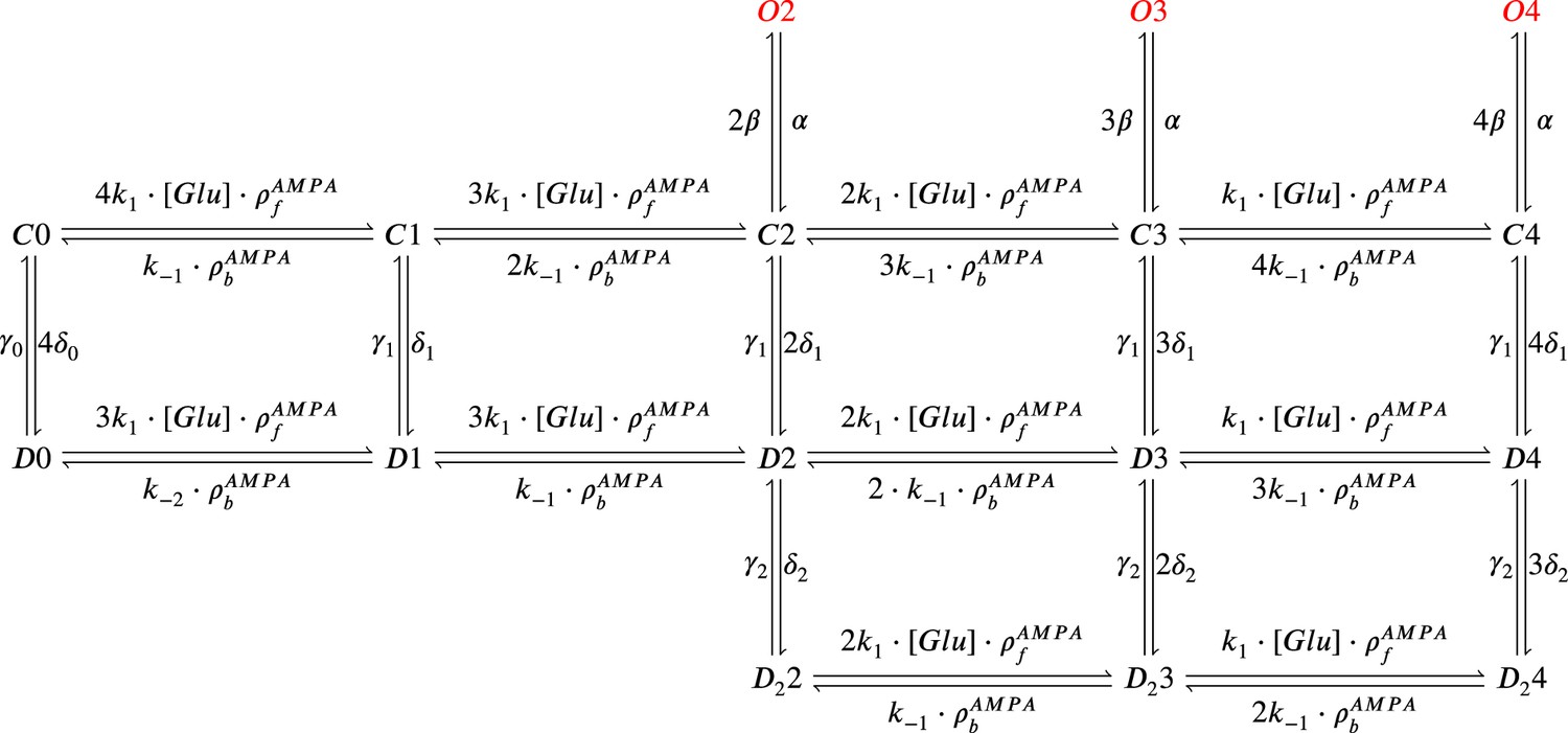
AMPAr Markov chain with three sub-conductance states and two desensitisation levels.
It includes parameters , (binding and unbinding of glutamate) which depend on temperature. Open states are , , and ; closed states are , , , , and ; desensitisation states are , , , , and ; deep desensitisation states are , , and .
Figure 11
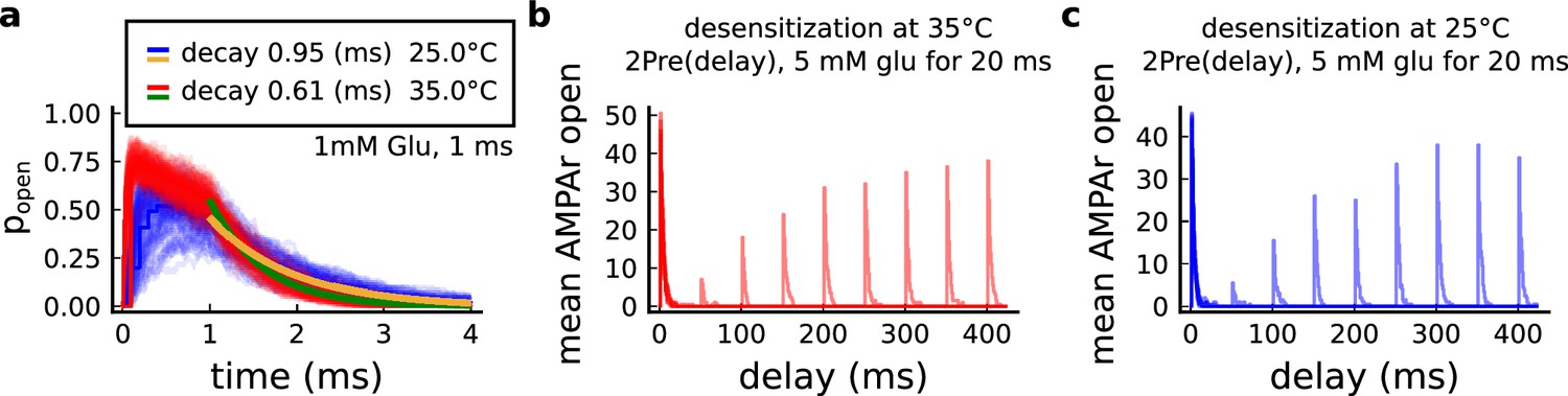
Effect of temperature on AMPArs.
(a) Probability of AMPAr opening () and the decay time at different temperatures, in response to 1 mM glutamate applied for 1 ms (standard pulse). Postlethwaite et al., 2007 data (our model) suggests that AMPAr decay time at 35°C is () and at 25°C is (). This shows a closer match towards more physiological temperatures. (b) Desensitisation profile of AMPAr at 35°C showing how many AMPAr are open in response to repeated glutamate saturating pulses (5 mM Glu for 20 ms) separated by an interval (x-axis). (c) Same as in panel b but for 25°C.
Figure 12
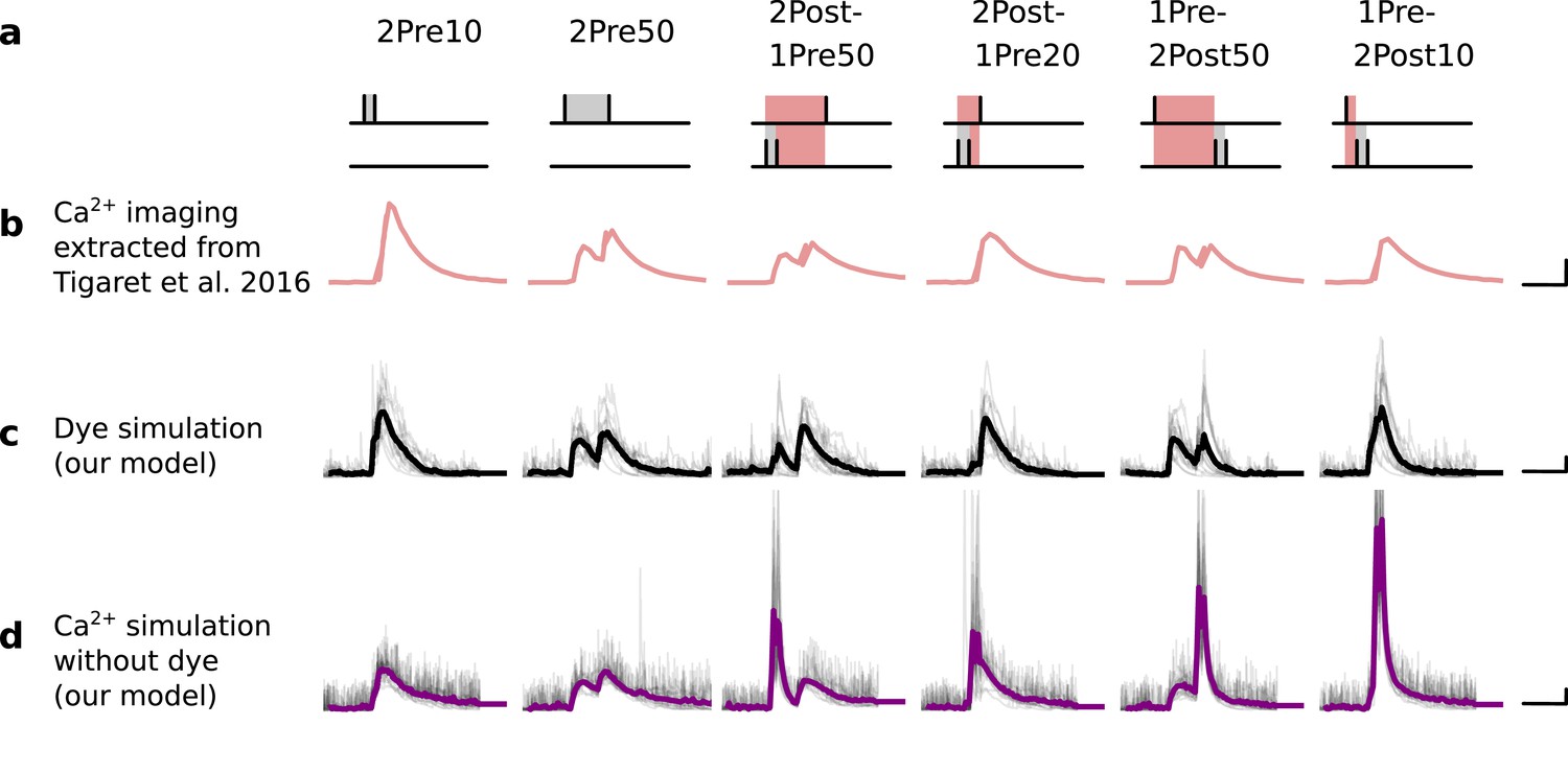
Differences between dye measurements and simulated calcium.
(a), Pre and postsynaptic stimuli as used in Tigaret et al., 2016. (b), Calcium imaging curves (fluorescence ΔF/A) elicited using the respective stimulation protocols above with Fluo5 200 μM (extracted from Tigaret et al., 2016). Scale 100 ms, 0.05 ΔF/A. (c), Dye simulation using the model. The dye is implemented by increasing temperature to mimic laser effect on channel kinetics and decreases the interaction between NMDAr and voltage elicited by BaP. Temperature effects over NMDAr are shown in Korinek et al., 2010. Also, the effects of temperature on calcium-sensitive probes shown in Oliveira et al., 2012 (baseline only, likely related to T-type channels). Other examples of laser heating of neuronal tissue are given in Deng et al., 2014. Such a dye curve fitting was obtained by increasing temperature by 10°C to mimic laser-induced heating (Wells et al., 2007; Deng et al., 2014). We achieved a better fit by decreasing the amplitude of the BaP that reaches the dendrite. Additionally, for fitting purposes, we assumed that a temperature increase lead to a decrease in BaP amplitude. Scale 0.6 µM dye, 100 ms. (d), Calcium simulation without dye. Scale 0.85 µM Ca2+, 100 ms.
Figure 13
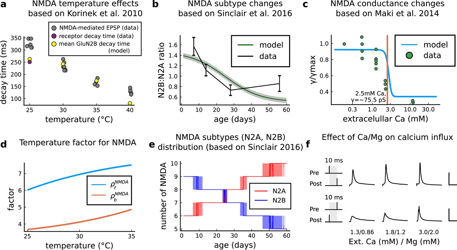
NMDAr changes caused by age, temperature and extracellular and magnesium concentrations in the aCSF.
(a) Decay time of the NMDAr-mediated EPSP recorded from neocortical layer II/III pyramidal neurons (grey) (Korinek et al., 2010) compared to the decay time from the GluN2B channel estimated by our model (yellow) and data from Iacobussi’s single receptor recording (purple) (Iacobucci and Popescu, 2018). (b), Comparison of our model of the GluN2B:GluN2A ratio and the GluN2B:GluN2A ratio from the mouse CA1 excitatory neurons. (c), Comparison of our model of NMDAr conductance change as a function of extracellular calcium, against data (Maki and Popescu, 2014). (d), Forward and backwards temperature factors implemented to approximate NMDAr subtypes decay times at room temperature (Iacobucci and Popescu, 2018) and temperature changes observed in Korinek et al., 2010. (e), NMDAr subtype number in our model as a function of animal age. We added noise to have a smoother transition between different ages. (f), Calcium concentration changes for causal and anticausal protocols in response to different aCSF calcium and magnesium compositions with fixed Ca/Mg ratio (1.5). Scale bars 50 ms and 5 μM.
Figure 14
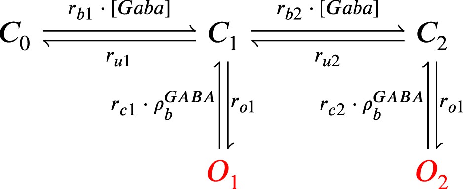
GABAr Markov chain model.
Closed states (, and ) open in response to GABAr and can go either close again or open ( and ).
Figure 15
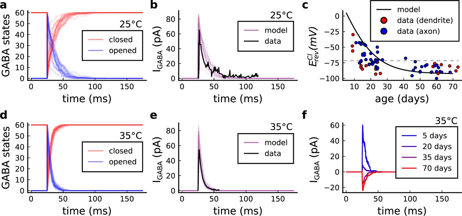
GABA(A)r current, kinetics and chloride reversal potential.
(a) States of GABA(A)r Markov chain at 25°C in response to a presynaptic stimulation. Opened = , closed = . (b) Model and data comparison (Otis and Mody, 1992) for GABA(A)r current at 25°C. Even though data were recorded from P70 at 25°C and P15 at 35°C, we normalize the amplitude to invert the polarity and compare the decay time. This is done since the noise around P15 can either make GABAr excitatory or inhibitory as shown by data in panel c. (c) Chloride reversal potential () fitted to Rinetti-Vargas et al., 2017 data. Note that we used both profiles from axon and dendrite age-depended changes since exclusive dendrite data is scarce. (d) States of simulated GABA(A)r Markov chain at 35°C in response to a presynaptic stimulation. (e) Model and data comparison (Otis and Mody, 1992) for GABA(A)r current at 25°C (same normalization as in panel b). (f) Change in the polarization of GABA(A)r currents given the age driven by the .
Figure 16
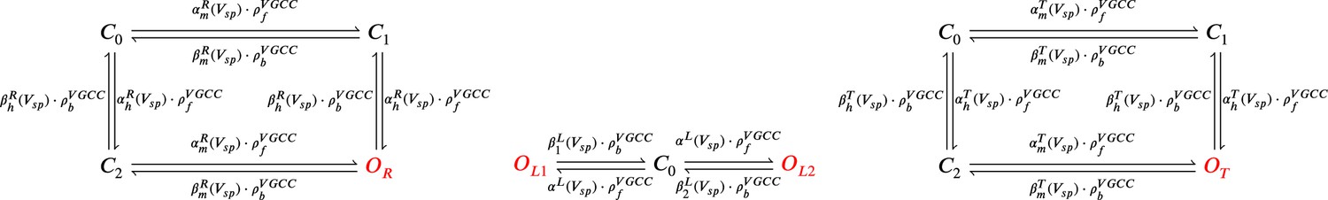
From left to right, R-, L-, and T-type VGCCs Markov chain adapted from Magee and Johnston, 1995.
The R- (left scheme) and T- type (right scheme) have a single open state (red colour), respectively, and . The L-type VGCC (middle) has two open states, and .
Figure 17
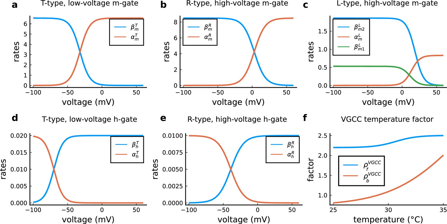
VGCC rates and temperature factors.
(a), Activation () and deactivation rates () for the T-type m-gate. (b), Activation () and deactivation rates () for the R-type m-gate. (c), Activation () and both deactivation rates ( and ) for the L-type VGCC. (d), Activation () and deactivation rates () for the T-type h-gate. (e), Activation () and deactivation rates () for the R-type h-gate. (f), Temperature factor applied to all the rates, forward change () for the rates and backward change () for the rates.
Figure 18
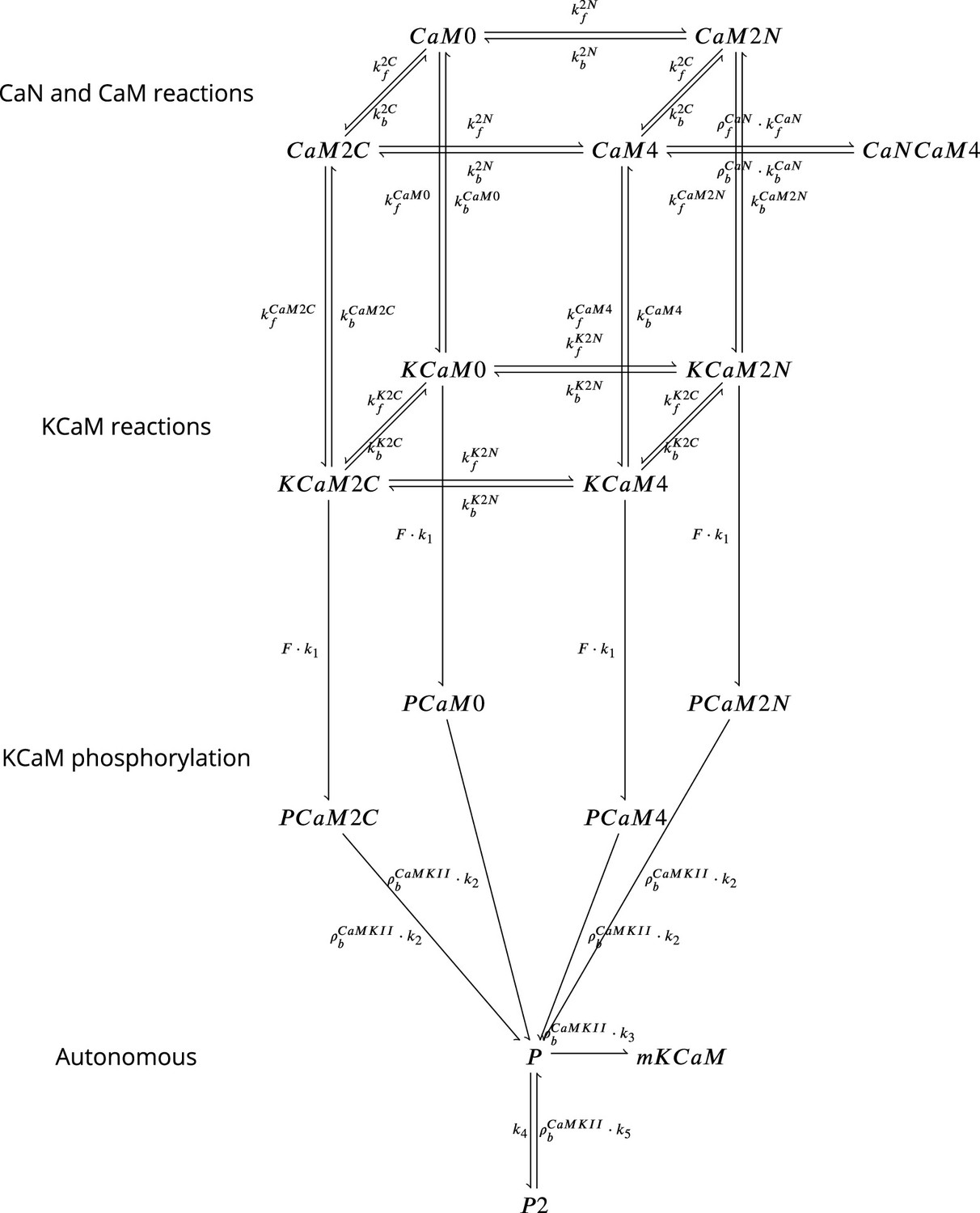
Coarse-grained model of CaM, CaMKII, and CaN adapted from Chang et al., 2019 and Pepke et al., 2010.
Figure 18 is adapted from Figure 5 from Pepke et al., 2010. Reaction from the CaM-Ca reactions (first layer) are attributed to 2Ca release and binding from different CaM saturation states CaM2C (2Ca bound to terminal C), CaM2N (2Ca bound to terminal N), CaM0 (no calcium bound), CaM4(Ca bound to both C and N terminal). Note that CaN is allowed to bind only to fully saturated CaM. Activated CaN is represented by the state CaNCaM4. Reactions between the first (CaM-Ca reactions) and the second layer (KCaM-Ca reactions) represent the binding of free/monomeric CaMKII (mKCaM) (Pepke et al., 2010) to different saturation levels of CaM. Reactions within the layer KCaM-Ca represent the binding of calcium to Calmodulin bound to CaMKII (KCaM0, KCaM2C, KCaM2N, KCaM4). Transition of layer KCaM-Ca reactions to layer KCaM-phosphorylation represents CaMKII bound to CaM that became phosphorylated (PCaM states) (Pepke et al., 2010; Chang et al., 2017; Chang et al., 2019). PCaM can become self-phosphorylated (Autonomous layer with P and P2) and release CaM. Once the KCaM deactivates from autonomous states, it returns to free monomeric CaMKII (mKCaM). The CaMKII activity in this work represent the states (KCaM +PCaM + P + P2). See Chang et al., 2019 for further explanation on this system. CaNCaM4 represents the CaN activity. For graphical reasons, we could not show the complete list of reactions as given in Table 12.
Figure 19
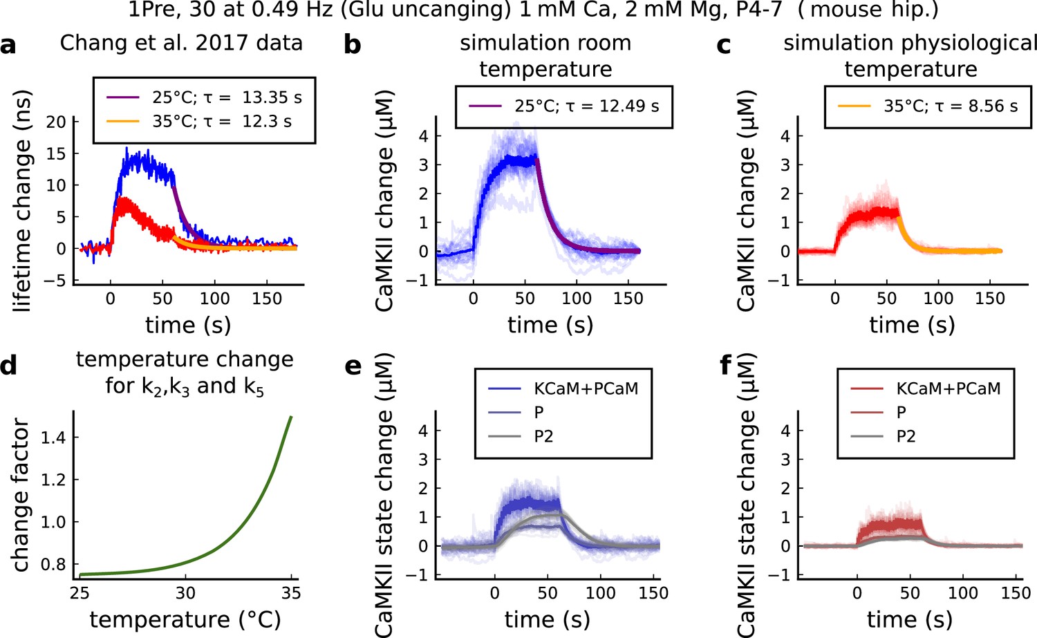
CaMKII temperature changes in the model caused by 1Pre, 30 at 0.49 Hz with glutamate uncaging (no failures allowed), 1 mM Ca, 2 mM Mg, P4-7 organotypic slices from mouse hippocampus.
(a) CaMKII fluorescent probe lifetime change measured by Chang et al., 2017 for 25°C (blue) and 35°C (red). The decay time () was estimated by fitting the decay after the stimulation (30 pulses at 0.49 Hz) using a single exponential decay, .(b) Simulation of the CaMKII concentration change (with respect to the baseline) at 25°C in response to same protocol applied in the panel a. The simulations on the panels b, c, e, f show the mean of 20 samples. (c) Same as in panel b but for 35°C. (d) Estimated temperature change factor for the dissociation rates , , and in the Markov chain in Figure 18. (e) Change in the concentration of the CaMKII states (25°C) which are summed to compose CaMKII change in the panel b. (f) Same as in panel e for 35°C with reference to the panel c.
Figure 20
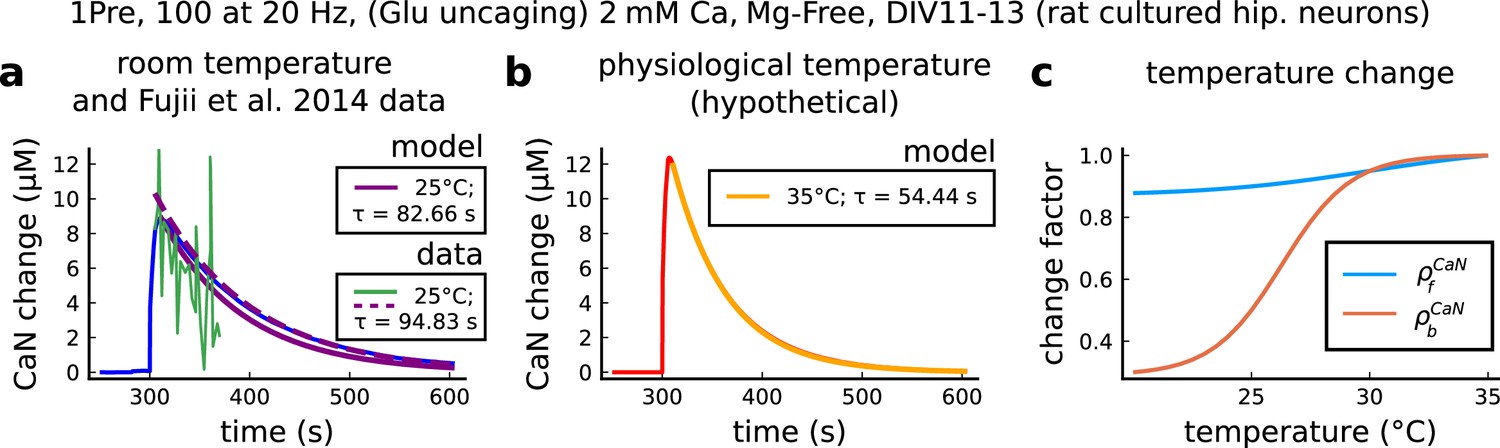
CaN temperature changes in our model caused by 1Pre, 100 at 20 Hz with glutamate uncaging (no failures allowed), 2 mM Ca, Mg-free, 11–13 days in vitro.
(a), Simulated CaN change (blue solid line) in response to the same stimuli of the CaN measurement from Fujii et al., 2013 RY-CaN fluorescent probe (green solid line). The decay time () estimated from data () is 94.83 s (dashed purple line) and 82.66 s for our model (solid purple line). (b), Simulated CaN change for physiological temperature with decay time of 54.44 s. (c), Temperature change, and , applied to CaN association and dissociation rates.
Figure 21
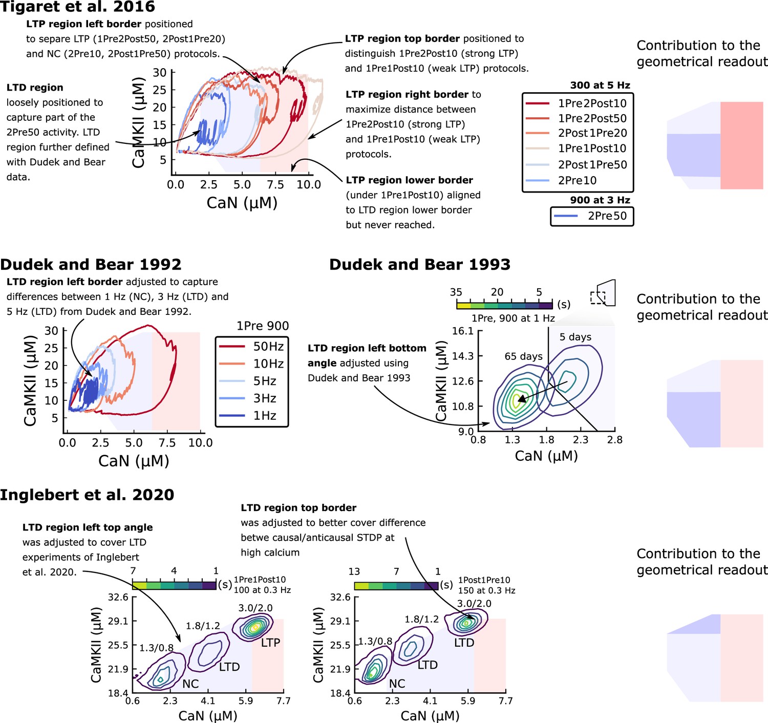
Positioning the plasticity regions.
The figure shows how Tigaret et al., 2016, Dudek and Bear, 1992, Dudek and Bear, 1993 and Inglebert et al., 2020 contributes to define the plasticity regions. In summary, Tigaret et al., 2016 data was used to define the LTP region, and Dudek and Bear, 1992, Dudek and Bear, 1993, Inglebert et al., 2020 data were used to define the LTD region.
Figure 22

Plasticity Markov Chain.
Figure 23
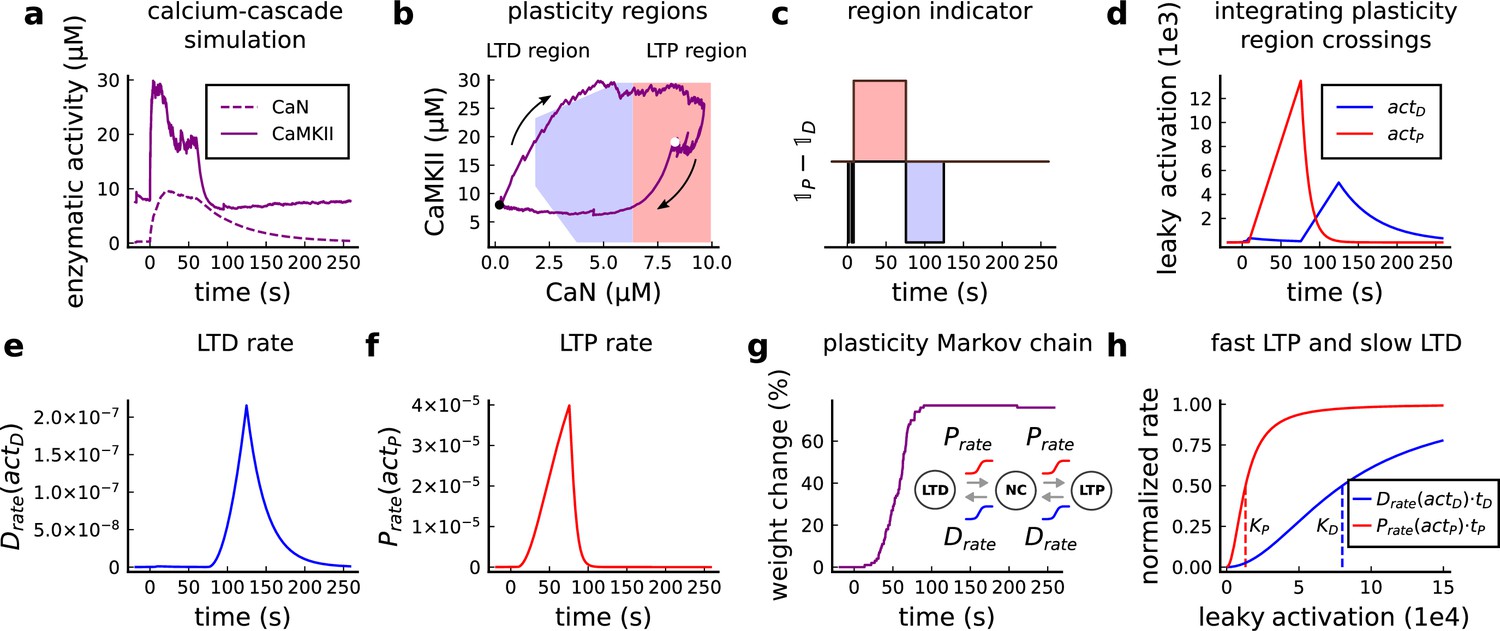
Plasticity readout for the protocol 1Pre2Post10, 300 at 5 Hz, from Tigaret et al., 2016.
(a) CaMKII and CaN activity in response to protocol 1Pre2Post10. (b) Enzymatic joint activity in the 2D plane showing LTP and LTD’s plasticity regions. The black point marks the beginning of the stimulation, and the white point shows the end of the stimulation after 60 s. (c) Region indicator illustrating how the joint activity crosses the LTP and the LTD regions. (d) The leaky activation functions are used as input to the LTP and LTD rates, respectively. The activation function has a constant rise when the joint-activity is inside the region, and exponential decay when it is out. (e) The LTD rate in response to the leaky activation function, , in panel d. Note that this rate profile occurs after the stimulation is finished (60 s). The joint-activity is returning to the resting concentration in panel A. (f) The LTP rate in response to the leaky activation function, , in panel D. (g) Outcome of the plasticity Markov chain in response to the LTD and LTP rates. The EPSP change (%) is estimated by the difference between the number of processes in the states LTP and LTD, . (h) Normalized LTP and LTD rates (multiplied to their respective time constant, , ) sigmoids. The dashed line represents the half-activation curve for the LTP and LTD rates. Note in panel d that the leaky activation function reaches the half-activation .
Author response image 1
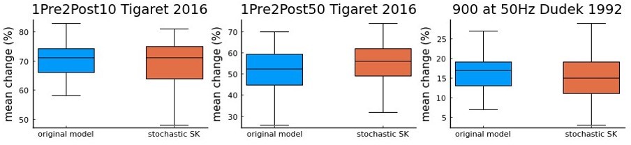
a comparison using Tigaret et al.
2016 1Pre2Post10 and 1Pre2Post50 protocols, and 900 at 50 Hz protocol from Dudek and Bear 1992 (100 repetitions) between the model with the deterministic SK channel (original model – blue), and the modified model including the stochastic SK channel (stochastic SK – red). Deterministic vs stochastic SK channel does not significantly modify the model’s behaviour.
Author response image 2
Author response image 3
Tables
Table 1
Stochastic transitions used in the presynaptic vesicle pool dynamics.
Note that the rates depend on the number of vesicles in each pool (Pyle et al., 2000).
| Transition | Rate | Initial Condition |
|---|---|---|
Table 2
Parameter values for the presynaptic model.
Our model does not implement a larger pool of ∼ 180 vesicles (CA3-CA1 hippocampus) sometimes named ‘reserve pool’ (Südhof, 2000) or ‘resting pool’ (Alabi and Tsien, 2012). Furthermore, what we term the ‘reserve pool’ in our model is sometimes called the ‘recycling pool’ in other studies, for example Rizzoli and Betz, 2005; Alabi and Tsien, 2012.
| Name | Value | Reference |
|---|---|---|
| Vesicle release model (stochastic part) | ||
| Initial number of vesicles at D | 5–20 (Rizzoli and Betz, 2005; Alabi and Tsien, 2012) | |
| Initial number of vesicles at R | 17–20 vesicles (Alabi and Tsien, 2012) | |
| Time constant R→ D (D recycling) | 1 s (Rizzoli and Betz, 2005) | |
| time constant D → R (R mixing) | 20 s (when depleted) to 5 min (hypertonic shock) (Rizzoli and Betz, 2005; Pyle et al., 2000) | |
| Time constant 1→ R (R recycling) | 20–30 s (Rizzoli and Betz, 2005) | |
| Release probability half-activation curve | see Equation 1 | |
| Release probability sigmoid slope | fixed for all [Ca2+]o | |
| Vesicle release model (deterministic part) | ||
| attenuation recovery | 50-500 ms with dye (Maravall et al., 2000) therefore < 50 to 500 ms without dye | |
| Deterministic jump attenuation recovery | ∼20 s (Rizzoli and Betz, 2005) | |
| Deterministic jump attenuation fraction | Forsythe et al., 1998 | |
Table 3
Parameters for the neuron electrical properties.
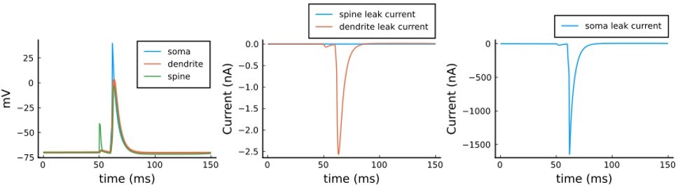
* The membrane leak conductance in the spine is small since the spine membrane resistance is so high that is considered infinite () (Koch and Zador, 1993). The current thus mostly leaks axially through the neck cytoplasm. The dendrite leak conductance is also small in order to control the distance-dependent attenuation by the axial resistance term in Equation 4 and Equation 5. The table provides the parameters associated with these equations which were adjusted (see comparison with Reference value) to fit the dynamics seen in Golding et al., 2001 and Buchanan and Mellor, 2007 experiments as in Figure 9a and b.
| Name | Value | Reference |
|---|---|---|
| Passive cable | ||
| Leak reversal potential | (Spigelman et al., 1996) | |
| Membrane leak conductance per area (for spine and passive dendrite) | * see table legend (Koch and Zador, 1993) | |
| Membrane leak conductance per area (only soma) | (Fernandez and White, 2010) | |
| Membrane capacitance per area | (Hines and Carnevale, 1997) | |
| Axial resistivity of cytoplasm | (Golding et al., 2001) | |
| Dendrite | ||
| Dendrite diameter | same as Yi et al., 2017 | |
| Dendrite length | apical dendrites, 1200–1600 μm López Mendoza et al., 2018 | |
| Dendrite surface area | ||
| Dendrite volume | ||
| Dendritic membrane capacitance | ||
| Dendrite leak conductance | ||
| Dendrite axial conductance | ||
| Soma | ||
| Soma diameter | 21 μm (Stuart et al., 2016) page 3 | |
| Soma area (sphere) | ; (Zhuravleva et al., 1997) | |
| Soma membrane capacitance | ||
| Soma leaking conductance | (Fernandez and White, 2010) | |
| Dendritic spine | ||
| Spine head volume | Bartol et al., 2015 | |
| Spine head surface | ||
| Spine membrane capacitance | ||
| Spine head leak conductance | ||
| Dendritic spine neck | ||
| Spine neck diameter | 0.05–0.6 μm Harris et al., 1992 | |
| Neck length | (Adrian et al., 2017) | |
| Neck cross-sectional area | ||
| Neck resistance | (Popovic et al., 2015) | |
Table 4
The Na +and K+conductances intentionally do not match the reference because models with passive dendrite need higher current input to initiate action potentials (Levine and Woody, 1978).
Therefore, we set it to achieve the desired amplitude on the dendrite and the dendritic spine according to the predictions of Golding et al., 2001 and Kwon et al., 2017.
| Name | Value | Reference |
|---|---|---|
| Soma parameters for Na +and K+ channel | ||
| Sodium conductance | generic value, see legend commentary | |
| Potassium conductance | generic value, see legend commentary | |
| Reversal potential sodium | Migliore et al., 1999 | |
| Reversal potential potassium | Migliore et al., 1999 | |
| BaP attenuation parameters | ||
| Attenuation step factor (age) | see Equation 7 and Figure 9b and c bottom Buchanan and Mellor, 2007; Golding et al., 2001 | |
| Attenuation step factor | adjusted to fit Buchanan and Mellor, 2007; Golding et al., 2001 | |
| Auxiliary attenuation step factor | adjusted to fit Buchanan and Mellor, 2007; Golding et al., 2001 | |
| Recovery time for the attenuation factor | adjusted to fit Buchanan and Mellor, 2007; Golding et al., 2001 | |
| Recovery time for the age attenuation factor | adjusted to fit Buchanan and Mellor, 2007; Golding et al., 2001 | |
| AP evoked by EPSP | ||
| Decay time for | Hines and Carnevale, 1997 | |
| Delay AP evoked by EPSP | Fricker and Miles, 2000 | |
Table 5
Parameter values for the AMPAr Markov chain and glutamate release affecting NMDAr, AMPAr.
Properties of GABA release are the same as those for glutamate.
| Name | Value | Reference |
|---|---|---|
| Glutamate parameters | ||
| Duration of glutamate in the cleft | Spruston et al., 1995 | |
| Concentration of glutamate in the cleft | Spruston et al., 1995 | |
| Glutamate variability (gamma distribution ) | Liu et al., 1999 | |
| Glutamate signal | for AMPAr, NMDAr and copied to GABA neurotransmitter | |
| AMPAr parameters | ||
| Number of AMPArs | =120 | Bartol et al., 2015 |
| Reversal potential | Bartol et al., 2015 | |
| Subconductance O2 | (Coombs et al., 2017) | |
| Subconductance O3 | (Coombs et al., 2017) | |
| Subconductance O4 | (Coombs et al., 2017) | |
| glu binding | Robert and Howe, 2003 | |
| glu unbinding 1 | Robert and Howe, 2003 | |
| glu unbinding 2 | Robert and Howe, 2003 | |
| Closing | Robert and Howe, 2003 | |
| Opening | Robert and Howe, 2003 | |
| Desensitisation 1 | Robert and Howe, 2003 | |
| Desensitisation 2 | Robert and Howe, 2003 | |
| Desensitisation 3 | Robert and Howe, 2003 | |
| Re-desensitisation 1 | Robert and Howe, 2003 | |
| Re-desensitisation 2 | Robert and Howe, 2003 | |
| Re-desensitisation 3 | Robert and Howe, 2003 | |
Table 6
Postsynaptic calcium dynamics parameters.
Note that the buffer concentration, calcium diffusion coefficient, calcium diffusion time constant and calcium permeability were considered free parameters to adjust the calcium dynamics.
| Name | Value | Reference |
|---|---|---|
| Buffer and dye | ||
| Association buffer constant | Bartol et al., 2015 | |
| Dissociation buffer constant | Bartol et al., 2015 | |
| Generic buffer concentration | (Bartol et al., 2015) | |
| Calcium dynamics | ||
| Calcium baseline concentration | (Maravall et al., 2000) | |
| Calcium decay time | 0.05–0.5 s with dye (Maravall et al., 2000) therefore < 0.05–0.5 s undyed (unbuffered) | |
| Calcium diffusion coefficient | (Bartol et al., 2015; Holcman et al., 2005) | |
| Calcium diffusion time constant | (Holcman et al., 2005) | |
| GHK equation | ||
| Temperature | converted to Kelvin in the Equation 14 given the protocol | |
| Faraday constant | Hille, 1978 | |
| Gas constant | Hille, 1978 | |
| Calcium permeability | adjusted to produce 3μM Calcium in response to a Glu release supplementary file from Chang et al., 2017 | |
| Calcium ion valence | Hille, 1978 | |
Table 7
NMDAr parameters.
The existing model of NMDAr (GluN2A) was adapted to obtain the NMDAr (GluN2B) model. The decay time of NMDAr (GluN2B) was fitted to match decay time in Iacobucci and Popescu, 2018 and the temperature dependence uses the EPSP decay time from Korinek et al., 2010.
Table 8
GABAr parameters.
The GABAr number and conductance were modified to fit GABAr currents as in Figure 15b and e.
| Name | Value | Reference |
|---|---|---|
| GABA(A) receptor | ||
| Number of GABAr | 30 Edwards et al., 1990 | |
| Chloride reversal potential | see age-dependent equation | fitted from Rinetti-Vargas et al., 2017 |
| GABAr conductance | 0.027 (Macdonald et al., 1989) | |
| Binding | Busch and Sakmann, 1990 | |
| Unbinding | Busch and Sakmann, 1990 | |
| Binding | Busch and Sakmann, 1990 | |
| Unbinding | Busch and Sakmann, 1990 | |
| Opening rate | Busch and Sakmann, 1990 | |
| Opening rate | Busch and Sakmann, 1990 | |
| Closing rate | temperature changes to fit Otis and Mody, 1992; Busch and Sakmann, 1990 | |
| Closing rate | temperature changes to fit Otis and Mody, 1992; Busch and Sakmann, 1990 | |
Table 9
VGCC parameters.
The number of VGCC was set to 3 to reproduce the calcium dynamics measured with a dye as in Figure 12 (Tigaret et al., 2016).
| Name | Value | Reference |
|---|---|---|
| VGCC | ||
| VGCC T-type conductance | same as Magee and Johnston, 1995 | |
| VGCC R-type conductance | same as Magee and Johnston, 1995 | |
| VGCC L-type conductance | same as Magee and Johnston, 1995 | |
| number of VGCCs | 3 for each subtype | 1–20 Higley and Sabatini, 2012 |
Table 10
SK channel parameters.
| Name | Value | Reference |
|---|---|---|
| SK channel | ||
| Number of SK channels | Lin et al., 2008 | |
| SK conductance | Maylie et al., 2004 | |
| SK reversal potential | Griffith et al., 2016 | |
| SK half-activation | Griffith et al., 2016 | |
| SK half-activation slope | 4 Griffith et al., 2016 | |
| SK time constant | Griffith et al., 2016 | |
Table 11
Concentration of each enzyme.
| Name | Value | Reference |
|---|---|---|
| Enzyme concentrations | ||
| Free CaM concentration (spine) | µM | Kakiuchi et al., 1982 |
| Free KCaM concentration (spine) | µM | Feng et al., 2011; Lee et al., 2009 |
| Free CaN spine concentration (spine) | µM | >10 μM (estimation from Kuno et al., 1992) |
Table 12
Parameters for the coarse-grained model published in Pepke et al., 2010 and adapted by Chang et al., 2019 and this work.
Pepke et al., 2010 rate adaptation for the coarse-grained model . Refer to Figure 18 for definition of variables.
| REACTIONS | Value | Reference |
|---|---|---|
| Coarse-grained model, CaM-Ca reactions | ||
| CaM0+2 Ca⇒ CaM2C CaM2N+2 Ca⇒ CaM4 | Pepke et al., 2010 | |
| CaM0+2 Ca⇒ CaM2N CaM2C+2 Ca⇒ CaM4 | Pepke et al., 2010 | |
| CaM2C⇒ CaM0+2 Ca CaM4⇒ CaM2N+2 Ca | Pepke et al., 2010 | |
| CaM2N⇒ CaM0+2 Ca CaM4⇒ CaM2C+2 Ca | Pepke et al., 2010 | |
| 1.2 to 9.6 μM-1s-1 (Pepke et al., 2010) | ||
| 5 to 35 μM-1s-1 (Pepke et al., 2010) | ||
| 25 to 260 μM-1s-1 (Pepke et al., 2010) | ||
| 50 to 300 μM-1s-1 (Pepke et al., 2010) | ||
| 10 to 70 s-1 (Pepke et al., 2010) | ||
| 8.5 to 10 s-1 (Pepke et al., 2010) | ||
| 1 . 103 to 4 . 103 s-1 (Pepke et al., 2010) | ||
| 0.5 . 103 to > 1.103 s-1 (Pepke et al., 2010) | ||
| Coarse-grained model, KCaM-Ca reactions | ||
| KCaM0+2 Ca⇒ KCaM2C KCaM2N+2 Ca⇒ KCaM4 | Pepke et al., 2010 | |
| KCaM0+2 Ca⇒ KCaM2N KCaM2C+2 Ca⇒ KCaM4 | Pepke et al., 2010 | |
| KCaM2C⇒ KCaM0+2 Ca KCaM4⇒ KCaM2N+2 Ca | Pepke et al., 2010 | |
| KCaM2N⇒ KCaM0+2 Ca KCaM4⇒ KCaM2C+2 Ca | Pepke et al., 2010 | |
| Pepke et al., 2010 | ||
| Pepke et al., 2010 | ||
| Pepke et al., 2010 | ||
| Pepke et al., 2010 | ||
| Pepke et al., 2010 | ||
| 0.49 to 4.9 s-1 (Pepke et al., 2010) | ||
| Pepke et al., 2010 | ||
| 6 to 60 s-1 (Pepke et al., 2010) | ||
| Coarse-grained model, CaM-mKCaM reactions | ||
| CaM0+mKCaM⇒ mKCaM0 | Pepke et al., 2010 | |
| CaM2C+mKCaM⇒ mKCaM2C | Pepke et al., 2010 | |
| CaM2N+mKCaM⇒ mKCaM2N | Pepke et al., 2010 | |
| CaM4+mKCaM ⇒ mKCaM4 | 14 to 60 μM-1s-1 (Pepke et al., 2010) | |
| mKCaM0⇒ CaM0+mKCaM | Pepke et al., 2010 | |
| mKCaM2C⇒ CaM2C+mKCaM | Pepke et al., 2010 | |
| mKCaM2N⇒ CaM2N+mKCaM | Pepke et al., 2010 | |
| mKCaM4 ⇒ CaM0+mKCaM | 1.1 to 2.3 s-1 (Pepke et al., 2010) | |
| Coarse-grained model, self-phosphorylation reactions | ||
| KCaM0⇒ PCaM0 KCaM2N⇒ PCaM2N KCaM2C⇒ PCaM2C KCaM4⇒ PCaM4 | Chang et al., 2019 | |
| Fraction of activated CaMKII | see Equation 19 (Chang et al., 2019) | |
| PCaM0⇒ P+CaM0 PCaM2N⇒ P+CaM2N PCaM2C⇒ P+CaM2C PCaM4⇒ P+CaM4 | ; adapted from Chang et al., 2019 | |
| P⇒mKCaM | adapted from Chang et al., 2019 | |
| P⇒P2 | adapted from Chang et al., 2019 | |
| P2⇒P | adapted from Chang et al., 2019 | |
| Calcineurin model, CaM-CaM4 reactions | ||
| CaM4+mCaN⇒mCaNCaM4 | (Quintana et al., 2005) | |
| mCaNCaM4⇒CaM4+mCaN | fit (Fujii et al., 2013) see Figure 20 | |
Table 13
Parameters of the plasticity readout.
The variables in this table were fitted as described in the section Positioning of the plasticity regions.
| Name | Value |
|---|---|
| Leaking variable (a.u.) | |
| Rise constant inside the LTD region | |
| Rise constant inside the LTP region | |
| Decay constant outside the LTD region | |
| Decay constant outside the LTP region | |
| Plasticity Markov chain | |
| LTD rate time constant | |
| LTP rate time constant | |
| Half occupation LTP | |
| Half occupation LTD | |
| Plasticity regions (vertices determining the polygons) | |
| LTP region (CaN, CaMKII) | [6.35,1.4], [10,1.4], [6.35,29.5], [10,29.5] |
| LTD region (CaN, CaMKII) | [6.35,1.4], [6.35,23.25], [6.35,29.5], [1.85,11.32] [1.85,23.25], [3.76,1.4], [5.65,29.5] |
Appendix 1—table 1
Synaptic plasticity protocol parameters.
To fit the data from publications displaying a parameter interval (e.g. 70–100), we used a value within the provided limits. Otherwise, we depict in parentheses the value used to fit to the data. Further information is available in the github code and Appendix 1—table 3. Some of these experiments did not control AP generation following EPSP stimulation: Mizuno et al., 2001, Dudek and Bear, 1992 Dudek and Bear, 1993. We modeled this effect, described below. In addition, Tigaret et al., 2016 used GABA(A)r blockers, which we modelled by setting the GABAr conductance to zero. Also, Mizuno et al., 2001 LTD protocol used a partial NMDA blocker, which we modelled by reducing NMDA conductance by 97%.
| Experiment | Paper | Repetitions | Freq (Hz) | Age (days) | Temp. () | [Ca2+]o(mM) | [Mg2+]o(mM) |
|---|---|---|---|---|---|---|---|
| STDP | Tigaret et al., 2016 | 300 | 5 | 56 | 35 | 2.5 | 1.3 |
| STDP | Inglebert et al., 2020 | 100, positive delays | 0.3 | 21 | (30.45) | 1.3—3 | Ca/1.5 |
| STDP | Inglebert et al., 2020 | 150, negative delays | 0.3 | 14 | 30 | 1.3—3 | Ca/1.5 |
| STDP | Meredith et al., 2003 | 20 | 0.2 | 9—45 | 24—28 | 2 | 2 |
| STDP | Wittenberg and Wang, 2006 | 70—100 | 5 | 14—21 | (22.5–23) | 2 | 1 |
| pre-burst | Tigaret et al., 2016 | 300 and 900 | 3 and 5 | 56 | 35 | 2.5 | 1.3 |
| FDP | Dudek and Bear, 1992 | 900 | 1—50 | 35 | 35 | 2.5 | 1.5 |
| FDP | Dudek and Bear, 1993 | 900 | 1 | 7—35 | 35 | 2.5 | 1.5 |
| TBS | Dudek and Bear, 1993 | 3—4 (5) epochs | 4Pre at 100 Hz, 10 x at 5 Hz | 6, 14 and 17 | 35 | 2.5 | 1.5 |
| LFS | Mizuno et al., 2001 | 1—600 | 1 | 12—28 | (26.5–31) | 2.4 | 0 |
Appendix 1—table 2
Comparison of recent computational models for plasticity highlighting the experimental conditions implemented and the experiments in the hippocampus and cortex they reproduce.
See Appendix 1—table 3 for additional details on experimental conditions of experimental works.
| Model | Graupner and Brunel, 2012 | Ebner et al., 2019 | Jędrzejewska-Szmek et al., 2017 | Inglebert et al., 2020 | Chindemi et al., 2022 | This paper |
| Model framework | Extension of Shouval et al., 2002 | Extension of Clopath et al., 2010 and modified from Hay et al., 2011 | Modified from Evans et al., 2013 | Extension of Graupner and Brunel, 2012 | Extension of Graupner and Brunel, 2012 | |
| Parameter | ||||||
| Temperature | Absent | Absent | Temperature corrected ion channels (but not receptors) | No temperature control needed (experiments covered are at 30° C) | Only in the GHK equation | Temperature is selectable on the dendritic spine level for ion channels, receptor and the calcium cascade |
| Development | Absent | Absent | Absent | Absent | Absent | Age is selectable and implemented by GABAr and NMDAr switch and BaP maturation |
| aCSF | Absent | Absent | Absent | Phenomenological changes in pre and post amplitudes to mimic extracellular calcium effects | In vivo or in vitro changes for release probability, calcium reversal potential on NMDAr-induced calcium influx | External Ca and Mg are selectable and affect release probability, reversal potential, NMDAr and VGCCs calcium current driving force |
| Plasticity experiments (quant. comparisons only) | ||||||
| Sjöström et al., 2001 | X | X | X | |||
| Wittenberg and Wang, 2006 | X | X | ||||
| Wang et al., 2005 | X | |||||
| Sjöström and Häusser, 2006 | X | X | X | |||
| Nevian and Sakmann, 2006 | X | |||||
| Letzkus et al., 2006 | X | |||||
| Weber et al., 2016 | X | |||||
| Fino et al., 2010 | X | |||||
| Pawlak and Kerr, 2008 | X | |||||
| Shen et al., 2008 | X | |||||
| Inglebert et al., 2020 | X | X | ||||
| Markram et al., 1997 | X | |||||
| Rodríguez-Moreno and Paulsen, 2008 | X | |||||
| Egger et al., 1999 | X | |||||
| Tigaret et al., 2016 | X | |||||
| Dudek and Bear, 1992 | X | |||||
| Dudek and Bear, 1993 | X | |||||
| Mizuno et al., 2001 | X | |||||
| Meredith et al., 2003 | X | |||||
| O’Connor et al., 2005 (not included due to space) | X | |||||
| Bittner et al., 2017 (not included due to space) | X |
Appendix 1—table 3
Comparison of the experimental conditions for the differentdatasets in Appendix 1—table 2 covering experiments from neocortex, hippocampus and striatum.
| Experimental work | Age (days) | [Ca2+]o (Mm) | [Mg2+]o (Mm) | Temperature (°C) |
|---|---|---|---|---|
| Sjöström et al., 2001 | 12–21 | 2.5 | 1 | 32–34 |
| Wittenberg and Wang, 2006 | 14–21 | 2 | 1 | 24–30 or 30–34 |
| Wang et al., 2005 | embryonic day 17–18 | 3 | 2 | room |
| Sjöström and Häusser, 2006 | 14–21 | 2 | 1 | 32–35 |
| Nevian and Sakmann, 2006 | 13–15 | 2 | 1 | 32–35 |
| Letzkus et al., 2006 | 21–42 | 2 | 1 | 34–35 |
| Weber et al., 2016 | 49–77 | 1.25 | 1.3 or 0.1 | 32–35 |
| Fino et al., 2010 | 15–21 | 2 | 1 | 34 |
| Pawlak and Kerr, 2008 | 19–22 | 2.5 | 2 | 31–33 |
| Shen et al., 2008 | 19–26 | 2 | 1 | room |
| Inglebert et al., 2020 | 14–20 | 1.3–3.0 | Ca/1.5 | 30 |
| Markram et al., 1997 | 14–16 | 2 | 1 | 32–34 |
| Rodríguez-Moreno and Paulsen, 2008 | 9–14 | 2 | 2 | room |
| Egger et al., 1999 | 12–14 | 2 | 1 | 34–36 |
| Tigaret et al., 2016 | 50–55 | 2.5 | 1.3 | 35 |
| Dudek and Bear, 1992 | 35 | 2.5 | 1.5 | 35 |
| Dudek and Bear, 1993 | 7–35 | 2.5 | 1.5 | 35 |
| Mizuno et al., 2001 | 12–28 | 2.4 | Mg-Free (most experiments) | 30 |
| Meredith et al., 2003 | 9–45 | 2 | 2 | 24–28 |
| O’Connor et al., 2005 | 14–21 | 2 | 1 | 27.5–32 |
| Bittner et al., 2017 | 42–63 | 2 | 1 | 35 |
Additional files
Download links
A two-part list of links to download the article, or parts of the article, in various formats.
Downloads (link to download the article as PDF)
Open citations (links to open the citations from this article in various online reference manager services)
Cite this article (links to download the citations from this article in formats compatible with various reference manager tools)
A stochastic model of hippocampal synaptic plasticity with geometrical readout of enzyme dynamics
eLife 12:e80152.
https://doi.org/10.7554/eLife.80152


