Flexible control of representational dynamics in a disinhibition-based model of decision-making
- Neuroscience Institute, New York University Grossman School of Medicine, United States
- Center for Neural Science, New York University, United States
Figures
Figure 1
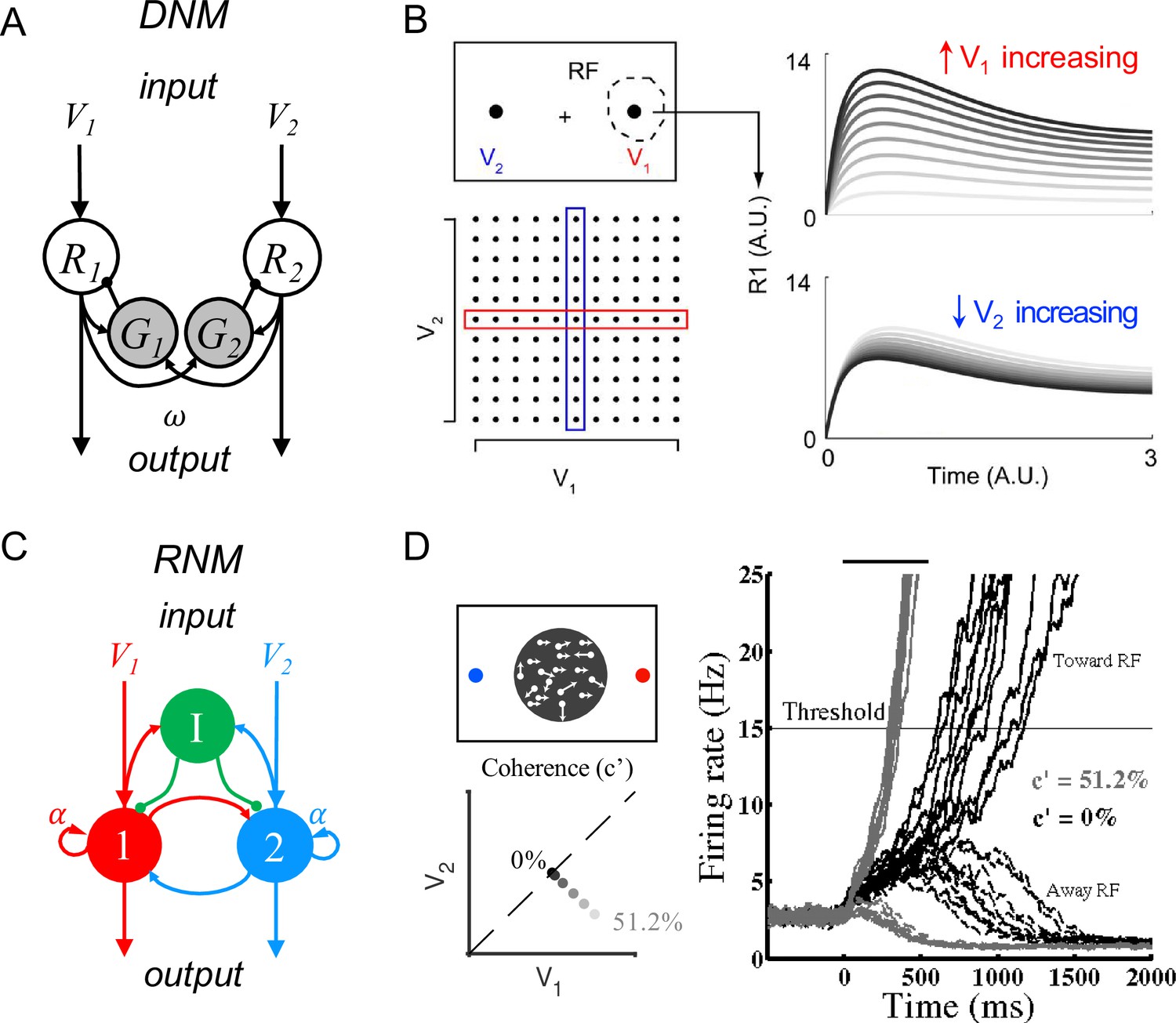
Standard circuit motifs and neural dynamics in existing decision-making models.
(A) Dynamic normalization model (DNM). Each pair of excitatory (R) and inhibitory (G) units corresponds to an option in the choice set, with R receiving value-dependent input V and providing output. Lateral interactions implement a cross-option gain control that produces normalized value coding. Panel adapted from Figure 1 from Louie et al., 2014 (B) DNM predicted dynamics replicate empirical contextual value coding. The example task involves orthogonal manipulation of both option values. R1 activity increases with the direct input value V1 (array framed in red) but is suppressed by the contextual input V2 (array framed in blue), consistent with value normalization. (C) Recurrent network model (RNM). The network consists of excitatory pools with self-excitation (1 and 2) and a common pool of inhibitory neurons (I). Panel adapted from Wong and Wang, 2006. (D) RNM predicted dynamics generate winner-take-all selection. The example task involves motion discrimination of the main direction of a random dot motion stimulus with varying coherence (c’) levels (left). Model activity (right) under two different levels of input coherence (0 and 51.2%) predicts different ramping speeds to the decision threshold and generates a selection even with equal inputs.
© 2014, Louie et al. Panel B has been reproduced from Figure 5A from Louie et al., 2014 (published under a CC BY-NC-SA 3.0 license). It is not covered by the CC-BY 4.0 license and further reproduction of this panel would need permission from the copyright holder.
© 2006, Society for Neuroscience. Panel D (right) is reproduced from Figure 2 from Wong and Wang, 2006 with permission from Society for Neuroscience. It is not covered by the CC-BY 4.0 licence and further reproduction of this panel would need permission from the copyright holder.
Figure 2 with 1 supplement
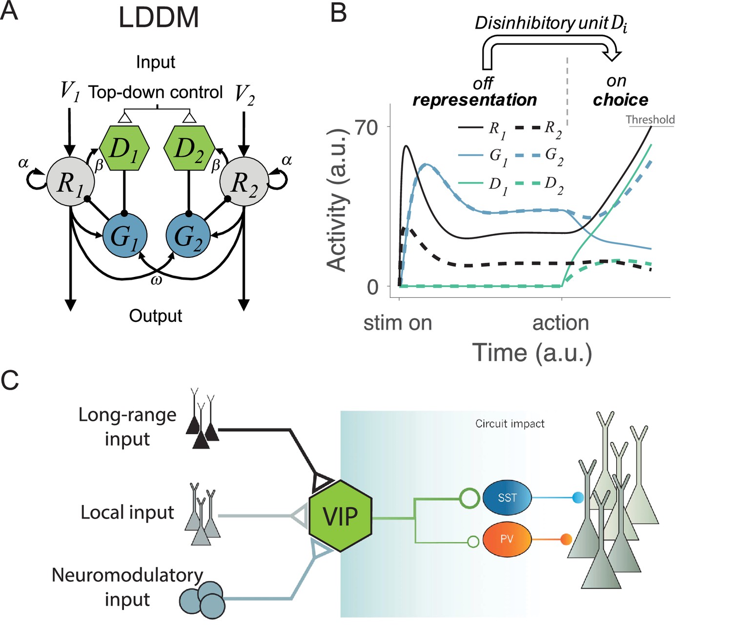
Local disinhibition decision model (LDDM) and its biological plausibility.
(A) LDDM extends the dynamic normalization model (DNM) by incorporating a disinhibitory D unit to mediate the local disinhibition of the associated excitatory R unit; strength of R to D coupling is controlled by the parameter β presumed via an external top-down control. , , and indicate the corresponding input value to each option, self-excitation of R unit, and the coupling weights from R to G unit, respectively. (B) The network phase transition between representation and choice under gated disinhibition. With the disinhibitory module silent, the network performs dynamic divisive normalization on R units and predicts non-selective inhibition via G units; after the disinhibitory module is triggered via an external top-down control signal, the network switches to a winner-take-all competition dynamic. The circuit predicts selective inhibition after disinhibition is triggered. (C) Biological basis of disinhibition. Disinhibition provides a mechanism for dynamic gating of circuit states. Vasoactive intestinal peptide (VIP)-expressing interneurons typically inhibit somatostatin (SST) and parvalbumin (PV)-positive interneurons, resulting in a disinhibition of pyramidal neurons. VIP neurons receive local, long-range, and neuromodulatory input, providing different potential mechanisms to modulate local circuit dynamics.
© 2014, Springer Nature. Panel C is reproduced from Figure 3 from Kepecs and Fishell, 2014 with permission from Springer Nature. It is not covered by the CC-BY 4.0 licence and further reproduction of this panel would need permission from the copyright holder.
Figure 2—figure supplement 1
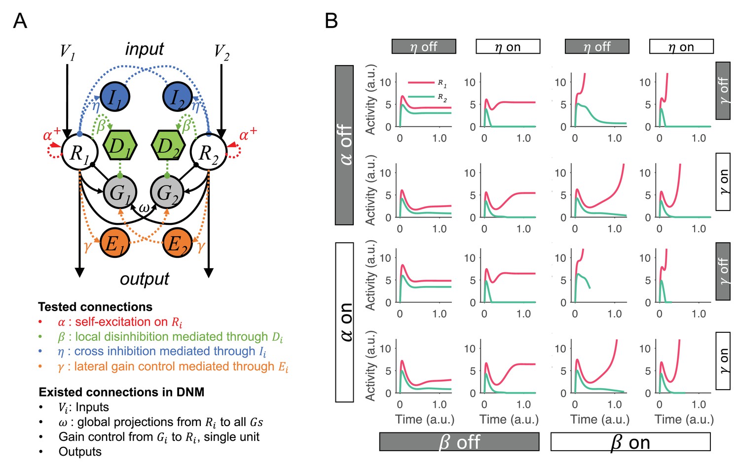
Testing and comparing different dynamic normalization model (DNM) modifications for integrating normalized value coding and winner-take-all (WTA) competition.
(A) The full model contains all possible modifications that allow the original DNM to generate WTA competition. Modifications: recurrent excitation on R units (controlled by ), local disinhibition mediated through D units (controlled by ), cross inhibition mediated throughIunits to inhibit the lateral R (controlled by ), and lateral gain control boost loops mediated through E units (controlled by ). (B) Example R1 and R2 dynamics predicted by the model variants with different combinations of modifications. Four types of modifications result in 16 candidate models. Comparing the left two columns and right two columns shows that local disinhibition () is required for generating WTA competition and increasing neural activity to a decision threshold.
Figure 3
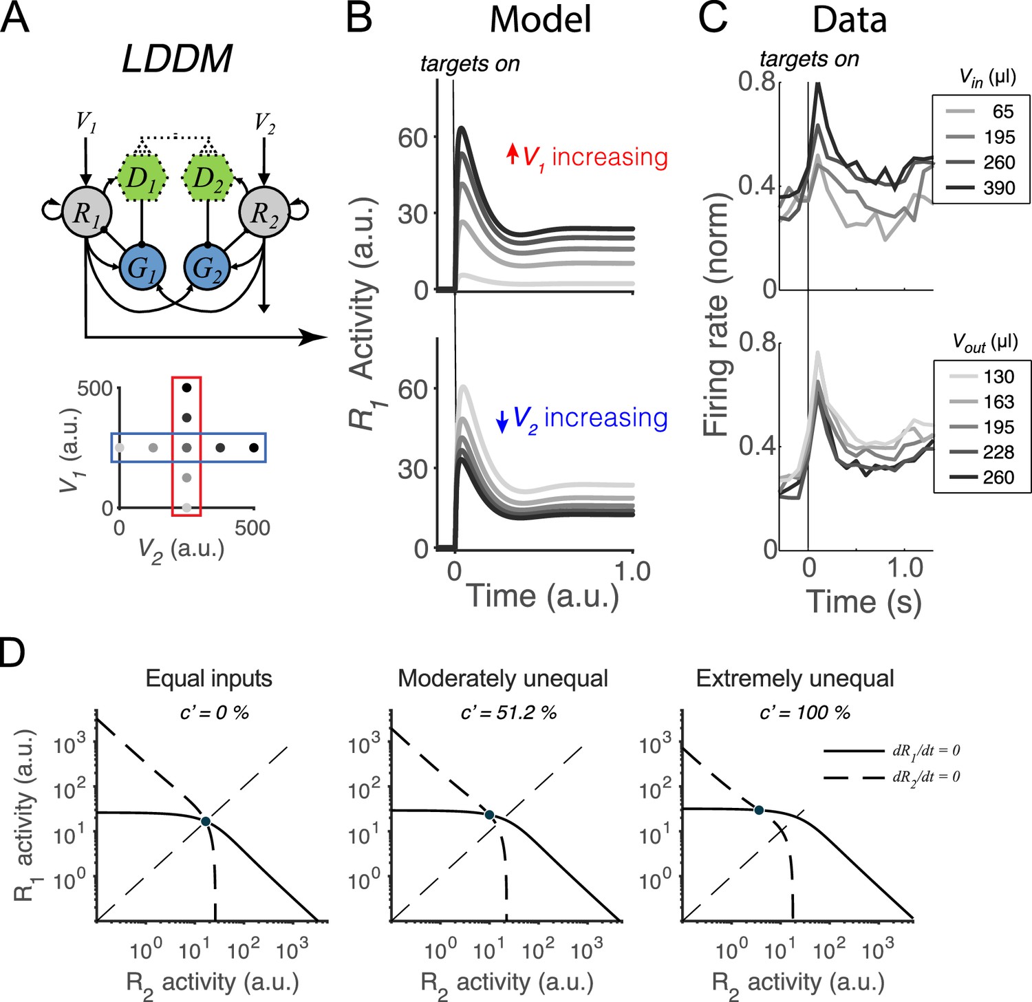
Normalized value coding in the local disinhibition decision model (LDDM).
(A) In this example, the LDDM receives a set of two input values with varying V1 (framed in red) and V2 (framed in blue). (B) Example LDDM dynamics show relative value coding. R1 activity shows a transient peak before a sustained period of coding. Increasing V1 increases R1 activity but increasing V2 decreases R1 activity. (C) Value coding dynamics recorded in monkey parietal cortex. The model prediction we showed is consistent with the empirical observation. Panel is adapted from Figure 1B and D from Louie et al., 2011. (D) Phase plane analysis of the system under equal (left), weakly unequal (middle), and extremely unequal (right) inputs. The nullclines of R1 (solid) and R2 (dashed) indicating the equilibrium state of the individual units intersect at a unique and stable equilibrium point with divisively normalized coding.
Figure 4 with 2 supplements
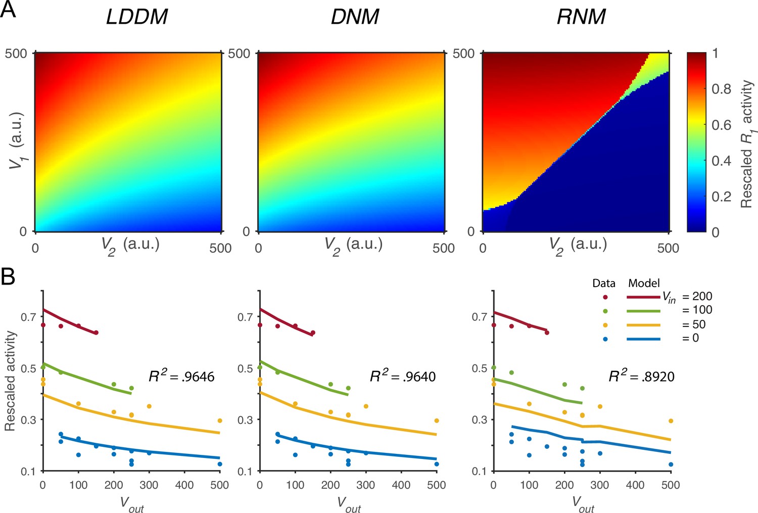
Quantitative comparison of contextual value coding across the local disinhibition decision model (LDDM), dynamic normalization model (DNM), and recurrent network model (RNM) models.
(A) Comparison between the LDDM (left), the DNM (middle), and the RNM (right) in value coding. The LDDM and the DNM show normalized value coding. The neural activity of R1 (indicated by color) increases with the direct input V1 but decreases with the contextual input V2. The LDDM shows slightly stronger contextual modulation than the DNM but qualitatively replicated normalized value coding. The RNM shows a qualitatively different pattern consistent with winner-take-all (WTA) competition. Within the regime of WTA competition (V1 and V2 within a reasonable scale), R1 activity is high when V1 > V2 and low when V1 < V2. (B) Fitting the models to a trinary choice dataset shows that the LDDM (left panel) performed slightly better than the DNM (middle panel) in capturing the neural activities responding to values inside (Vin) and outside (Vout) of the receptive field. Fitting the RNM to the dataset does not capture the neural activities as well as the LDDM (and DNM; right panel).
Figure 4—figure supplement 1
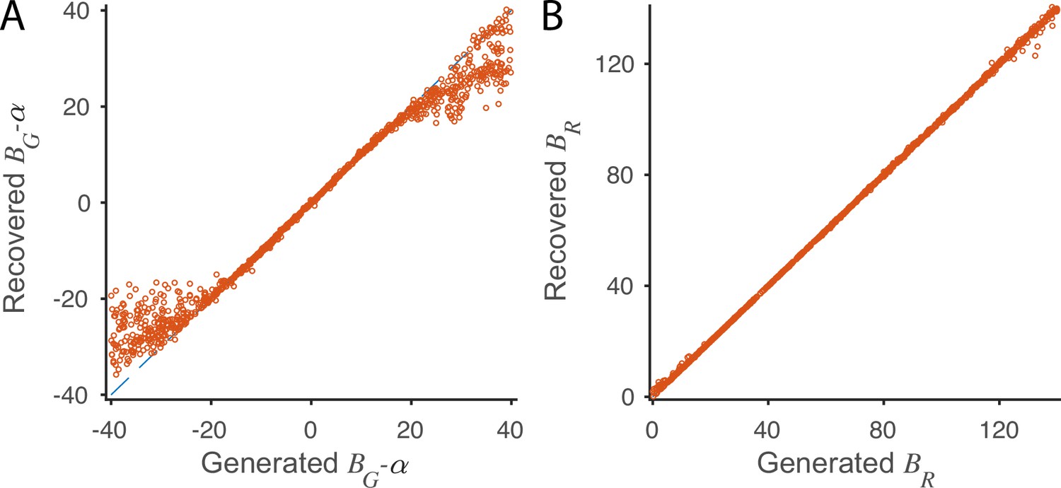
Parameter recovery in fitting the local disinhibition decision model (LDDM) to normalized value coding data.
(A) The refitted parameter as a function of the used to generate the activities during model equilibrium shows high consistency when the parameters are within a reasonable range. (B) The refitted parameter as a function of the used to generate the activities during model equilibrium shows high consistency across a wide range. When generating the model activities using the parameter located on the x-axis of each panel, other parameters were kept as the best fit in Figure 4B. A full model was refitted to the generated data on each point, and only the varying parameter was plotted in pairs with the ‘ground truth’ parameter used to generate the data.
Figure 4—figure supplement 2
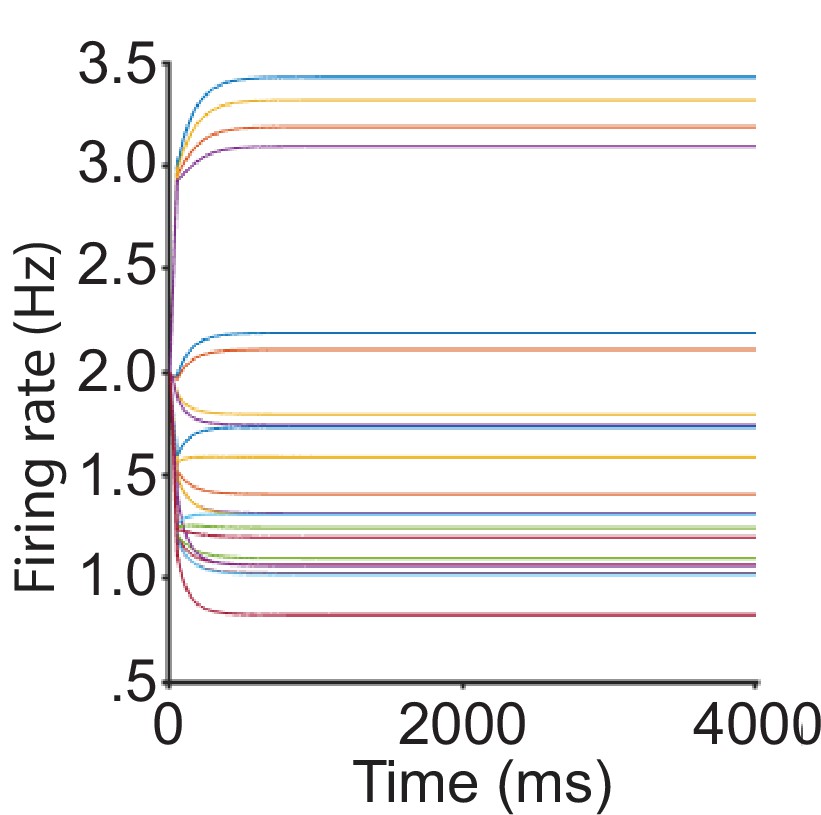
Recurrent network model (RNM) activity fit to normalized value coding data.
The predicted dynamics of neural firing rates without scaling, including the activities of all three pools across different input conditions. The predicted firing rates show an unrealistic low activity level, inconsistent with empirical observations. Note that the best-fitting parameters are no longer in a regime that generates winner-take-all competition.
Figure 5 with 1 supplement
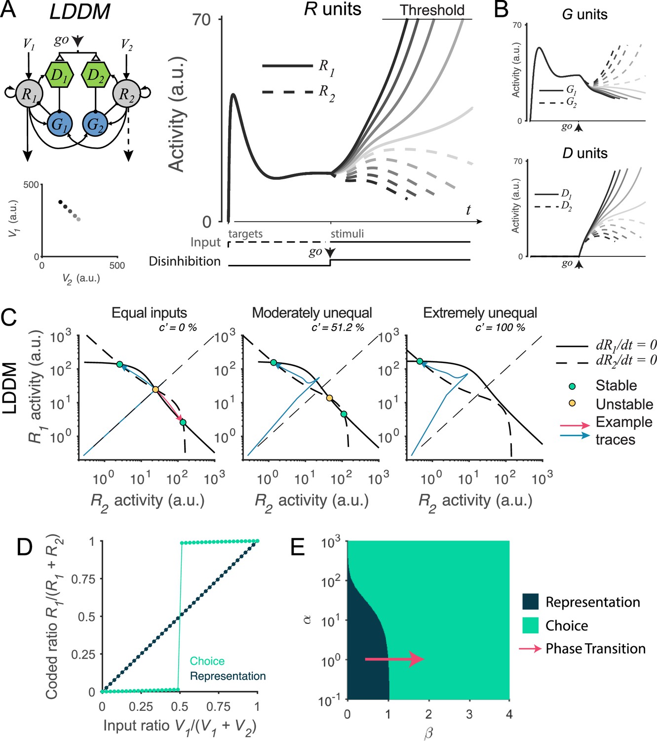
Recurrent network model (RNM)-like winner-take-all (WTA) selection dynamics in the local disinhibition decision model (LDDM).
(A) Example R1 (solid) and R2 (dashed) dynamics in a classic reaction-time motion discrimination task. The model predicts phasic stimulus onset dynamics during the pre-stimulus stage and WTA dynamics during the stimulus stage when receiving different input values (left inset). Consistent with RNM dynamics (upper right inset), the R unit receiving stronger input ramps up to reach the decision threshold while the opponent R unit activity is suppressed; the speed of bifurcation depends on the input strength. (B) The model predicted the dynamics of G units (top) and D units (bottom). (C) Phase plane analysis of the LDDM (lower) compared with the original RNM (upper inset) shows the basis for WTA dynamics under equal (left), moderately unequal (middle), and extremely unequal (right) inputs. Both models show similar features across input values: under equal inputs, the nullclines of R1 and R2 intersect on three equilibrium points, with one unstable point (yellow) and two stable attractors (green; left). Under unequal inputs, the basin of nullclines is biased to the side with stronger input (middle). When the inputs are strongly biased, only the attractor associated with stronger input retains (right). Red and blue lines show example traces of R1 and R2 activities. (D) A comparison of the coded ratio between the representation (black) and WTA competition (green) regimes. While the LDDM preserves the input ratios during value representation, it shifts to a categorical coding of choice during WTA selection. (E) Distinct normalized value coding (dark) and WTA competition (green) regimes in the parameter space defined by and . Across a wide range of , the transition between valuation and selection regimes can be implemented by an increase in (pointed by the red arrow).
Figure 5—figure supplement 1
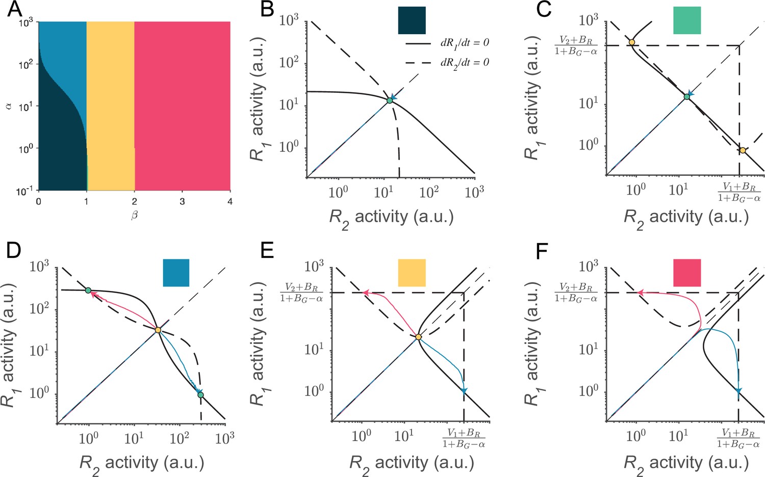
Phase plane analyses of the local disinhibition decision model (LDDM) across a wide range of recurrent excitation strengths () and local disinhibition strengths ().
(A) The five different territories in the space of and are distinguished by the patterns of equilibria and stabilities of the system. (B–F) Example nullclines of R1 (solid bold line) and R2 (dashed bold line) under each territory of parameter regime indicated by color. Nullclines intersect on equilibrium points, denoted as stable (green dots) or unstable (yellow dots). Example traces of R1 and R2 activities from equal initial values (red and green thin lines) are shown in each panel. The dark green and green regions predict normalized coding attractors but not winner-take-all (WTA) choice. The blue, yellow, and red regions predict WTA choice but have no normalized coding attractors. The vertical and horizontal dash lines indicate the predicted maximum activities when . Parameters used for visualization in these panels, (B): ; (C): ; (D): ; (E): ; (F): . Other parameters apply for all panels: , , , and .
Figure 6 with 5 supplements
The local disinhibition decision model (LDDM) performs well in capturing empirical behavior and neurophysiological data during perceptual decision-making.
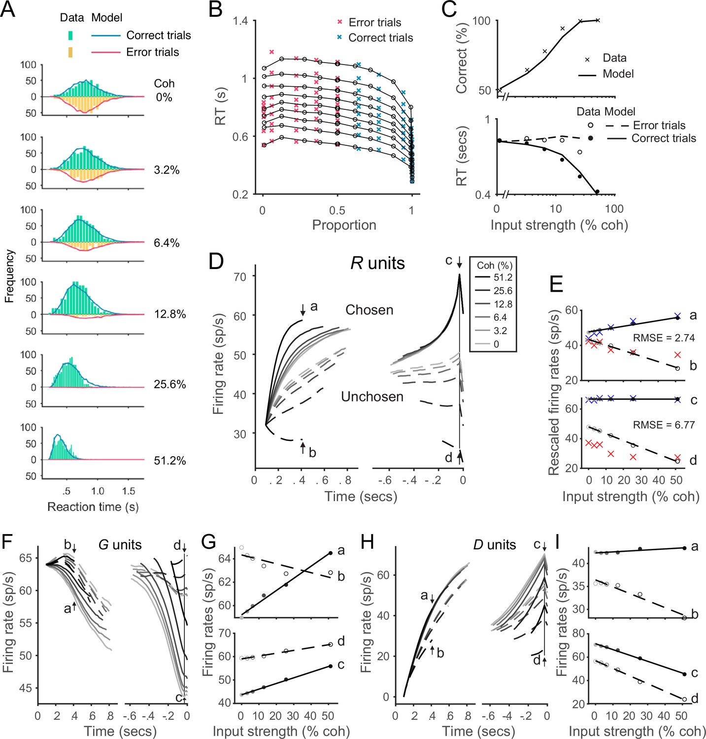
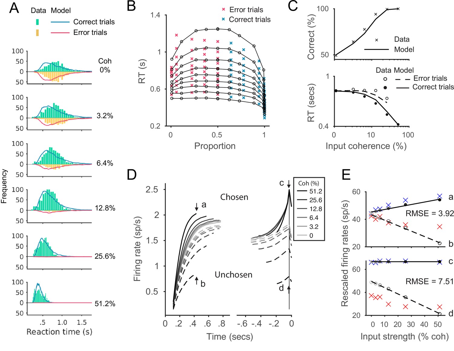
(A) Model predicted RT distributions fit to behavioral data. Predicted RT distribution (lines) match the histogram of empirical RT distribution (bars), with correct and error trials separately (indicated by color) across levels of input strength (% coherence). (B) The best-fit model predictions of the LDDM and the original recurrent network model (RNM; upper-right inset) are visualized in quantile probabilities. Nine quantiles of RT under each condition are stacked on the x-axis indicating the correct choice proportion under each input coherence (0–0.5 are error trials, shown in red crosses;.5–1 are correct trials, shown in green crosses). LDDM predicts the choice proportion and the shape of RT distribution as well as the original RNM. (C) Model predicted psychometric function (upper) and chronometric function (lower). Choice accuracy aggregated by input strength (lines) fits well to the empirical data (crosses). The predicted RT aggregated by input strength for correct (solid line) and error (dashed line) trials capture well the RT for correct (filled dots) and error (empty dots) trials in empirical data. (D) The model with best-fitting parameters to the behavior replicates the neural dynamic features of the recorded neural activity. R unit activities aligned to the onset of stimulus inputs (left) and aligned to the time of model decision (right) replicate the stereotyped ramping dynamics of units associated with the chosen side (solid lines) and suppression of units associated with the unchosen side (dashed lines) under different levels of input strength. The mean activities at the early stage (the smallest median RT of the six conditions, i.e., 410 ms after the onset of the stimulus, indicated by arrows a and b) and at the onset of model choice (indicated by arrows c and d) were examined in the following panels. (E) Quantification of the best-fit-to-behavior model prediction (dots and lines) to the empirical recordings (crosses). Upper panel: the early-stage activities at the median RT indicated by arrows a (chosen side) and b (unchosen side). Lower panel: the late-stage activities aligned to the onset of model choice (30 ms before saccade) indicated by arrows c (chosen side) and d (unchosen side). The model activities were rescaled to the threshold of the empirical activities, i.e., the mean activity across coherences indicated at arrow c. The root-mean-square error (RMSE) between the data and the model at the median RT and at the choice onset was calculated and indicated on the panels. (F) The model predicted G dynamics show a faster decreasing in the chosen units than the unchosen units, indicating that the chosen units are more strongly disinhibited. (G) Average G unit activity as a function of motion coherence at the time points indicated by letters (see panel F) for data aligned to stimulus onset (upper) and to model choice (lower). Activity is sorted by units associated with the chosen (solid lines) and unchosen (dashed lines) sides. (H) The model predicted D activities ramp in the early (dynamics on the left, sorted to the stimulus onset) and late (dynamics on the right, sorted to the choice onset) stages. (I) Average D unit activity as a function of motion coherence analogous to panel G.
Figure 6—figure supplement 1
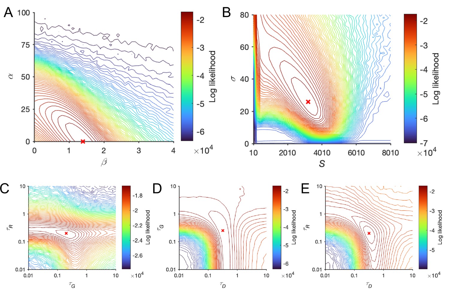
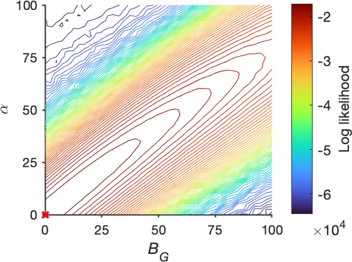
Log-likelihood surfaces for local disinhibition decision model (LDDM) fit to Roitman and Shadlen (2002) behavioral data over the regimes of the seven free parameters.
Each two parameters were paired to show the log-likelihood space, with other parameters set as the best-fitted values. The contour lines indicate the isolines of log-likelihood, with the colors indicating its value and the red cross indicating the maximized log-likelihood. The log-likelihood surfaces showed a smooth and single-point maximum topography. (A) The connection weights parameters and were paired since both control the ramping-up speed of the competition dynamics. (B) The magnitude of white noise () was paired with the magnitude of inputs (S) since these two parameters control the signal-to-noise ratio. (C–E) The time constants of the three units were paired. The values of the parameters at the maximum points precisely match the best-fitting results given the precisions of the grids (parameter values on the peaks: , , , , , (panel C) or 0.2512 (panel D; two adjacent points given the grid resolution), and ).
Figure 6—figure supplement 2
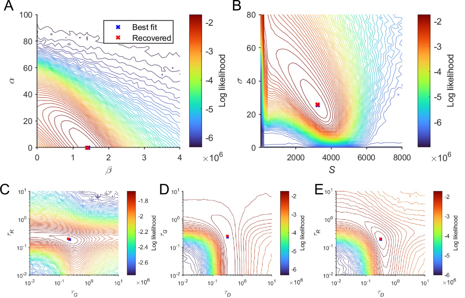
Parameter recovery of local disinhibition decision model (LDDM) for the parameters from the best fit to Roitman and Shadlen, 2002 behavioral data.
We visualized the log-likelihood of the model when re-fitting to the generated data based on the set of parameters of best fit (shown in blue crosses). Each panel shows the log-likelihood values of the model to fit the generated data across pairs of parameters. The recovered parameters (on the grid with the highest log-likelihood, indicated at red crosses) overlapped well with the parameters of best fit; the visualized discrepancy between them lies within the resolution of the grids. When the grid resolution is controlled as the same, the recovered parameters in the current figure are exactly the same as in Figure 6—figure supplement 1, indicating that the parameters are recoverable and identifiable (, , , , , [panel C] or 0.2512 [panel D; two adjacent points given the grid resolution],and ).
Figure 6—figure supplement 3
Collinearity between self-excitation and baseline gain control .
The log-likelihood space showed high collinearity between and Other parameters were set as the best-fitting values shown in Figure 6.
Figure 6—figure supplement 4
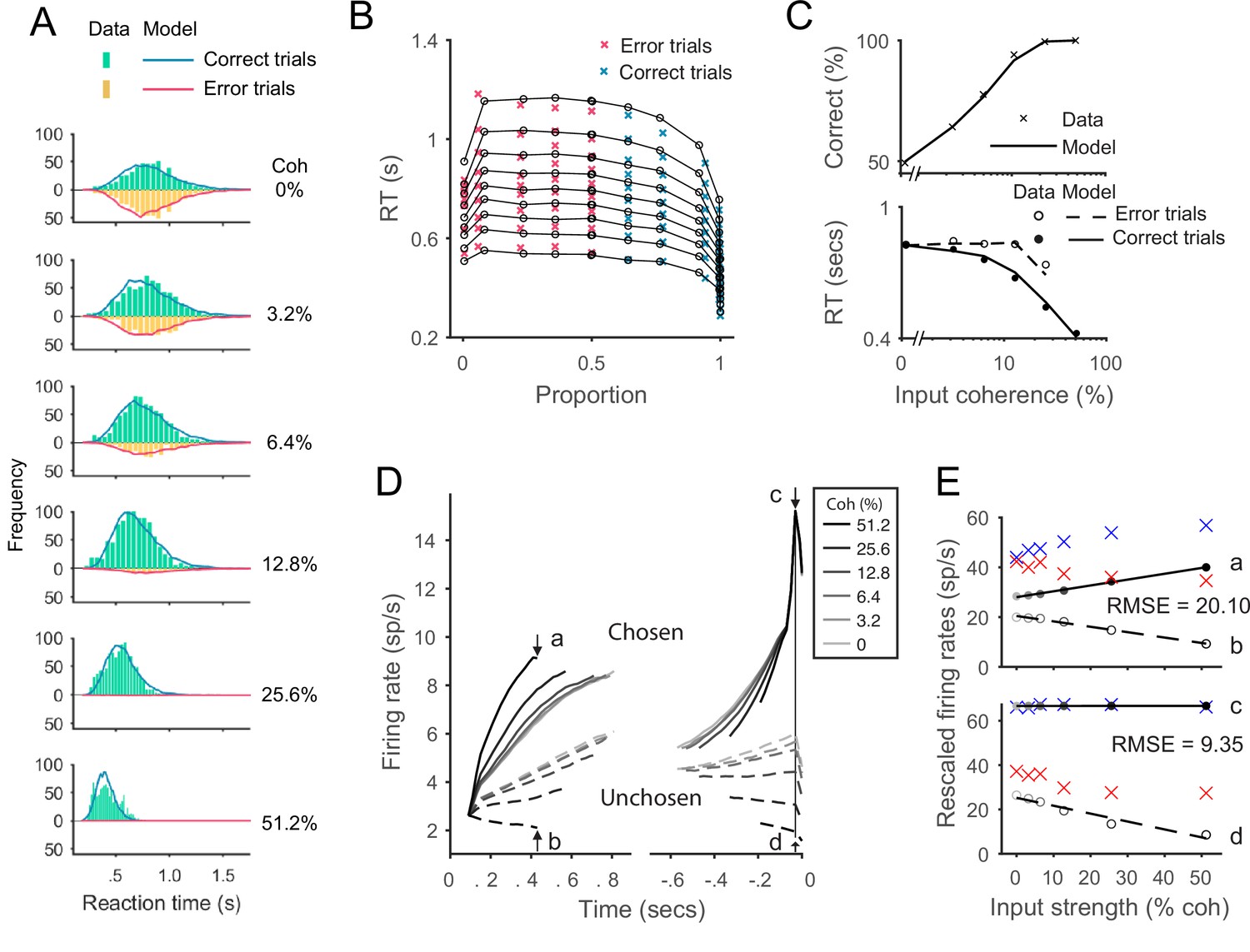
Fit of the original recurrent network model (RNM) to Roitman and Shadlen, 2002 behavioral data with eight free parameters.
All legends are consistent with the corresponding panels in Figure 6. (A) Model predicts RT distributions (lines) are slightly more right-skewed than the empirical RT distribution (histograms). (B) Visualization of the fitting results in quantile probabilities shows that the fitted third to sixth quantile lines (counting upwards from the bottom) were slightly deviated from the data points. (C) The model predicted average values of RT and choice accuracy still captured well the empirical averages. (D) The aggregated neural dynamics from the best fitting parameters of RNM. Left, mean-field activities on the excitatory pools aligned to the onset of stimulus inputs. The ramping-up speeds differ over input strengths (see the detailed pattern in E). Right, mean-field activities on the excitatory pools aligned to the time of choice execution. The unchosen signals show graded coding of the input strengths (see the detailed pattern in E). The activities at the time point of the smallest median RT of the six conditions (430 ms after stimulus onset, indicated by arrows a and b) and at the onset of model choice (indicated by arrows c and d) were examined in the following panels. (E) Quantification of the rescaled model activities (dots and lines) to the empirical data (crosses). Upper panel: the activities of the chosen units (a) and the unchosen units (b) at the median RT. Lower panel: the activities of the chosen units (c) and unchosen units (d) at the choice onset. The model activities were rescaled to the empirical threshold, i.e., mean value across conditions at the time point indicated by arrow c. The root-mean-square error (RMSE) at the median RT and choice onset were calculated and indicated on the panels. The best-fitting parameters were self-excitation , mutual inhibition , non-selective input , noise amplitude , input scale , synaptic kinetic parameter , initial value , and the time constant of the excitatory units .
Figure 6—figure supplement 5
Fit of the leaky competing accumulator (LCA) model to Roitman and Shadlen, 2002 behavioral data, with four free parameters (Usher and McClelland, 2001).
All legends were kept consistent with the corresponding panels in Figure 6. (A) Model predicts RT distributions (lines) were slightly more right-skewed than the empirical data histogram (bars). (B) Re-plot the fitting results in quantile probabilities. The predicted RTs are slightly shorter than the empirical data at the first to sixth quantile lines, while slightly longer at the eighth and nine quantiles. (C) Model predicted mean RTs and accuracy matched well with the empirical data. (D) The aggregated neural dynamics from the best fitting parameters of LCA. The dynamics sorted to the onset of the stimulus (left) and sorted to the onset of choice (right) behave similarly to the predictions from local disinhibition decision model (LDDM) and recurrent network model (RNM). The mean activities at the smallest median RT of the six conditions (430 ms after stimulus onset; indicated by arrows a and b) and at the time of model choice (indicated by arrows c and d) were examined in the following panel. (E) Quantification of the rescaled model activities (dots and lines) to the empirical data (crosses). Upper panel: the activities of the chosen units (a) and the unchosen units (b) at the median RT. Lower panel: the activities of the chosen units (c) and unchosen units (d) at the choice onset. The model activities were rescaled to the empirical threshold, i.e., mean value across conditions at the time point indicated by arrow c. The root-mean-square error (RMSE) at the median RT and choice onset were calculated and indicated on the panels. The best-fitting parameters were leaky parameter , lateral inhibition , noise , and ; non-decision delay was fixed as 120 ms, the same as in the other models.
Figure 7
Local disinhibition decision model (LDDM) replicates both the normalized coding and winner-take-all (WTA) competition observed sequentially in single neurons examined in a multi-alternative choice task.
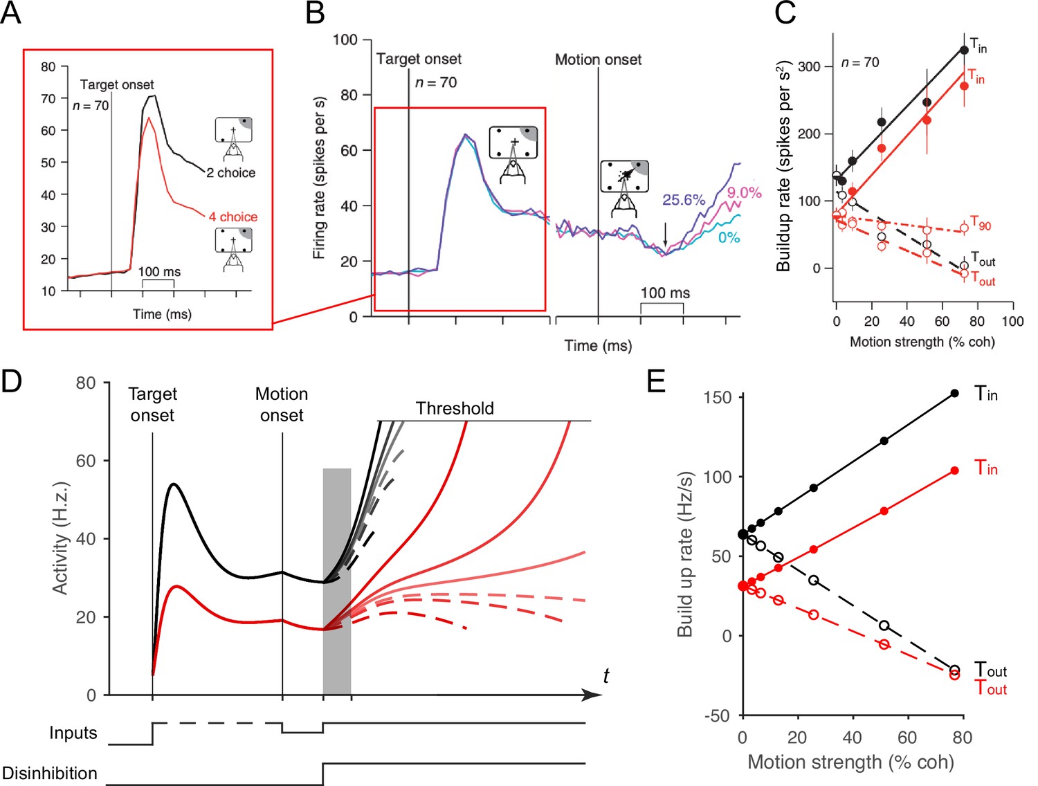
(A) Parietal neuron activity during pre-motion representation is decreased in four-alternative (red) versus two-alternative (black) trials. (B) Neural activity during two-alternative choice transitions from pre-motion target representation (left) and to post-motion onset WTA dynamics (right), shown for different input coherences (indicated by colors). (C). Ramping speed in two (black) and four (red) alternative conditions, separated for choices toward (Tin) and away from (Tout) the neural response field (T90 in the original study designates choices for targets orthogonal to the Tin-Tout target, and is not examined here). (D) Dynamics of LDDM R unit activity during pre-motion representation without disinhibition (left) and after motion onset with disinhibition (right). (E) LDDM replicates the decrease in ramping rates (time period shaded in D) from two (black) to four (red) alternatives after the motion onset, consistent with the empirical data.
© 2008, Springer Nature. Panels A-C are reprinted from Figures 3B, 2C and 4F, respectively, from Churchland et al., 2008, with permission from Springer Nature. These are not covered by the CC-BY 4.0 license, and further reproduction of these panels would need permission from the copyright holder.
Figure 8 with 2 supplements
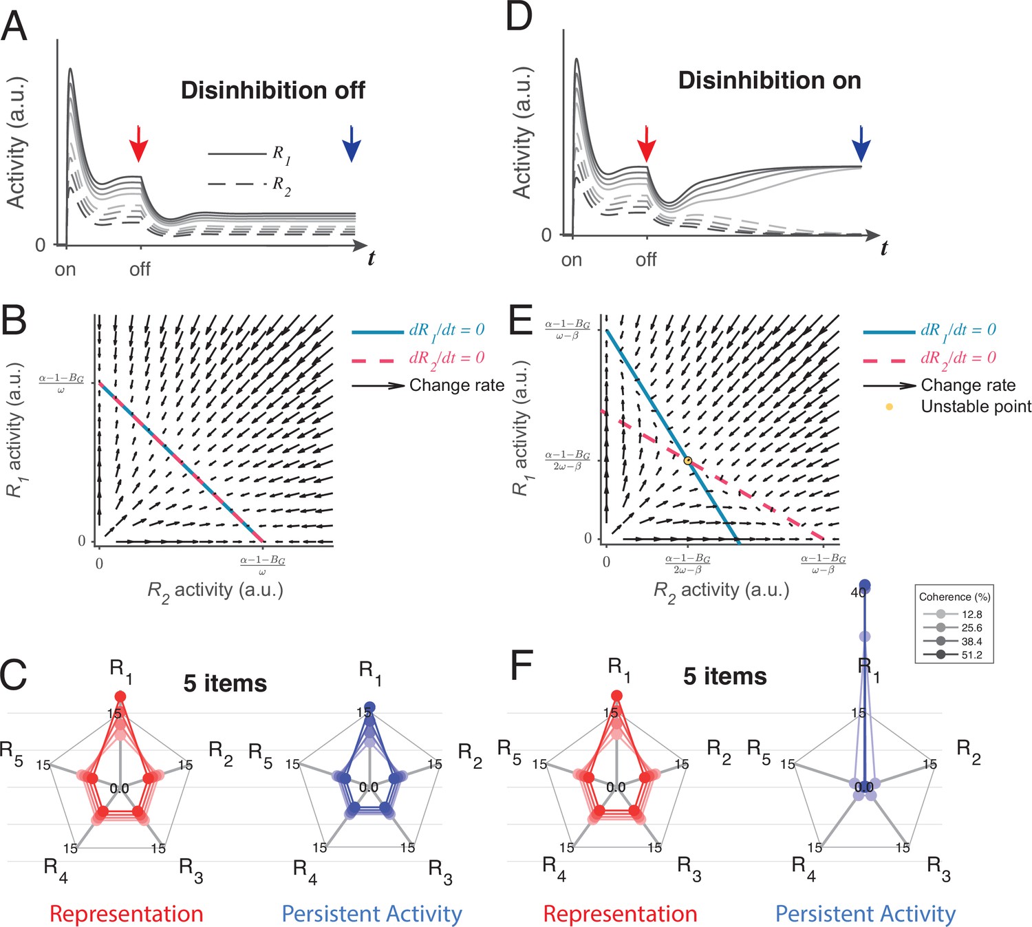
Local disinhibition decision model (LDDM) disinhibition controls the flexible implementation of either line attractor or point attractor dynamics in persistent activity.
(A–C) LDDM under silent disinhibition preserves the input ratio information during persistent activity. (A) Example R1 (solid) and R2 (dashed) activities before and after withdrawal of stimuli under different levels of inputs. Neural activity decreases after withdrawal but reaches a new steady that preserves the graded coding of the inputs. (B) Phase plane analysis of persistent activity exhibits a line attractor under inactivated disinhibition. The nullclines of R1 (blue) and R2 (red) intersect on the line of attractors, on which the summed value of R activities is a constant (). Red arrows indicate the instantaneous change rate of R1 and R2 at given initial values, following the direction that preserves the R1–R2 ratio. (D–F) Persistent activity under active disinhibition preserves only the largest item as categorical information. (D) Example R1 and R2 activities before and after withdrawal of stimuli. Disinhibition activates at the same time as the offset of stimuli. During the delay period, the activity dynamic gradually switches from a graded coding of the inputs to a winner-take-all (WTA) type of categorical coding, preserving only the larger item. (E) Delay period phase plane analysis exhibits a point-attractor state under activated disinhibition. The nullclines of R1 (blue) and R2 (red) intersect on an unstable point. Red arrows indicating the instantaneous change rate of R1 and R2 bifurcate from the middle to the side corners, resulting in a high-contrast categorical coding. (C and F) Expansion of the LDDM from a two-item circuit to a five-item circuit, under inactivation and activation of disinhibition. Each axis on the radar plot indicates the activity of one R unit. Dots connected with a line indicate the R activities under the same input conditions. The input values change according to coherence level (c’) as S*[1+c’] for R1 and S* [1-c’] for R2 to R5. Representation before the withdrawal of inputs (left panels in C and F) and persistent activity without disinhibition (right panel in C) preserve the information about the input values. While persistent activity under disinhibition (right panel in F) only preserves the item that received the largest input, with activities of the other items suppressed.
Figure 8—figure supplement 1
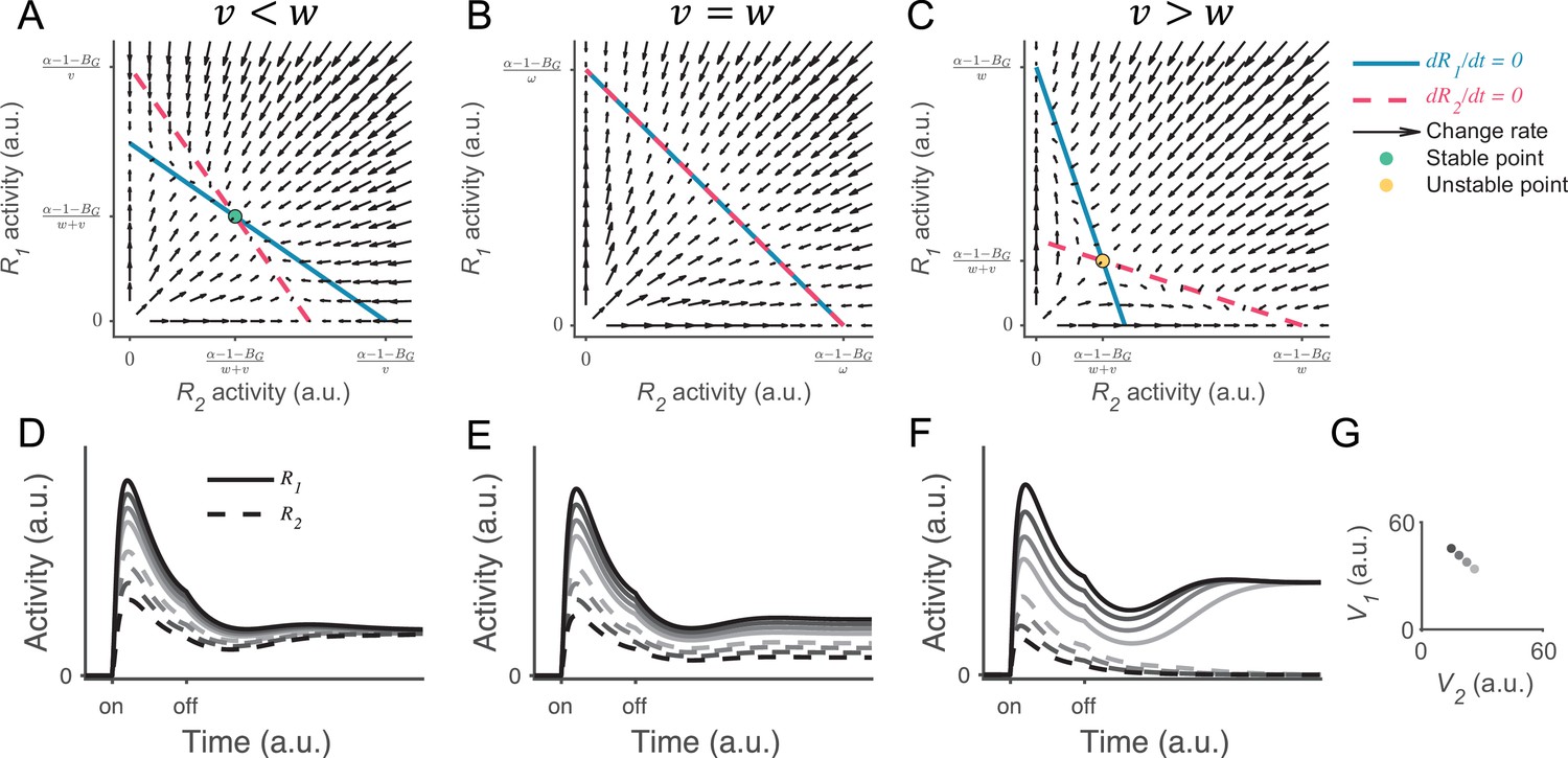
Analysis of local disinhibition decision model (LDDM) persistent activity under generalized gain control weights.
(A–C) Phase plane analysis shows that systems with different gain control weights have different patterns of equilibria and stabilities. (A) When the lateral gain control () is weaker than the local gain control (), the nullclines of R1 (blue solid) and R2 (red dashed) intersect on an attractive unique equilibrium point. The vector filed (red arrows) indicates the instantaneous change rate of R1 and R2 at given initial values. Any initial values converge into the equilibrium point, with R1 and R2 sharing the same value . (B) When , the nullclines of R1 and R2 overlap on the line of attraction. The vector field shows that any initial values converge onto the line of attraction along the direction that preserves the original input ratio. (C) When , the nullclines of R1 and R2 intersect on a unique but unstable point. Any initial values diverge from the point and bias to the side with the higher initial value, realizing winner-take-all (WTA) competition. (D–F) Example neural dynamic on R1 and R2 when under different input ratios (indicated by grayscale and shown in G). Corresponding to the phase plane analysis in A–C, the activities of R1 and R2 gradually converge onto the same value when , keep the input ratio when , and diverge based on the input ratio when . (G). Input values used in the simulations.
Figure 8—figure supplement 2
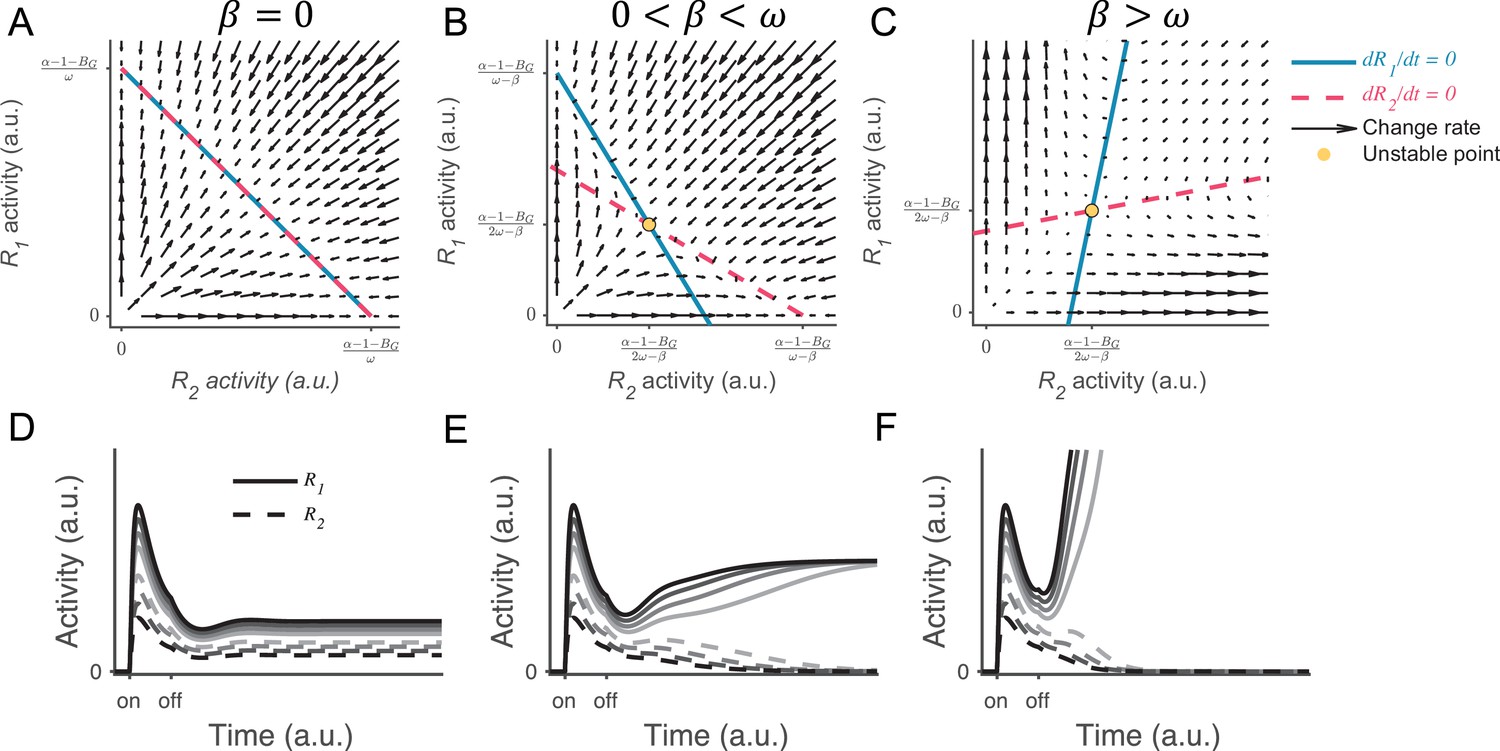
Local disinhibition decision model (LDDM) persistent activity under different levels of local disinhibition.
(A–C) Phase plane analysis of persistent activity for the situations of inactive disinhibition (, A), moderate intensity of disinhibition (, B), and strong disinhibition (, C). When , the nullclines of R1 (blue solid) and R2 (red dashed) intersect on a line of attraction, resulting in normalized value coding. When and , the R1 and R2 nullclines intersect on an unstable repellor. The vector field (red arrows) shows the instantaneous change rate of R1 and R2 at given initial values. (D–F) Example R1 and R2 dynamics under different input values (indicated by grayscale in Figure 8—figure supplement 1). When (D), the activities of R1 (solid) and R2 (dashed) maintain the normalized coding of input values during persistent activity. When (E), R1 and R2 gradually transition from coding of the normalized value to coding of categorical choice, but the activity is still beneath the decision threshold. When (F), R1 and R2 exhibit winner-take-all (WTA) dynamics, and the winner reaches the decision threshold.
Figure 9
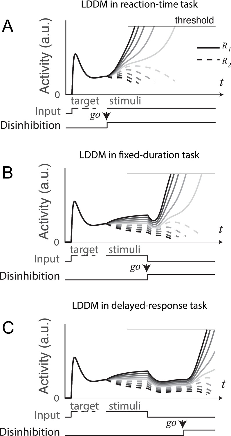
Gated disinhibition flexibly adapts the dynamics of the circuit to various types of tasks.
All of the tasks consist of a pre-stimulus stage with equal inputs to R1 (solid) and R2 (dashed) and a stimulus stage with input values determined by the stimuli (indicated by grayscale, the same value matrix as used in Figure 5A). (A) Reaction-time task. Subjects are free to respond at any time following stimulus onset, and model disinhibition is activated with the onset of stimuli. Model dynamics show winner-take-all (WTA) competition right after the onset of stimuli. (B) Fixed duration task. Subjects are required to wait for a fixed duration of stimulus viewing before choice, and model disinhibition is turned on only at the onset of the instruction cue (usually indicated in experiments by fixation point offset). Model dynamics show normalized value coding before the instruction cue and a transition to WTA choice afterward. (C) Working memory (delayed response) task. Subject choice occurs after an interval of stimulus presentation and a subsequent delay interval without stimuli, and model disinhibition is turned on at the end of the delay period. Model dynamics exhibit normalized value coding during stimulus input, preserved relative value information during the delay period, and a transition to WTA choice dynamic after the instruction cue.
Figure 10
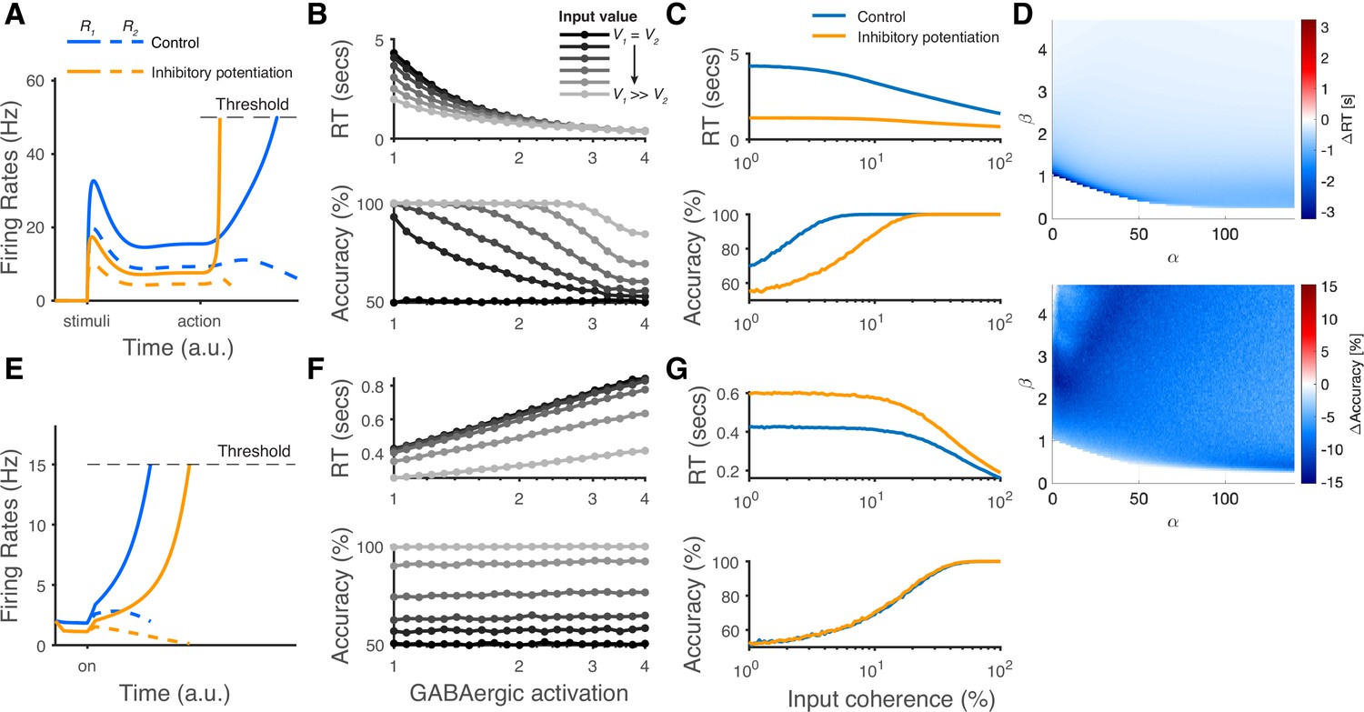
The modeling predictions of inhibitory potentiation to decision-making neural dynamics and behaviors.
(A) The predicted neural dynamics of pyramidal neurons (R1, solid lines, and R2, dashed lines) activities in a fixed duration decision task from local disinhibition decision model (LDDM). The inhibitory potentiation condition (orange) compared to the control condition (blue) decreases neural activities during early-stage representation but speeds up winner-take-all (WTA) bifurcation during choice. (B) Increasing the levels of Inhibitory potentiation speeds up RTs but decreases choice accuracy, examined over multiple levels of input coherences (indicated by grayscales). (C) Comparing inhibitory potentiation (orange) with control (blue), the differences will be evident in average chronometric and psychometric curves. (D) The predicted behavioral pattern can be generalized across the full space of and parameters regime in the LDDM. (E) The predicted neural dynamics of primary neurons (R1, solid lines, and R2, dashed lines) activities from recurrent network models (RNMs; e.g. Wong and Wang, 2006). Since the model does not include a mechanism of switch, the fixed duration task is not able to be tested in this type of model. We examined the reaction time task instead. RNM predicts suppressed neural dynamics under inhibitory potentiation. (F) RNM predicts increased RTs but unchanged accuracy. (G) The chronometric and psychometric curves predicted by RNM will be qualitatively different from LDDM.
Author response image 1
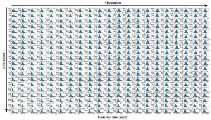
The shape of predicted reaction-time distribution over a wide range of α and β values by LDDM.
Each grid indicates the predicted RT histogram normalized in the range of minimum and maximum RTs. The shape of RT distribution exhibits a pattern of increasing skewness when α increases and decreasing skewness when β increases.
Additional files
Download links
A two-part list of links to download the article, or parts of the article, in various formats.
Downloads (link to download the article as PDF)
Open citations (links to open the citations from this article in various online reference manager services)
Cite this article (links to download the citations from this article in formats compatible with various reference manager tools)
Flexible control of representational dynamics in a disinhibition-based model of decision-making
eLife 12:e82426.
https://doi.org/10.7554/eLife.82426


