Figures and data in Rapid protein stability prediction using deep learning representations

Figures
Tables
Additional files

5 figures, 4 tables and 1 additional file

Figures

Figure 1

Download asset Open asset

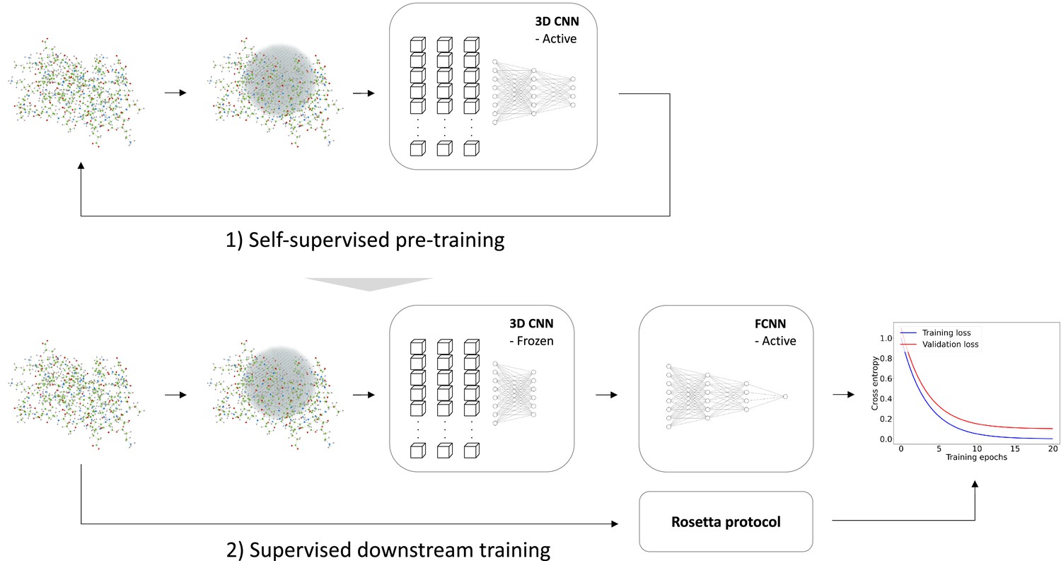
Overview of model training.

We trained a self-supervised three-dimensional convolutional neural network (CNN) to learn internal representations of protein structures by predicting wild-type amino acid labels from protein structures. The representation model is trained to predict amino acid type based on the local atomic environment parameterized using a 3D sphere around the wild-type residue. Using the representations from the convolutional neural network as input, a second downstream and supervised fully connected neural network (FCNN) was trained to predict Rosetta $Δ Δ G$ values.

Figure 2 with 3 supplements

Download asset Open asset

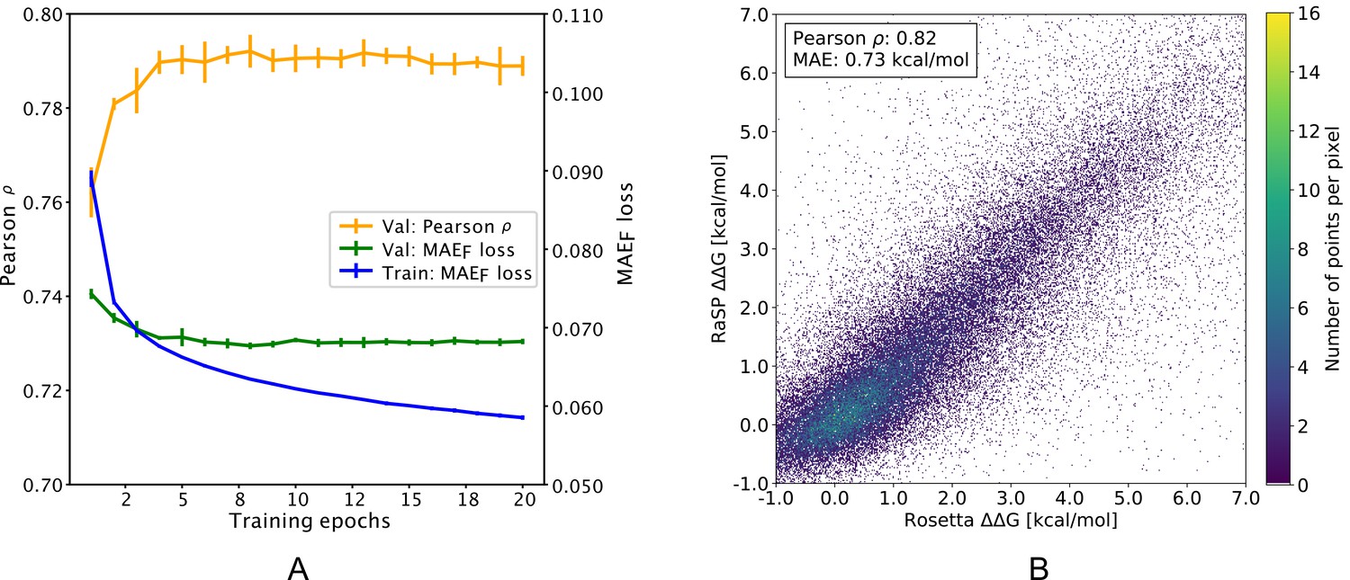
Overview of RaSP downstream model training and testing.

(A) Learning curve for training of the RaSP downstream model, with Pearson correlation coefficients ( $ρ$ ) and mean absolute error ( ${MAE}_{F}$ ) of RaSP predictions. During training we transformed the target $Δ Δ G$ data using a switching (Fermi) function, and ${MAE}_{F}$ refers to this transformed data (see Methods for further details). Error bars represent the standard deviation of 10 independently trained models, that were subsequently used in ensemble averaging. Val: validation set; Train: training set. (B) After training, we applied the RaSP model to an independent test set to predict $Δ Δ G$ values for a full saturation mutagenesis of 10 proteins. Pearson correlation coefficients and mean absolute errors (MAE) were for this figure computed using only variants with Rosetta $Δ Δ G$ values in the range [–1;7] kcal/mol.

Figure 2—figure supplement 1

Download asset Open asset

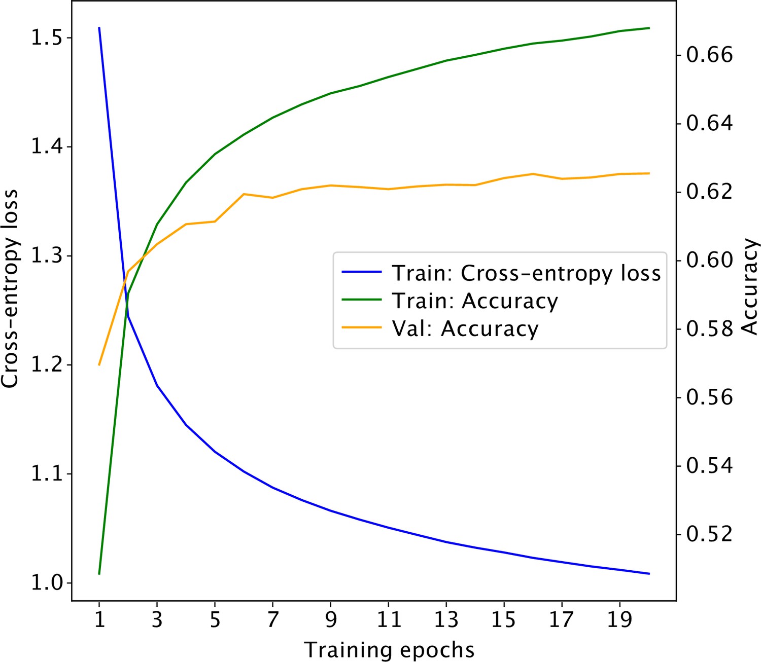
Learning curve for the self-supervised 3D convolutional neural network.

The model obtained at epoch 15 achieves a classification accuracy of 63% on the validation set.

Figure 2—figure supplement 2

Download asset Open asset

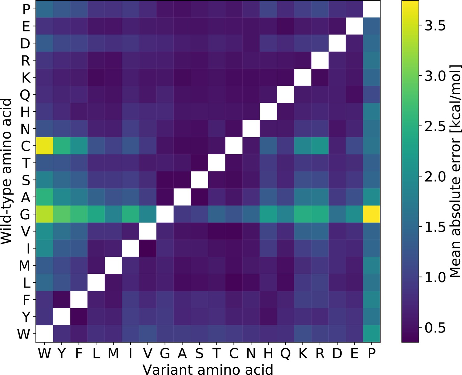
Mean absolute prediction error for RaSP on the validation set, split by amino acid type of the wild-type and variant residue.

Substitutions from glycine and cysteine as well as to proline generally have higher errors.

Figure 2—figure supplement 3

Download asset Open asset

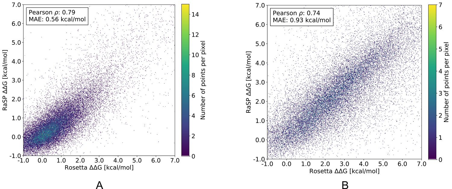
RaSP versus Rosetta $Δ Δ G$ values for a full saturation mutagenesis of 10 test proteins separated into either exposed (A) or buried (B) residues.

We speculate, that the RaSP prediction task is harder in the case of buried residues because Rosetta $Δ Δ G$ values generally have higher variance in those regions. Pearson correlation coefficients and mean absolute errors (MAE) were for this figure computed using only variants with Rosetta $Δ Δ G$ values in the range [–1;7] kcal/mol. Buried and exposed residue were classified based a relative surface accessible surface area (SASA) cut-off of 0.2.

Figure 3 with 4 supplements

Download asset Open asset

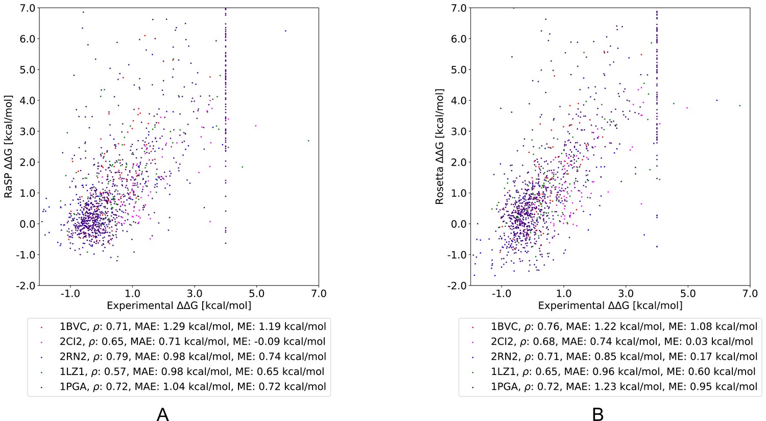
Comparing RaSP and Rosetta predictions to experimental stability measurements.

Predictions of changes in stability obtained using (A) RaSP and (B) Rosetta are compared to experimental data on five test proteins; myoglobin (1BVC), lysozyme (1LZ1), chymotrypsin inhibitor (2CI2), RNAse H (2RN2) and Protein G (1PGA) (Kumar, 2006; Ó Conchúir et al., 2015; Nisthal et al., 2019). Metrics used are Pearson correlation coefficient ( $ρ$ ), mean absolute error (MAE) and mean error (ME). In the experimental study of Protein G, 105 variants were assigned a $Δ Δ G$ value of at least 4 kcal/mol due to low stability, presence of a folding intermediate, or lack expression (Nisthal et al., 2019).

Figure 3—figure supplement 1

Download asset Open asset

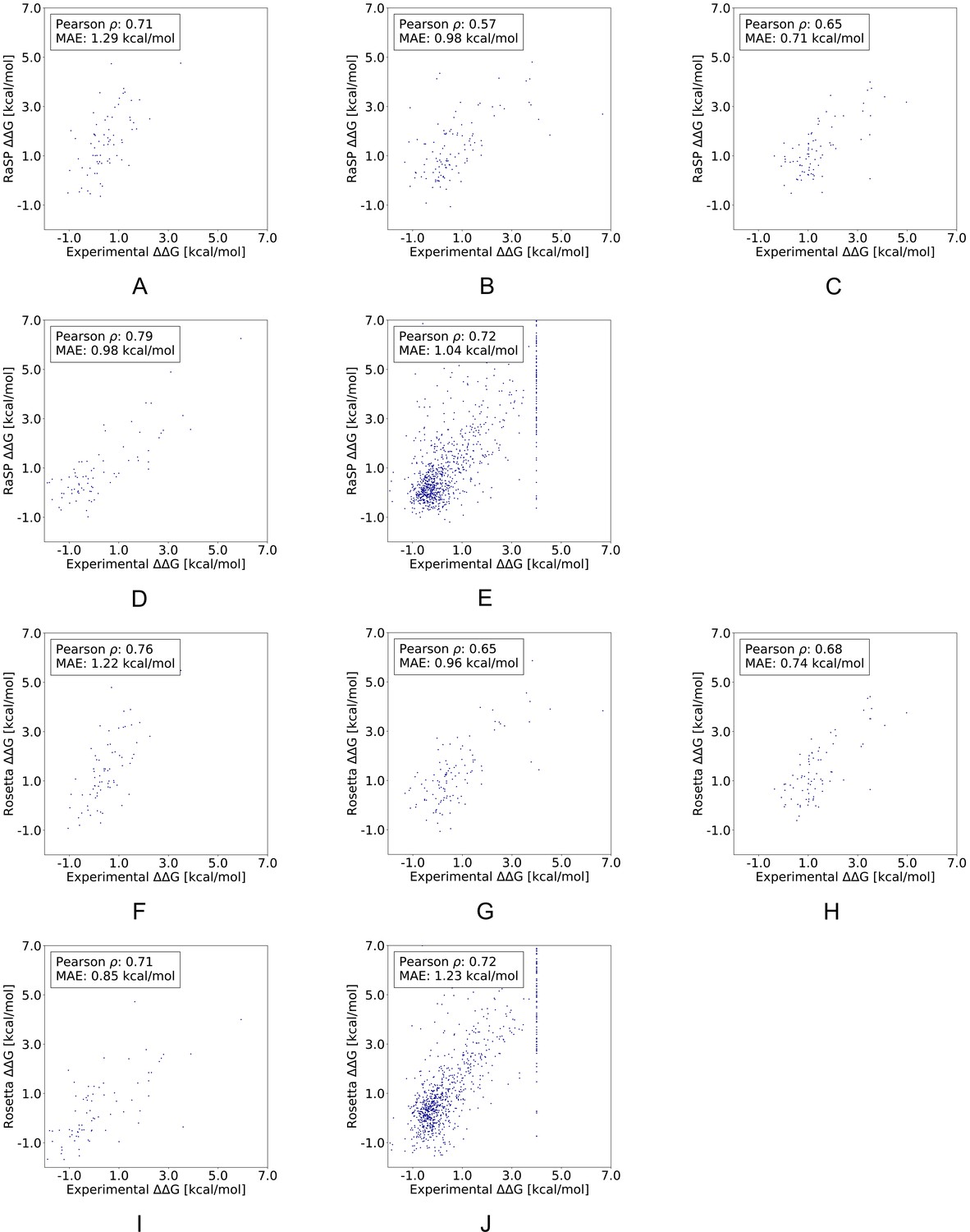
Comparing RaSP and Rosetta predictions to experimental stability measurements.

Stability predictions obtained using (A–E) RaSP and (F–J) Rosetta are compared to experimental data for the five test proteins; myoglobin (1BVC), lysozyme (1LZ1), chymotrypsin inhibitor (2CI2), RNAse H (2RN2) and Protein G (1PGA) (Kumar, 2006; Ó Ó Conchúir et al., 2015; Nisthal et al., 2019). In the experimental study of Protein G, 105 variants were assigned a $Δ Δ G$ value of at least 4 kcal/mol due to low stability, presence of a folding intermediate, or lack expression (Nisthal et al., 2019).

Figure 3—figure supplement 2

Download asset Open asset

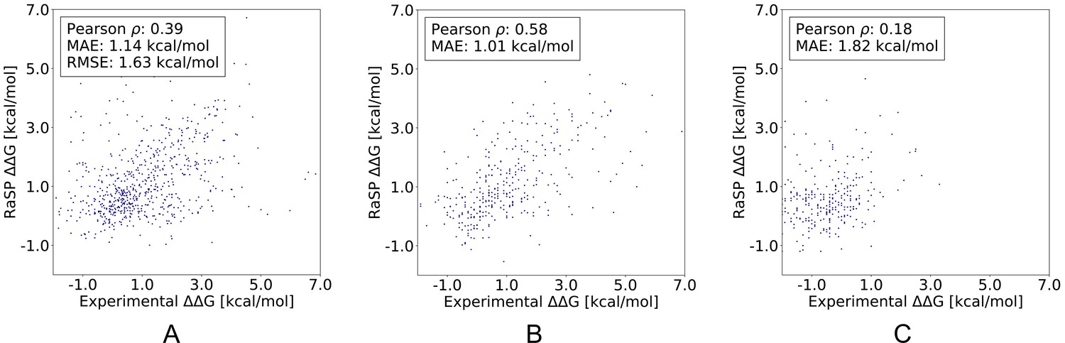
RaSP performance on three recently published data sets (Pancotti et al., 2022): (A) The S669 data set, (B) The Ssym+ direct data set, (C) The Ssym+ reverse data set.

Figure 3—figure supplement 3

Download asset Open asset

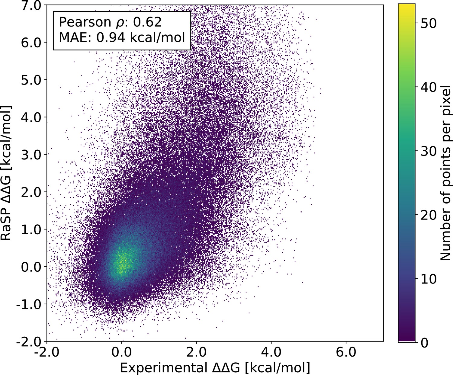
RaSP performance on the recently published mega-scale experiments (Tsuboyama et al., 2022).

The experimental data has been filtered to include only well-defined experimental $Δ Δ G$ values from single substitution mutations in natural protein domains (Tsuboyama et al., 2022). This filtered data set contains a total of 164,524 variants across 164 protein domain structures.

Figure 3—figure supplement 4

Download asset Open asset

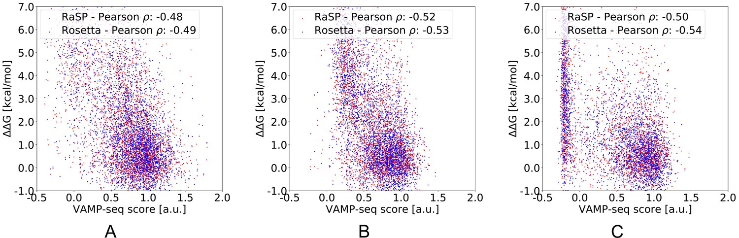
Benchmarking RaSP and Rosetta using VAMP-seq data.

We compare stability predictions with VAMP-seq scores for three test proteins (A) TPMT (PDB: 2H11) (Matreyek et al., 2018), (B) PTEN (PDB: 1D5R) (Matreyek et al., 2018) and (C) NUDT15 (PDB: 5BON) (Suiter et al., 2020).

Figure 4

Download asset Open asset

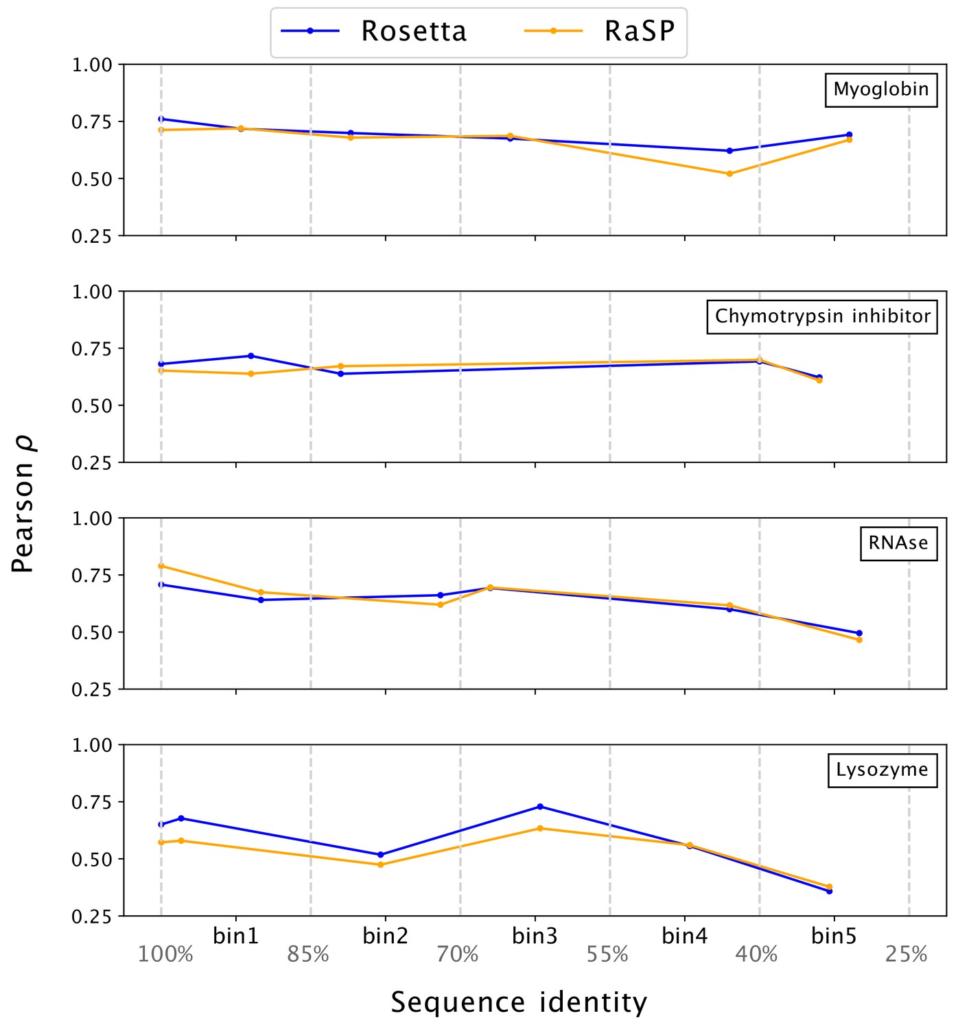
Stability predictions from structures created by template-based modelling.

Pearson correlation coefficients ( $ρ$ ) between experimental stability measurements and predictions using protein homology models with decreasing sequence identity to the target sequence. Pearson correlation coefficients were computed in the range of [–1;7] kcal/mol.

Figure 5 with 3 supplements

Download asset Open asset

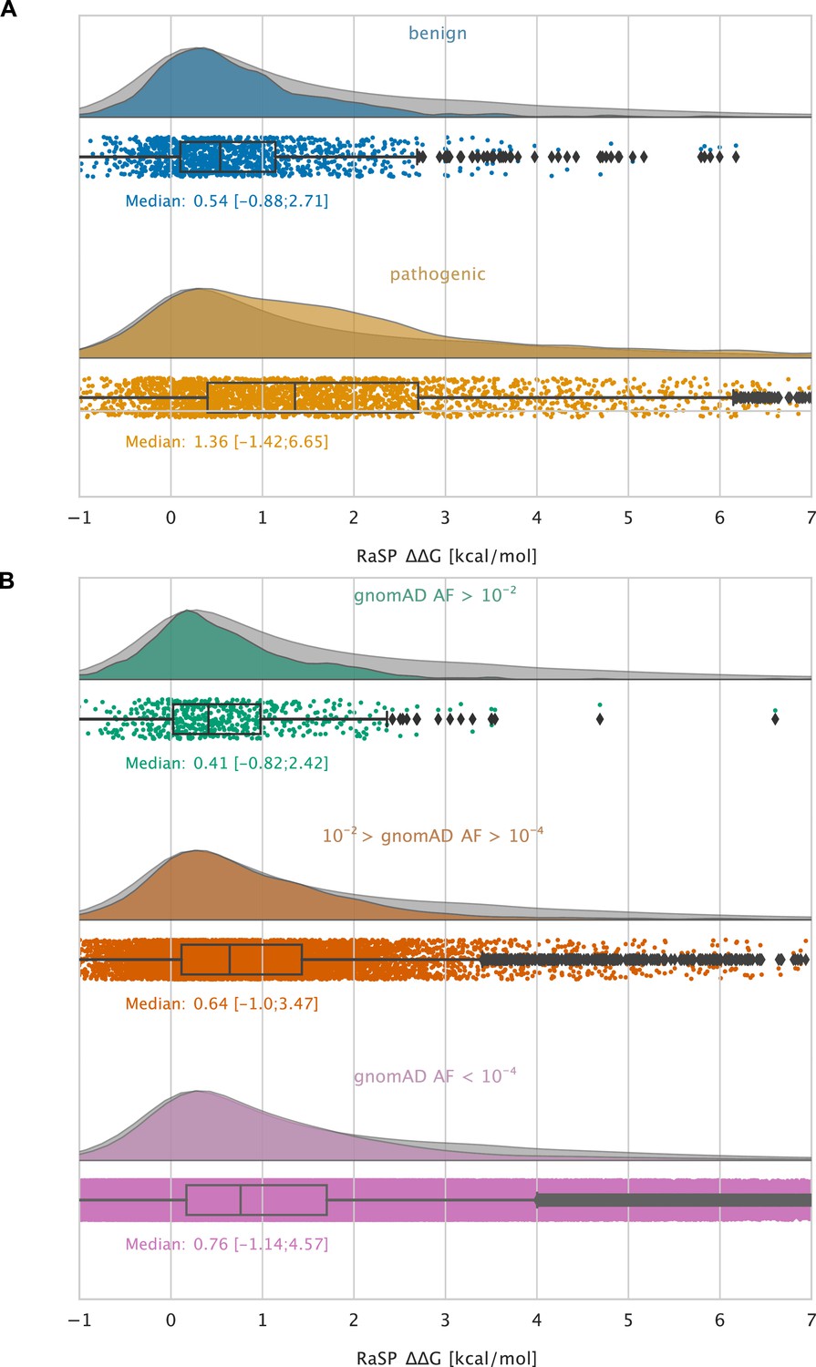
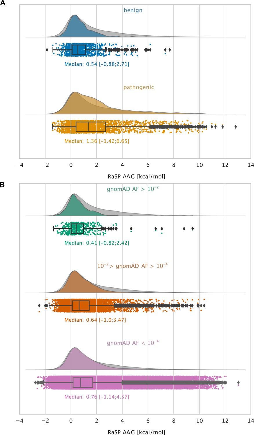
Large-scale analysis of disease-causing variants and variants observed in the population.

The grey distribution shown in the background of all plots represents the distribution of $Δ Δ G$ values calculated using RaSP for all single amino acid changes in the 1,366 proteins that we analysed (15 of the 1381 proteins that we calculated $Δ Δ G$ for did not have variants in ClinVar or gnomAD and were therefore not included in this analysis). Each plot is also labelled with the median $Δ Δ G$ of the subset analysed as well as a range of $Δ Δ G$ values that cover 95% of the data in that subset (box plot shows median, quartiles and outliers). The plots only show values between –1 and 7 kcal/mol (for the full range see Figure 5—figure supplement 2). (A) Distribution of RaSP $Δ Δ G$ values for benign (blue) and pathogenic (tan) variants extracted from the ClinVar database (Landrum et al., 2018). We observe that the median RaSP $Δ Δ G$ value is significantly higher for pathogenic variants compared to benign variants using bootstrapping. (B) Distribution of RaSP $Δ Δ G$ values for variants with different allele frequencies (AF) extracted from the gnomAD database Karczewski et al., 2020 in the ranges (i) AF>10^-2 (green), (ii) 10^-2 > AF>10^-4 (orange), and (iii) AF<10^-4 (purple). We observe a gradual shift in the median RaSP $Δ Δ G$ going from common variants (AF>10^-2) towards rarer ones (AF<10^-4).

Figure 5—figure supplement 1

Download asset Open asset

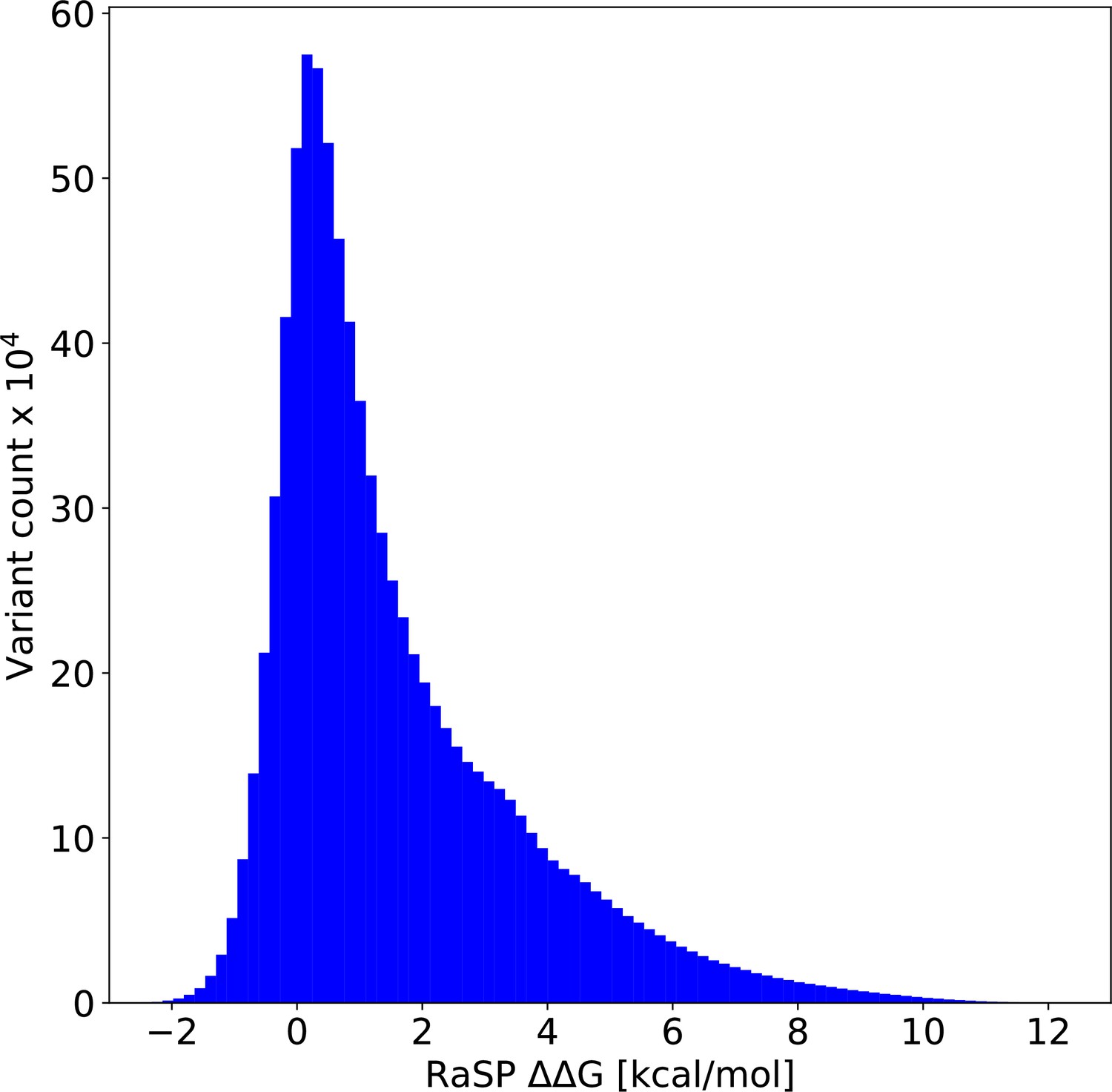
Histogram of $Δ Δ G$ values from saturation mutagenesis using RaSP on 1,366 PDB structures corresponding to ∼8.8 million predicted $Δ Δ G$ values.

Figure 5—figure supplement 2

Download asset Open asset

Large-scale analysis of disease-causing variants and variants observed in the population using the RaSP model.

The grey distribution shown in the background of all plots represents the distribution of $Δ Δ G$ for all single amino acid changes in the 1366 proteins that we analysed. Each plot is also labelled with the median $Δ Δ G$ of the subset analysed as well as a range of $Δ Δ G$ values that cover 95% of the data in that subset (box plot shows median, quartiles and outliers). (A) Distribution of RaSP $Δ Δ G$ values for benign (blue) and pathogenic (tan) variants extracted from the ClinVar database (Landrum et al., 2018). We observe that the median RaSP $Δ Δ G$ value is higher for pathogenic variants compared to benign variants. (B) Distribution of RaSP $Δ Δ G$ values for variants with different allele frequencies (AF) extracted from the gnomAD database Karczewski et al., 2020 in the ranges (i) AF > 10^-2 (green), (ii) 10^-2 > AF > 10^-4 (orange), (iii) AF < 10^-4 (purple). We observe a gradual shift in the median RaSP $Δ Δ G$ going from common variants (AF> 10^-2) towards rarer ones (AF< 10^-4).

Figure 5—figure supplement 3

Download asset Open asset

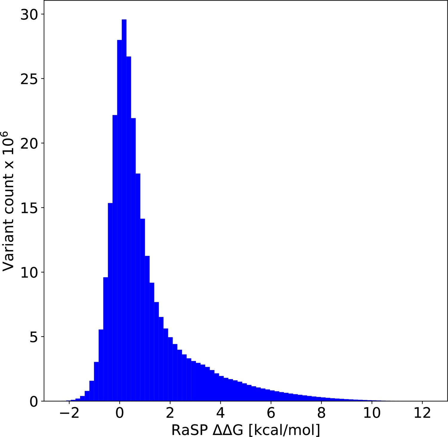
Histogram of $Δ Δ G$ values from saturation mutagenesis using RaSP on predicted structures of the entire human proteome corresponding to ∼300 million predicted $Δ Δ G$ values predicted from 23,391 protein structures.

Tables

Table 1

Overview of RaSP model test set prediction results including benchmark comparison with the Rosetta protocol.

When comparing RaSP to Rosetta (column: "Pearson | $ρ$ | RaSP vs. Ros."), we only compute the Pearson correlation coefficients for variants with a Rosetta $Δ Δ G$ value in the range [–1;7] kcal/mol. Experimental data is from Kumar, 2006; Ó Conchúir et al., 2015; Nisthal et al., 2019; Matreyek et al., 2018; Suiter et al., 2020.

Data set	Protein name	PDB, chain	Pearson \|ρ\| RaSP vs. Ros.	Pearson \|ρ\| RaSP vs. Exp.	Pearson \|ρ\| Ros. vs. Exp.
RaSP test set	MEN1	3U84, A	0.85	-	-
	F8	2R7E, A	0.71	-	-
	ELANE	4WVP, A	0.81	-	-
	ADSL	2J91, A	0.84	-	-
	GCK	4DCH, A	0.84	-	-
	RPE65	4RSC, A	0.84	-	-
	TTR	1F41, A	0.88	-	-
	ELOB	4AJY, B	0.87	-	-
	SOD1	2CJS, A	0.84	-	-
	VANX	1R44, A	0.83	-	-
ProTherm test set	Myoglobin	1BVC, A	0.91	0.71	0.76
	Lysozyme	1LZ1, A	0.80	0.57	0.65
	Chymotrypsin inhib.	2CI2, I	0.79	0.65	0.68
	RNAse H	2RN2, A	0.78	0.79	0.71
Protein G	Protein G	1PGA, A	0.90	0.72	0.72
MAVE test set	NUDT15	5BON, A	0.83	0.50	0.54
	TPMT	2H11, A	0.86	0.48	0.49
	PTEN	1D5R, A	0.87	0.52	0.53

Table 2

Benchmark performance of RaSP versus other structure-based methods on the S669 direct experimental data set (Pancotti et al., 2022).

Results for methods other than RaSP have been copied from Pancotti et al., 2022. We speculate that the higher RMSE and MAE values for Rosetta relative to RaSP are due to missing scaling of Rosetta output onto a scale similar to kcal/mol.

Method	S669, direct
Method	Pearson $ρ$	RMSE [kcal/mol]	MAE [kcal/mol]
Structure-based
ACDC-NN	0.46	1.49	1.05
DDGun3D	0.43	1.60	1.11
PremPS	0.41	1.50	1.08
RaSP	0.39	1.63	1.14
ThermoNet	0.39	1.62	1.17
Rosetta	0.39	2.70	2.08
Dynamut	0.41	1.60	1.19
INPS3D	0.43	1.50	1.07
SDM	0.41	1.67	1.26
PoPMuSiC	0.41	1.51	1.09
MAESTRO	0.50	1.44	1.06
FoldX	0.22	2.30	1.56
DUET	0.41	1.52	1.10
I-Mutant3.0	0.36	1.52	1.12
mCSM	0.36	1.54	1.13
Dynamut2	0.34	1.58	1.15

Table 3

Comparing RaSP predictions from crystal and AlphaFold 2 (AF2) structures.

Pearson correlation coefficients ( $ρ$ ) between RaSP $Δ Δ G$ predictions using either two different crystal structures or a crystal structure and an AlphaFold 2 structure for six test proteins: PRMT5 (X1: 6V0P_A, X2: 4GQB_A), PKM (X1: 6B6U_A, X2: 6NU5_A), FTH1 (X1: 4Y08_A, X2: 4OYN_A), FTL (X1: 5LG8_A, X2: 2FFX_J), PSMA2 (X1: 5LE5_A, X2: 5LE5_O) and GNB1 (X1: 6CRK_B, X2: 5UKL_B). We also divided the analysis into residues with high (pLDDT ≥ 0.9) and medium-low (pLDDT <0.9) pLDDT scores from AlphaFold 2.

Protein	All [ $ρ$ ]			High AF2 pLDDT [ $ρ$ ]			Medium-Low AF2 pLDDT [ $ρ$ ]
Protein	X1-X2	X1-AF2	X2-AF2	X1-X2	X1-AF2	X2-AF2	X1-X2	X1-AF2	X2-AF2
PRMT5	0.93	0.89	0.95	-	0.90	0.95	-	0.66	0.89
PKM	0.99	0.95	0.95	-	0.95	0.95	-	0.88	0.89
FTH1	0.99	0.97	0.97	-	0.97	0.97	-	0.92	0.95
FTL	0.97	0.96	0.97	-	0.96	0.97	-	0.96	0.94
PSMA2	0.99	0.95	0.95	-	0.96	0.96	-	0.78	0.80
GNB1	0.96	0.94	0.94	-	0.94	0.94	-	0.93	0.89

Table 4

Run-time comparison of RaSP and four other methods for three test proteins ELOB (PDB: 4AJY_B, 107 residues), GCK (PBD: 4DCH_A, 434 residues) and F8 (PDB: 2R7E_A, 693 residues).

The RaSP model is in total 480–1,036 times faster than Rosetta. RaSP, ACDC-NN and ThermoNet computations were performed using a single NVIDIA V100 16 GB GPU machine, while Rosetta and FoldX computations were parallelized and run on a server using 64 2.6 GHz AMD Opteron 6380 CPU cores. The number of $Δ Δ G$ computations per mutation was set to 3 for both Rosetta and FoldX. For ThermoNet, we expect that the pre-processing speed can be made comparable to Rosetta via parallelization.

Method	Protein	Wall-clock time [s]
Method	Protein	Pre-processing	$Δ Δ G$	$Δ Δ G$ / residue
RaSP	ELOB	7	41	0.4
	GCK	11	173	0.4
	F8	20	270	0.4
Rosetta	ELOB	677	44,324	414.2
	GCK	7,996	118,361	272.7
	F8	17,211	133,178	192.2
FoldX	ELOB	78	42,237	394.7
	GCK	728	309,762	713.7
	F8	1,306	559,050	806.7
ACDC-NN	ELOB	81	158	1.5
	GCK	169	619	1.4
	F8	325	1,080	1.6
ThermoNet	ELOB	80,442	884	8.3
	GCK	4,586,522	4,227	9.7
	F8	11,627,433	8,732	12.6

Additional files

MDAR checklist: https://cdn.elifesciences.org/articles/82593/elife-82593-mdarchecklist1-v2.docx
Download elife-82593-mdarchecklist1-v2.docx

Download links

A two-part list of links to download the article, or parts of the article, in various formats.

Downloads (link to download the article as PDF)

Open citations (links to open the citations from this article in various online reference manager services)

Mendeley

Cite this article (links to download the citations from this article in formats compatible with various reference manager tools)

Lasse M Blaabjerg
Maher M Kassem
Lydia L Good
Nicolas Jonsson
Matteo Cagiada
Kristoffer E Johansson
Wouter Boomsma
Amelie Stein
Kresten Lindorff-Larsen

(2023)

Rapid protein stability prediction using deep learning representations

eLife 12:e82593.

https://doi.org/10.7554/eLife.82593

Share this article

Cite this article

Overview of model training.

Overview of RaSP downstream model training and testing.

Learning curve for the self-supervised 3D convolutional neural network.

Mean absolute prediction error for RaSP on the validation set, split by amino acid type of the wild-type and variant residue.

RaSP versus Rosetta Δ⁢Δ⁢G values for a full saturation mutagenesis of 10 test proteins separated into either exposed (A) or buried (B) residues.

Comparing RaSP and Rosetta predictions to experimental stability measurements.

Comparing RaSP and Rosetta predictions to experimental stability measurements.

RaSP performance on three recently published data sets (Pancotti et al., 2022): (A) The S669 data set, (B) The Ssym+ direct data set, (C) The Ssym+ reverse data set.

RaSP performance on the recently published mega-scale experiments (Tsuboyama et al., 2022).

Benchmarking RaSP and Rosetta using VAMP-seq data.

Stability predictions from structures created by template-based modelling.

Large-scale analysis of disease-causing variants and variants observed in the population.

Histogram of Δ⁢Δ⁢G values from saturation mutagenesis using RaSP on 1,366 PDB structures corresponding to ∼8.8 million predicted Δ⁢Δ⁢G values.

Large-scale analysis of disease-causing variants and variants observed in the population using the RaSP model.

Histogram of Δ⁢Δ⁢G values from saturation mutagenesis using RaSP on predicted structures of the entire human proteome corresponding to ∼300 million predicted Δ⁢Δ⁢G values predicted from 23,391 protein structures.

Overview of RaSP model test set prediction results including benchmark comparison with the Rosetta protocol.

Benchmark performance of RaSP versus other structure-based methods on the S669 direct experimental data set (Pancotti et al., 2022).

Comparing RaSP predictions from crystal and AlphaFold 2 (AF2) structures.

Run-time comparison of RaSP and four other methods for three test proteins ELOB (PDB: 4AJY_B, 107 residues), GCK (PBD: 4DCH_A, 434 residues) and F8 (PDB: 2R7E_A, 693 residues).

MDAR checklist

Downloads (link to download the article as PDF)

Open citations (links to open the citations from this article in various online reference manager services)

Cite this article (links to download the citations from this article in formats compatible with various reference manager tools)

RaSP versus Rosetta $Δ Δ G$ values for a full saturation mutagenesis of 10 test proteins separated into either exposed (A) or buried (B) residues.

Histogram of $Δ Δ G$ values from saturation mutagenesis using RaSP on 1,366 PDB structures corresponding to ∼8.8 million predicted $Δ Δ G$ values.

Histogram of $Δ Δ G$ values from saturation mutagenesis using RaSP on predicted structures of the entire human proteome corresponding to ∼300 million predicted $Δ Δ G$ values predicted from 23,391 protein structures.