Polygenic adaptation from standing genetic variation allows rapid ecotype formation
Figures
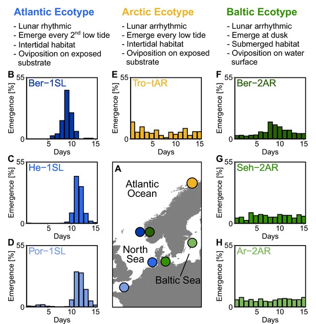
Northern European ecotypes of Clunio and their circalunar rhythms.
The Atlantic, Arctic and Baltic ecotypes of Clunio differ mainly in their circalunar rhythms (B–H), circadian rhythms (Figure 1—figure supplement 1), as well as their habitat and the resulting oviposition behavior (see ‘Assessment of oviposition behavior’ in Methods section). (A) Sampling sites for this study. (B–H) Circalunar rhythms of adult emergence in corresponding laboratory strains under common garden conditions, with 16 hours of daylight and simulated tidal turbulence cycles to synchronize the lunar rhythm. In Arctic and Baltic ecotypes the lunar rhythm is absent (E,G,H) or very weak (F). Por-1SL: n=1,263; He-1SL: n=2,075; Ber-1SL: n=230; Tro-tAR: n=209; Ber-2AR: n=399; Seh-2AR: n=380; Ar-2AR: n=765.
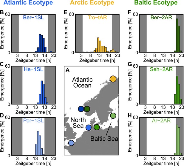
Circadian emergence rhythm of the studied Clunio strains under laboratory conditions.
(A) Geographic locations. (B–H) Circadian emergence rhythms of laboratory strains. Dark shading indicates the dark phase, the middle of dark phase is defined as zeitgeber time 0. Data for Ber-1SL (B; n=130), Ber-2AR (F; n=36) and Tro-tAR (E; n=99) was recorded with a custom-made fraction collector in 1 h intervals under an artificial light cycle with 16 hr of light and 8 hr of darkness (LD 16:8). Data for Seh-2AR (G; n=70) and Ar-2AR (H; n=25) was recorded manually while performing crosses. Data of He-1SL (C) and Por-1SL (D) was taken from Neumann, 1966 and recorded under LD 12:12.
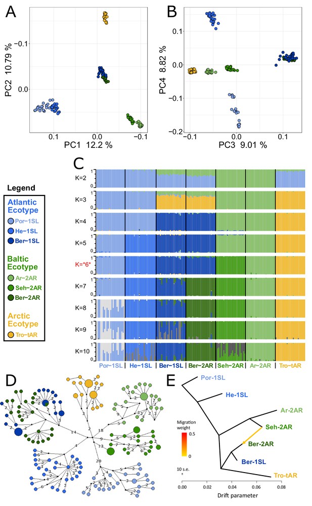
Genetic structure and evolutionary history of Northern European Clunio ecotypes.
The analysis is based on 24 individuals from each population (23 for Por-1SL, 25 for He-1SL). (A, B) Principal Component Analysis (PCA) based on 792,032 SNPs separates populations by geographic location rather than ecotype. (C) ADMIXTURE analysis supports strong differentiation by geographic site (best K=6), but a notable genetic component from the Baltic Sea in the Bergen populations (see K=2 and 3). The Bergen populations are only separated at K=7 and then show a number of admixed individuals. (D) Haplotype network of full mitochondrial genomes reveals highly divergent clusters according to geographic site, but haplotype sharing between Ber-1SL and Ber-2AR. (E) Correlated allele frequencies indicate introgression from Seh-2AR into Ber-2AR.
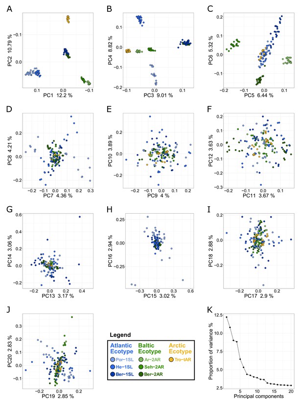
Principal component analysis (PCA) of all individuals for all seven populations.
(A–J) The principal components (PCs) are plotted in pairs from 1-2 (A) to 19–20 (J). The eigenvalue as fraction of total variance is given on the respective axes. The individuals are color-coded according to population (see legend). (K) Overview of the eigenvalue as fraction of total variance for all 20 PCs.
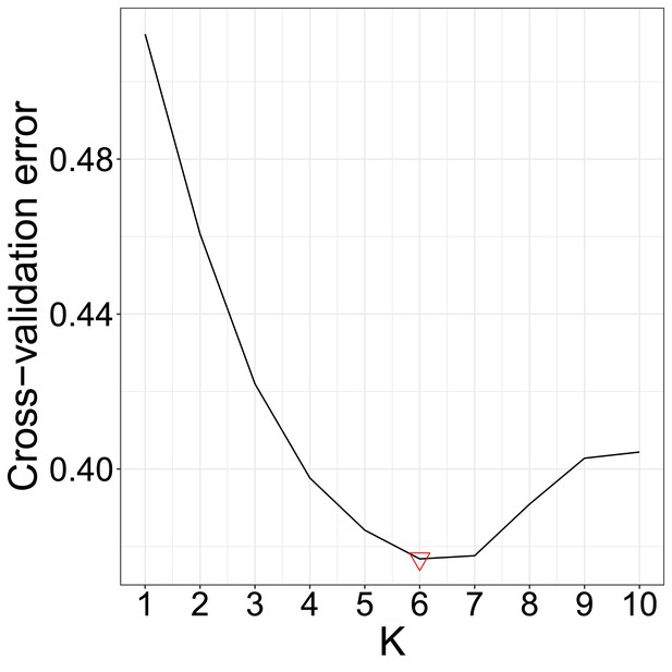
The results of the cross-validation test of the ADMIXTURE analysis.
The optimal K is marked with a red downward directed triangle.
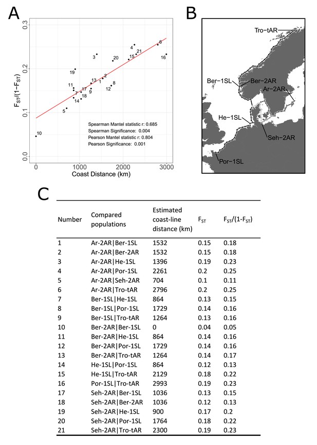
Mantel test for isolation by distance between the studied populations.
(A) The average genomic differentiation is plotted against the estimated coastline distance on a pairwise level. Results of the Spearman and Pearson Mantel statistic are noted in the lower right corner of the graph. A trendline is drawn in red. (B) The coastline distance was measured on a map in 50 km intervals. Distances between certain locations had different shortest distances, which are colored in different gray tones. (C) Every pairwise comparison is listed by number, the population names, the estimated coastline distance in km, their average FST value and the FST/(1-FST) values.
-
Figure 2—figure supplement 3—source data 1
Table of the input data for the Mantel test.
- https://cdn.elifesciences.org/articles/82824/elife-82824-fig2-figsupp3-data1-v3.xlsx
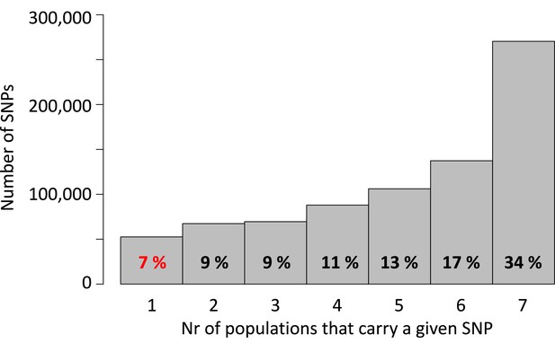
Detected single nucleotide polymorphisms (SNPs) are largely shared between the seven populations.
Of a total of 792,032 SNPs, 34% are found in all seven populations, whereas only 7% are private to one of the seven populations.
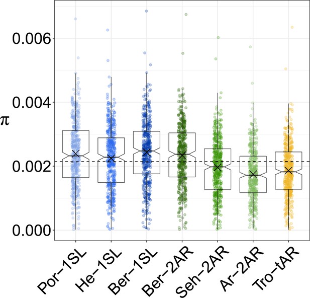
Nucleotide diversity π per population in 200 kb non-overlapping windows across the genome.
Populations are color-coded as in Figure 1A and all individuals per population were used for the analysis. The boxplots show the median, 25th and 75th quantile, data maximum and minimum, and the outliers. The arithmetic mean is marked per boxplot as 'X' and the overall arithmetic mean as dashed line. Statistical tests are given in Supplementary file 1.
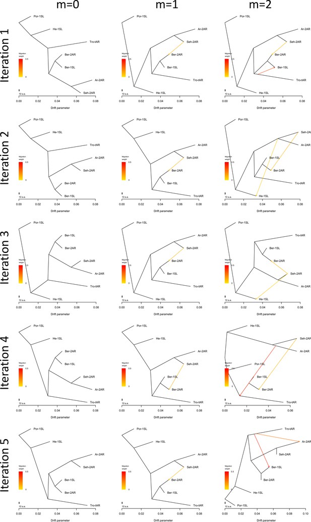
TreeMix analysis for introgression events.
TreeMix was run for no, one or two migration events with five iterations each. Analysis with zero migration events yields the same structure of historic population splits in all five iterations, congruent with the genome-wide consensus phylogeny (Figure 3—figure supplement 2). With one migration event, the algorithm stably detects introgression from Seh-2AR into Ber-2AR. With two migration events, introgression from Seh-2AR into Ber-2AR is usually still detected (4 out of 5 iterations), but the second introgression event is random, suggesting there is no reliably detectable second introgression event.
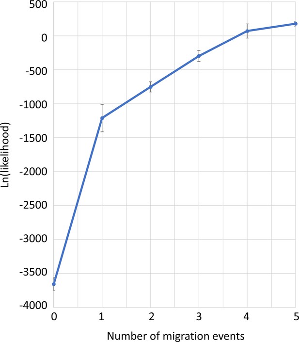
Model likelihood in TreeMix analysis, dependent on the number of assumed migration events.
The mean and standard deviation for 8 runs is given. The flattening of the line at after one migration event suggests that one migration event is the best assumption. This is congruent with the fact that starting from two migration events the iterations get incongruent with respect to the source, target, and direction of migration.
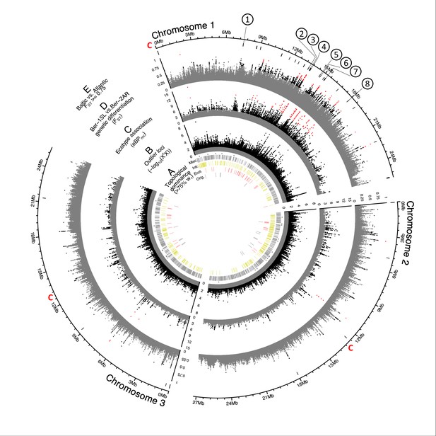
Genome screens for haplotype sharing and genotype-ecotype associations.
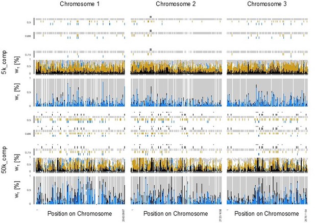
(A) Topology weighting of phylogenetic trees for 36 individuals from the Baltic and Atlantic ecotypes, as obtained from 50 kb non-overlapping genomic windows. Windows were marked by a bar if they were dominated by one kind of topology (wτ>75%). Most windows are not dominated by the consensus population topology (‘Orig.’; Figure 3—figure supplement 2), but by combinations of other topologies (‘Misc.’). Windows dominated by topologies that separate the Baltic and Atlantic ecotypes (‘Ecol.’) are mostly on chromosome 1. Windows consistent with introgression are found all over the genome (‘Intr.’). (B) Distribution of outlier variants (SNPs and Indels) between the six Baltic and Atlantic ecotype populations, after global correction for population structure (XtX statistic). Values below the significance threshold (as obtained by subsampling) are plotted in gray. (C) Association of variant frequencies with Baltic vs. Atlantic ecotype (eBPmc). Values below the threshold of 3 (corresponding to p=10–3) are given in gray, values above 10 are given in red. (D) Genetic differentiation (FST) between the sympatric ecotypes in Bergen. Values above 0.5 are given in black, values above 0.75 in red. (E) The distribution of SNPs with FST ≥ 0.75 in the Baltic vs. Atlantic ecotypes. Circled numbers mark the location of the eight most differentiated loci (see Figure 6). Centromeres of the chromosomes are marked by a red ‘C’.
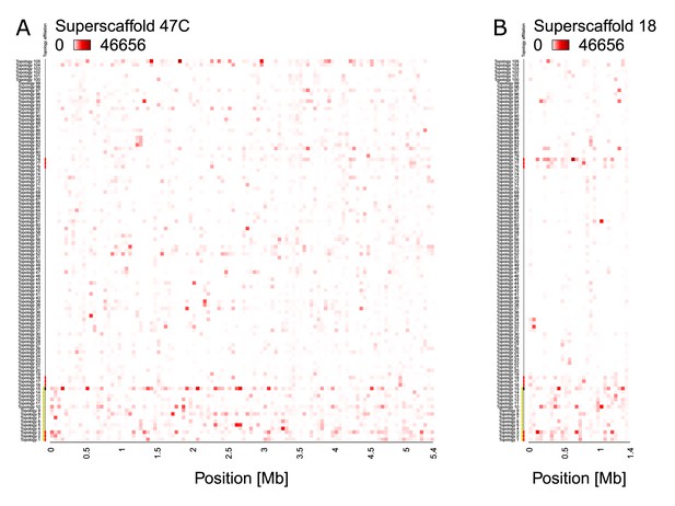
Incomplete lineage sorting, as illustrated by the relative support for 105 population topologies in 50 kb windows across superscaffolds 47 C and 18.
The heatmap shows the assigned topology weight for each topology per window ranging from 0 (white, no support) to 46,656 (red, support by all trees). The supported topologies change quickly along the chromosome. In almost all windows, several topologies are supported, which implies that individuals do not cluster according to population, highlighting incomplete lineage sorting. Topology 15 (black mark on the left) is the whole-genome consensus population topology. Topologies marked in red are separating populations according to ecotypes. Topologies marked in yellow are consistent with introgression. (A) Superscaffold47C – the longest scaffold in the reference genome – gives an impression of the genomic background, with highest overall support for topology 15. (B) Superscaffold 18, from the middle of chromosome 1, is strongly enriched for ecotype-associated topologies (compare Figure 3).
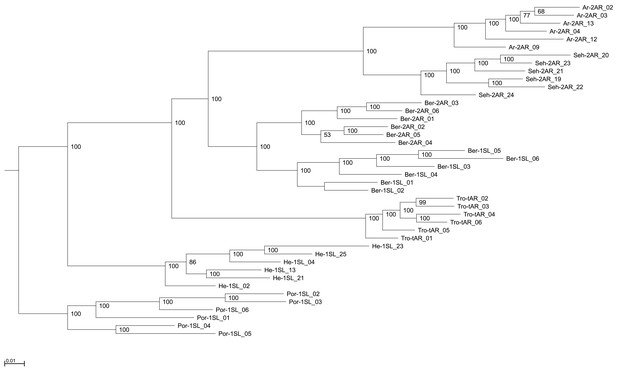
Genome-wide consensus genealogy for six individuals from each of the seven populations.
The same six individuals from each population were also used in the TWISST topology weighting analysis. The genealogy is based on the whole genome SNP sequences, composed of 792,032 positions. The SNPs were extracted from the VCF using the vcf2phylip.py v.2.3 script. The genealogy was calculated with IQ-TREE v.1.6.12 and graphically edited with Archaeopteryx v.0.968.
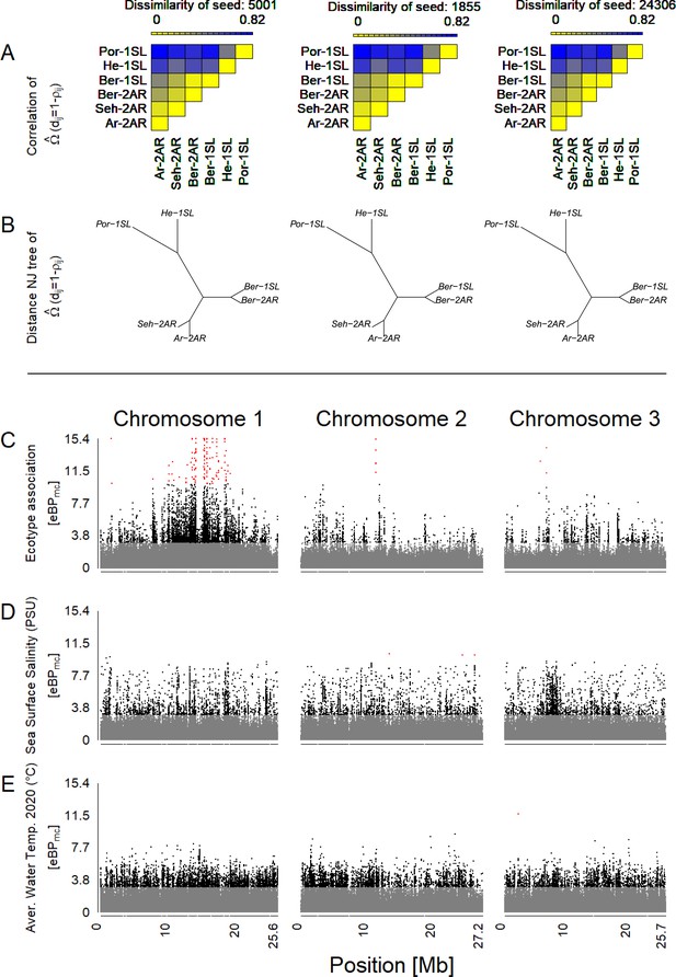
An overview of outlier and association analysis for ecotype (C), sea surface salinity (D) and water temperature (E).
(A) Before assessment of outlier loci and association, the dataset was corrected for population structure based on an Omega matrix, which is here visualized as a dissimilarity matrix. Three independent runs (seeds 5001, 1855, and 24,306) converge. (B) Omega matrices can also be visualized as Neighbour Joining trees. (C–E) Association of genetic variants with ecotype (C), sea surface salinity (D) and water temperature (E) is assessed via the eBPmc score and plotted along the three chromosomes, color-coded in gray (eBPmc <3), black (3<eBPmc < 10), and red (eBPmc >10).
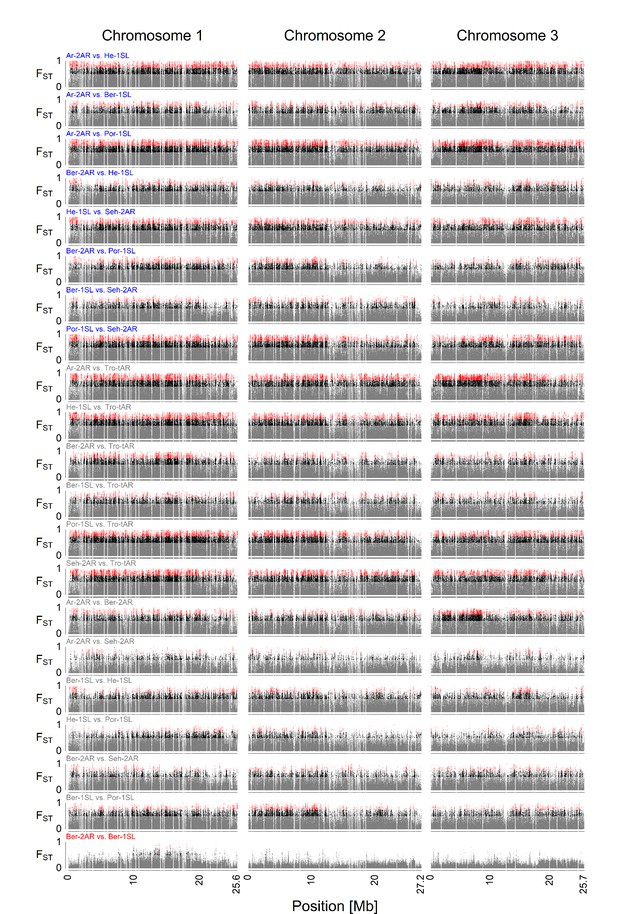
Pairwise FST comparisons between all seven populations.
The specific populations of the comparison are written above each plot, color-coded for specific comparisons. The comparison between the sympatric Ber-2AR and Ber-1SL ecotypes is plotted in red. Other comparisons of Atlantic vs. Baltic ecotype populations are plotted in blue. All other comparisons are plotted in gray. The FST values are color-coded in gaey (FST <0.5), black (0.5<FST < 0.75), and red (FST >0.75). The sympatric ecotypes from Bergen are much less differentiated than all other populations.
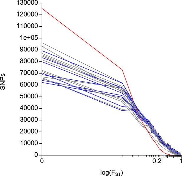
Distribution of FST values in all pairwise population comparisons.
FST values for 792,032 SNPs were categorized in 0.02 bins. The comparison between the sympatric Ber-2AR and Ber-1SL ecotypes is plotted in red. Other comparisons of Atlantic vs. Baltic ecotype populations are plotted in blue. All other comparisons are plotted in gray.

Genetic differentiation (FST) between Atlantic and Baltic ecotype.
Atlantic ecotype populations (Por-1SL, He-1SL, Ber-1SL) and Baltic ecotype populations (Ar-2AR, Seh-2AR, Ber-2AR) were grouped. The FST values are color-coded in gray (FST<0.5), black (0.5<FST< 0.75), and red (FST>0.75).
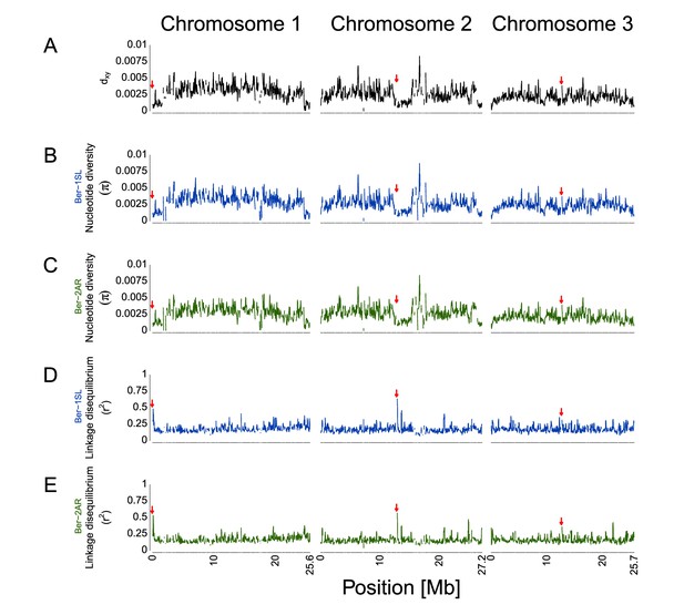
Genetic divergence (dxy), nucleotide diversity (π) and short-range linkage disequilibrium (r2) for the Ber-2AR vs. Ber-1SL comparison.
Summary statistics are based on 792,032 SNPs and were calculated in 100 kb sliding windows with 10 kb steps. (A) Genetic divergence (dxy) based on allele frequencies. (B, C) Nucleotide diversity π. (D, E) Linkage disequilibrium measured as r2. Ber-1SL and Ber-2AR are given in their respective population colors. The approximate position of the centromeres are marked on each chromosome with red arrows. The position is based on the data provided by Kaiser et al., 2016.
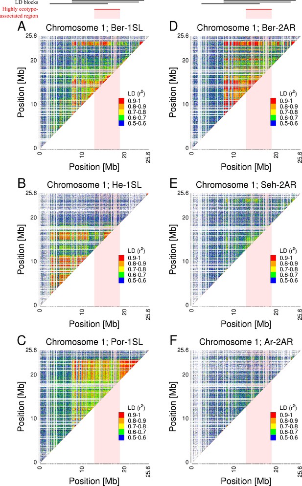
Pairwise linkage disequilibrium (LD) across chromosome 1 of all Atlantic and Baltic ecotype populations.
Pairwise LD was calculated as ‘--geno-r2’ in VCFtools with a ‘--maf 0.2’ filter and a LD threshold of 0.5 r2. The r2 values are color-coded from 0.5 (blue) to 1 (red) in 0.1 steps. The panels show the chromosome 1 r2 values for each population (A: Ber-1SL, B: He-1SL, C: Por-1SL, D: Ber-2AR, E: Seh-2AR, F: Ar-2AR).
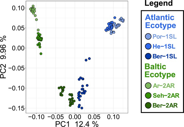
Principal component analysis (PCA) of the Atlantic and Baltic ecotypes for the highly ecotype-assocated region on chromosome 1.
The highly ecotype-associated region on chromosome 1 ranges from superscaffolds 18–42. PCA for this region separates the ecotypes well, but does not show any patterns characteristic for a polymorphic structural variant (SV) separating the ecotypes. Only within the Por-1SL strain individuals cluster into three groups, suggestive of an overlapping polymorphic SV within that strain.
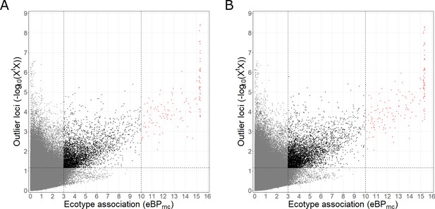
Selection of ecotype associated genetic variants based on XtX and eBPmc values.
(A) Ecotype-associated SNPs were selected based on an XtX threshold of 1.152094 (as obtained from subsampling) and eBPmc thresholds of 3 or 10 respectively (corresponding to p-values for association of 10–3 or 10–10). SNPs above the XtX threshold and with eBPmc >3 are colored black, those with eBPmc >10 are colored in red. (B) Ecotype-associated variants (SNPs and indels) were selected based on an XtX threshold of 1.148764 and the same eBPmc thresholds.
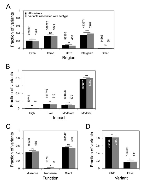
The effects of ecotype-associated genetic variants on genes, as compared to the genome-wide set of genetic variants.
SnpEff assesses genetic variants for their position relative to annotated gene models and infers the effect that these variants have on the genes. We compared the locations and effects of all variants in the dataset (n=948,128; black bars) to those of ecotype-associated variants (n=4,741; gray bars) and tested for significant differences with Fisher’s exact test. The absolute numbers for each class of variants are given above or inside the bar. (A) The location of genetic variants relative to gene models. (B) The estimated impact of these variants on the gene models. (C) The effect of variants that are found in coding regions. (D) The proportions of SNPs vs. indels. p-value symbols: **** - 0–0.0001; *** - 0.0001–0.001; ** - 0.001–0.01; * - 0.01–0.05; ns - 0.05–1.

Linkage disequilibrium (LD) decay in the studied C.marinus populations.
Populations were analyzed separately and the corresponding lines in each plot are color-coded. To make a pairwise LD calculation measured as r2 feasible, the SNP set was randomly subsampled to 25%. The distance between the SNPs was limited to 500 bp for LD calculation. The resulting r2 values were then averaged within 30 average-distance-classes.
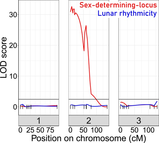
Quantitative Trait Locus (QTL) mapping for lunar rhythmicity (blue) and the sex determining locus (red).
The sex-determining locus is clearly detectable (red). No significant QTLs can be detected for lunar rhythmicity, suggesting it is controlled by more than one locus. Vertical black lines are genetic markers.
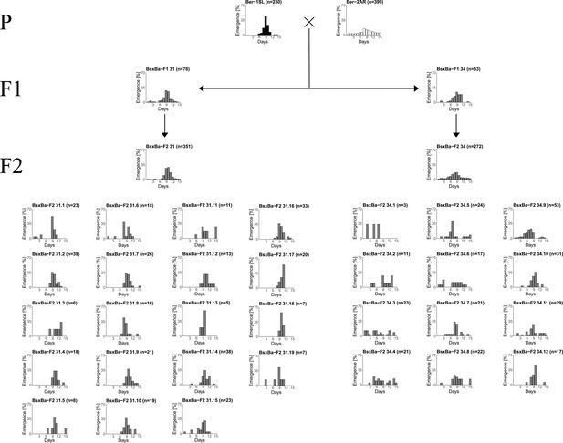
Lunar emergence patterns of crosses between the Ber-1SL and Ber-2AR strains.
Single pair crosses were set up between the Ber-1SL and Ber-2AR strains, resulting in several F1 families, two of which are shown here (BsxBa-F1-31 and BsxBa-F1-34). F2 families were obtained by letting the siblings within each F1 family mate freely with each other. Thus, from each F1 we obtained several F2 families, which all go back to a single pair of parents. F1-31 and F1-34 differ in the degree of lunar rhythmicity, as do F2-31 and F2-34. When plotting the F2 families individually, it becomes apparent that in F2-31 all families are quite rhythmic. In contrast, in F2-34 there are highly rhythmic families (e.g. F2-34.10) and completely arrhythmic families (e.g. F2-34.3 and F2-34.4), suggesting that this F2 generation is segregating for rhythmicity alleles. The observation suggests that in the cross leading to F1-31/F2-31, the Ber-2AR parent carried a considerable fraction of rhythmic alleles (basically ‘Ber-1SL’ alleles), which rendered the resulting F1 and F2 generations largely rhythmic. The Ber-2AR parent for the F1-34/F2-34 cross seemed to carry largely arrhythmic alleles, as expected, which then segregate in the F2. Overall, we conclude that the Ber-2AR strain seems to carry a certain fraction of lunar rhythmic alleles. The segregation of lunar rhythmicity not only within but also between F2 families suggests a heterogeneous polygenic architecture of the trait.

Genetic and physical location of the designed genetic markers across the genome of Clunio.
The upper part of the figure shows marker names and their positions on the genetic map (continuous gray bars). The genetic position in centimorgan is noted after the marker name. The Manhattan plot shows the genetic differentiation (FST) between the populations Ber-2AR and Ber-1SL on the physical map. The scaffolds of the genome chromosomes are subdivided by colors to indicate approximately equally sized regions on the physical map. The FST values are color-coded in gray (FST <0.5), black (0.5 ≤ FST < 0.75), and red (FST ≤ 0.75). The position of the markers are linked between the genetic and the physical map with black lines.
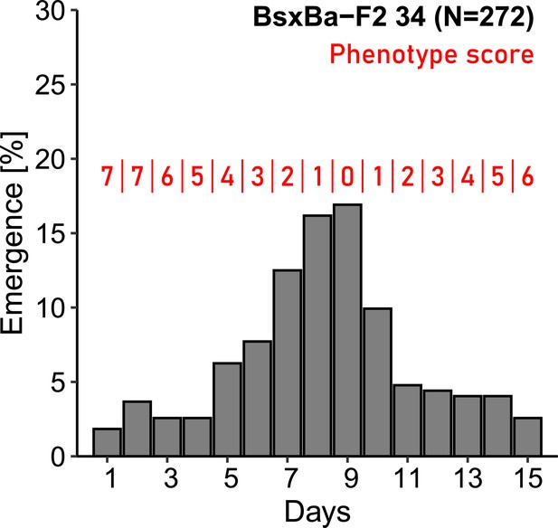
Phenotyping of the F2 individuals based on their emergence day.
Lunar rhythmicity in the individuals was scored based on their emergence day, in relation to the Ber-1SL emergence distribution peak on day 9 of the 15-day turbulence cycle.
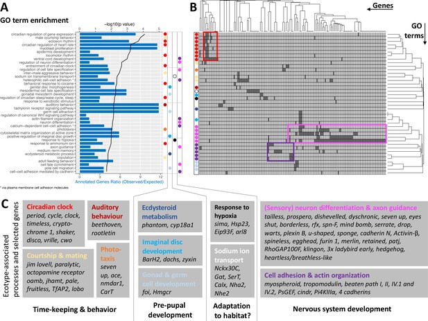
GO term analysis of ecotype associated SNPs (A) The top 40 enriched GO terms are listed for the 1,400 genes that are found to be affected by ecotype-associated genetic variants (eBPmc >3).
For each GO term, the significance level (black line, top y-axis) and the observed-expected ratio of genes annotated to the respective GO term (blue bars, bottom y-axis) are given. (B) The top 40 GO terms are driven by 168 genes. Hierarchical clustering of genes and GO terms reveals major signals in the circadian clock and nervous system development (more details in Supplementary file 8). (C) Most GO terms are consistent with the known ecotype differences and selected genes are highlighted for all of them. Notably, basically all core circadian clock genes are affected.
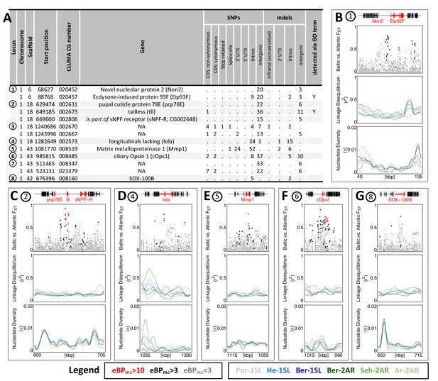
The 13 most differentiated ecotype-associated genes (A) Loci with highly ecotype-associated variants were selected based on eBPmc >10 and FST(Baltic-Atlantic)>0.75.
There are 13 genes in eight distinct genomic loci. (B–G) An overview is given for the six loci with identified genes. In each panel, from top to bottom the sub-panels show the gene models, FST values of genetic variants in the region, local linkage disequilibrium (LD) and genetic diversity (). FST values are colored by ecotype association of the variant (red: eBPmc >10; black: 10>eBPmc > 3; gray: eBPmc <3). LD and genetic diversity are shown for the six populations independently, colored-coded as in Figures 1 and 2 (10 kb overlapping sliding-windows with 1 kb steps). The are no strong signatures of selection.
-
Figure 6—source data 1
Table of loci with highly ecotype-associated variants.
- https://cdn.elifesciences.org/articles/82824/elife-82824-fig6-data1-v3.xlsx
Additional files
-
Supplementary file 1
Wilcoxon rank sum test with continuity correction for significant differences in nucleotide diversity (π) between populations, based on the arithmetic mean of 200 kb genomic windows.
The lower-left part of the table shows the p-values and the upper-right part the corresponding significance levels: **** - 0–0.0001; *** - 0.0001–0.001; ** - 0.001–0.01; * - 0.01–0.05; ns - 0.05–1.
- https://cdn.elifesciences.org/articles/82824/elife-82824-supp1-v3.xlsx
-
Supplementary file 2
Twisst output.
- https://cdn.elifesciences.org/articles/82824/elife-82824-supp2-v3.zip
-
Supplementary file 3
Filtered gene annotations for the CLUMA1.0 genome assembly.
- https://cdn.elifesciences.org/articles/82824/elife-82824-supp3-v3.zip
-
Supplementary file 4
SnpEff analysis for selected and all variants.
SnpEff was run on the selected BayPass ecotype-associated variants and on all variants. For each analytical group (Region, Impact, Function, Variant) the total numbers for each subgroup and the fractions in respect to the entire analytical group are given. Additionally, the p-values for significant deviation between the selected and entire genome variants were calculated using Fisher’s exact test.
- https://cdn.elifesciences.org/articles/82824/elife-82824-supp4-v3.xlsx
-
Supplementary file 5
Genes with eBPmc larger than 3.
- https://cdn.elifesciences.org/articles/82824/elife-82824-supp5-v3.xlsx
-
Supplementary file 6
SNPeff results for genes with eBPmc larger than 3.
- https://cdn.elifesciences.org/articles/82824/elife-82824-supp6-v3.zip
-
Supplementary file 7
GO term annotations for the CLUMA1.0 genome assembly.
- https://cdn.elifesciences.org/articles/82824/elife-82824-supp7-v3.txt
-
Supplementary file 8
List of genes with ecotype-associated variants, which drive the top 40 GO terms in GOterm enrichment analysis.
Gene identity was individually confirmed (see column "Gene_Name_curated"). The order of genes and GO terms corresponds to Figure 4B.
- https://cdn.elifesciences.org/articles/82824/elife-82824-supp8-v3.xlsx
-
Supplementary file 9
Genes with eBPmc larger than 10.
- https://cdn.elifesciences.org/articles/82824/elife-82824-supp9-v3.xlsx
-
Supplementary file 10
SNPeff results for genes with eBPmc larger than 10.
- https://cdn.elifesciences.org/articles/82824/elife-82824-supp10-v3.zip
-
Supplementary file 11
Sampling sites and sampling campaigns for the five newly established laboratory strains in this study.
On sampling dates in squared brackets egg clutches for setting up laboratory cultures were collected from copulating pairs on the water surface. Samples from underlined dates were used for the genomic analyses of the wild populations.
- https://cdn.elifesciences.org/articles/82824/elife-82824-supp11-v3.xlsx
-
Supplementary file 12
Multiplex PCR primer pairs for QTL mapping between the sympatric populations Ber-1SL and Ber-2AR.
All primers were designed and tested by Kerstin Schaefer.
- https://cdn.elifesciences.org/articles/82824/elife-82824-supp12-v3.xlsx
-
Supplementary file 13
Volume modifications for the REPLI-g Mini Kit QIAGEN 150025 whole genome amplification kit (QIAGEN).
MM – Master Mix.
- https://cdn.elifesciences.org/articles/82824/elife-82824-supp13-v3.xlsx
-
Supplementary file 14
The three covariates used for association analysis in BayPass.
- https://cdn.elifesciences.org/articles/82824/elife-82824-supp14-v3.xlsx
-
MDAR checklist
- https://cdn.elifesciences.org/articles/82824/elife-82824-mdarchecklist1-v3.docx


