Polygenic adaptation from standing genetic variation allows rapid ecotype formation

Abstract
Editor's evaluation
Introduction
Results
Discussion
Methods
Data availability
References
Article and author information
Metrics

Abstract

Adaptive ecotype formation can be the first step to speciation, but the genetic underpinnings of this process are poorly understood. Marine midges of the genus Clunio (Diptera) have recolonized Northern European shore areas after the last glaciation. In response to local tide conditions they have formed different ecotypes with respect to timing of adult emergence, oviposition behavior and larval habitat. Genomic analysis confirms the recent establishment of these ecotypes, reflected in massive haplotype sharing between ecotypes, irrespective of whether there is ongoing gene flow or geographic isolation. QTL mapping and genome screens reveal patterns of polygenic adaptation from standing genetic variation. Ecotype-associated loci prominently include circadian clock genes, as well as genes affecting sensory perception and nervous system development, hinting to a central role of these processes in ecotype formation. Our data show that adaptive ecotype formation can occur rapidly, with ongoing gene flow and largely based on a re-assortment of existing alleles.

Editor's evaluation

This valuable study combines phenotypic analysis, quantitative genetics and population genomics to provide solid evidence for multiple genes underlying adaptive divergence in a marine midge system linked to tidal rhythm. Genes with a plausible role in perceiving and responding to lunar information are among the loci that most highly differentiate populations with distinct behaviors.

https://doi.org/10.7554/eLife.82824.sa0

Introduction

The genetic foundations for rapid ecological adaptation and speciation remain poorly understood. Decades of research have focused on identifying single or few major genetic loci in such contexts, with some notable successes (Wu and Ting, 2004; Phadnis and Orr, 2009; Nosil and Schluter, 2011; Van’t Hof et al., 2016). However, many genome-wide association studies have now shown that quantitative trait phenotypes have usually a polygenic basis (Sella and Barton, 2019; Boyle et al., 2017). This implies that also rapid natural adaptation should be expected to occur in a polygenic context, based on subtle allele frequency changes at many loci with small effects (Barton, 2022; Barghi et al., 2020; Le Corre and Kremer, 2012). A classic example for polygenic adaptation is human height (Turchin et al., 2012; Robinson et al., 2015), and other examples from humans may include birth weight and female hip size (Field et al., 2016). However, powerful datasets to detect polygenic adaptations are still mostly limited to humans and agriculturally relevant species (Barghi et al., 2020), and examples of polygenic adaptation in natural populations are rare. To show that polygenic adaptation occurs in natural populations requires an exceptional biogeographic setting, as well as deep genomic and genetic analysis. One such example may be found in Midas cichlids, where a polygenic trait architecture was found to promote rapid and stable sympatric speciation (Kautt et al., 2020). This finding is particularly interesting, since theoretical work suggested that under scenarios with gene flow the genetic architecture of adaptation may – compared to adaptation without gene flow – rather consist of fewer, tightly linked loci with larger effects (Yeaman and Whitlock, 2011). Notably, the same study also suggested that the resulting large-effect QTL may often be composed of many tightly linked loci of smaller effects (Yeaman and Whitlock, 2011). Without migration we expect an exponential distribution of allele effects, with few large effect loci and many loci of small effects (Barghi et al., 2020; Orr, 1998).

In this study, we examine local adaptation and population divergence in another exceptional biogeographic setting, namely the postglacial evolution of new ecotypes in marine midges of the genus Clunio (Diptera: Chironomidae). In adaptation to their habitat, Clunio midges differ in oviposition behavior and reproductive timing, involving both circadian and circalunar clocks.

Circalunar clocks are biological time-keeping mechanisms that allow organisms to anticipate lunar phase (Neumann, 2014). Their molecular basis is unknown (Andreatta and Tessmar-Raible, 2020), making identification of adaptive loci for lunar timing both particularly challenging and interesting. In many marine organisms, circalunar clocks synchronize reproduction within a population. In Clunio marinus they have additional ecological relevance (Kaiser, 2014). Living in the intertidal zone of the European Atlantic coasts, C. marinus requires the habitat to be exposed by the tide for successful oviposition. The habitat is maximally exposed during the low waters of spring tide days around full moon and new moon. Adult emergence is restricted to these occasions by a circalunar clock, which tightly regulates development and maturation. Additionally, a circadian clock ensures emergence during only one of the two daily low tides. The adults reproduce immediately after emergence and die few hours later. As tidal regimes vary dramatically along the coastline, populations of this Atlantic ecotype of C. marinus show local timing adaptations (Kaiser, 2014; Neumann, 1967; Kaiser et al., 2011) for which the genetic underpinnings are partially known (Kaiser et al., 2016; Kaiser and Heckel, 2012).

When Clunio expanded into the North after the regression of the ice shield, new ecotypes evolved in the Baltic Sea (Remmert, 1955; Palmén and Lindeberg, 1959) and in the high Arctic (Neumann and Honegger, 1969; Pflüger and Neumann, 1971), which differ from the Atlantic ecotype of C. marinus in various ways (see Figure 1 for a summary of defining characteristics of the three ecotypes). In the Baltic Sea the tides are negligible and the Baltic ecotype oviposits on the open water, from where the eggs quickly sink to the submerged larval habitat at water depths of up to 20 m (Remmert, 1955; Endraß, 1976a). Reproduction of the Baltic ecotype happens every day precisely at dusk under control of a circadian clock (Heimbach, 1978), without a detectable circalunar rhythm (Endraß, 1976a). Near Bergen (Norway) the Baltic and Atlantic ecotypes were reported to co-occur in sympatry, but in temporal reproductive isolation. The Baltic ecotype reproduces at dusk, the Atlantic ecotype reproduces during the afternoon low tide (Heimbach, 1978). Therefore, the Baltic ecotype is currently considered a separate species – C. balticus. However, C. balticus and C. marinus can be successfully interbred in the laboratory (Heimbach, 1978).

Figure 1 with 1 supplement see all

Download asset Open asset

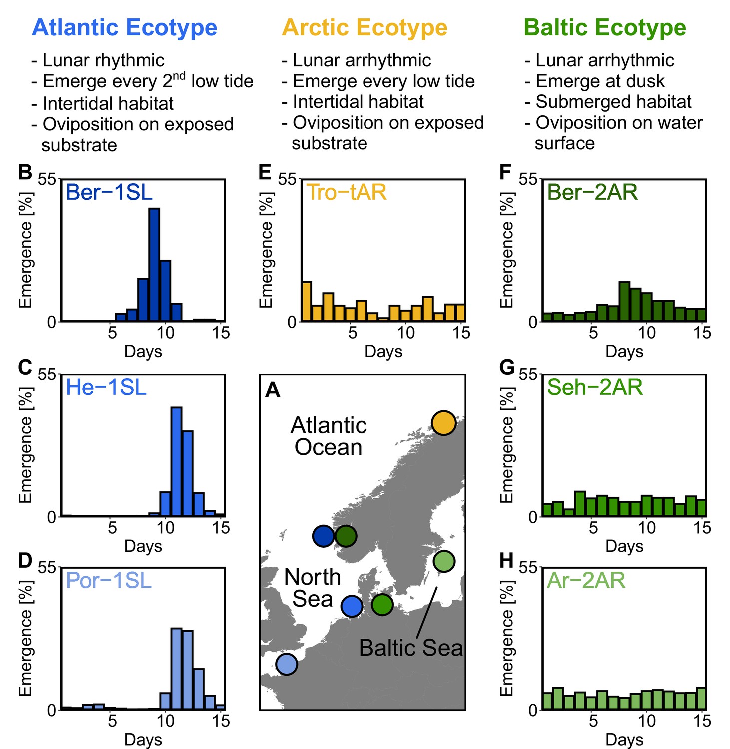
Northern European ecotypes of *Clunio* and their circalunar rhythms.

The *Atlantic*, *Arctic* and *Baltic ecotypes* of *Clunio* differ mainly in their circalunar rhythms (**B–H**), circadian rhythms (Figure 1—figure supplement 1), as well as their habitat and the resulting oviposition behavior (see ‘Assessment of oviposition behavior’ in Methods section). (A) Sampling sites for this study. (**B–H**) Circalunar rhythms of adult emergence in corresponding laboratory strains under common garden conditions, with 16 hours of daylight and simulated tidal turbulence cycles to synchronize the lunar rhythm. In *Arctic* and *Baltic ecotypes* the lunar rhythm is absent (**E,G,H**) or very weak (F). Por-1SL: n=1,263; He-1SL: n=2,075; Ber-1SL: n=230; Tro-tAR: n=209; Ber-2AR: n=399; Seh-2AR: n=380; Ar-2AR: n=765.

In the high Arctic there are normal tides and the Arctic ecotype of C. marinus is found in intertidal habitats (Neumann and Honegger, 1969). During its reproductive season, the permanent light of polar day precludes synchronization of the circadian and circalunar clocks with the environment. Thus, the Arctic ecotype relies on a so-called tidal hourglass timer, which allows it to emerge and reproduce during every low tide (Pflüger and Neumann, 1971). It does not show circalunar or circadian rhythms (Pflüger and Neumann, 1971).

The geological history of Northern Europe (Patton et al., 2017) implies the Baltic Sea and the high Arctic could only be colonized by Clunio after the last glacial ice shield regressed about 10,000 years ago. This inference is also supported by subfossil Clunio head capsules in Baltic Sea sediment cores (Hofmann and Winn, 2000). The new adaptations to the absence of tides in the Baltic Sea and to polar day in the high Arctic must therefore have occurred within this time frame. One strength of our model system is that we know the major adaptations specific to each ecotype, that is we know the major axes of recent selection. This makes Clunio a particularly interesting model system for studying the genetics of rapid adaptation. At the same time it promises to yield insights into the genetic pathways underlying the ecotype characteristics, including circadian and circalunar timing.

Results

Clunio ecotypes

Starting from field work in Northern Europe (Figure 1A), we established one laboratory strain of the Arctic ecotype from Tromsø (Norway, Tro-tAR; see methods for strain nomenclature) and three laboratory strains of the Baltic ecotype, from Bergen (Norway, Ber-2AR), Sehlendorf (Germany; Seh-2AR) and Ar (Sweden; Ar-2AR). We also established a strain of the Atlantic ecotype from Bergen (Ber-1SL, sympatric with Ber-2AR) and used two existing Atlantic ecotype laboratory strains from Helgoland (Germany; He-1SL) and Port-en-Bessin (France; Por-1SL). We confirmed the identity of the ecotypes in the laboratory by the absence of a lunar rhythm in the Baltic and Arctic ecotypes (Figure 1B–H), their circadian rhythm (Figure 1—figure supplement 1B–H) and their oviposition behavior (for details see methods section). The Baltic ecotype from Bergen (Ber-2AR, Figure 1F) was found weakly lunar-rhythmic.

Evolutionary history and species status

We sequenced the full nuclear and mitochondrial genomes of 168 field-caught individuals from six geographic sites, including the two sympatric population ecotypes from Bergen (Figure 1). Based on a set of 792,032 single nucleotide polymorphisms (SNPs), we first investigated population structure and evolutionary history by performing a principal component analysis (PCA; Figure 2A–B) and testing for genetic admixture (Figure 2C). We also constructed a haplotype network of complete mitochondrial genomes (Figure 2D). There are several major observations that can be derived from these data.

Figure 2 with 7 supplements see all

Download asset Open asset

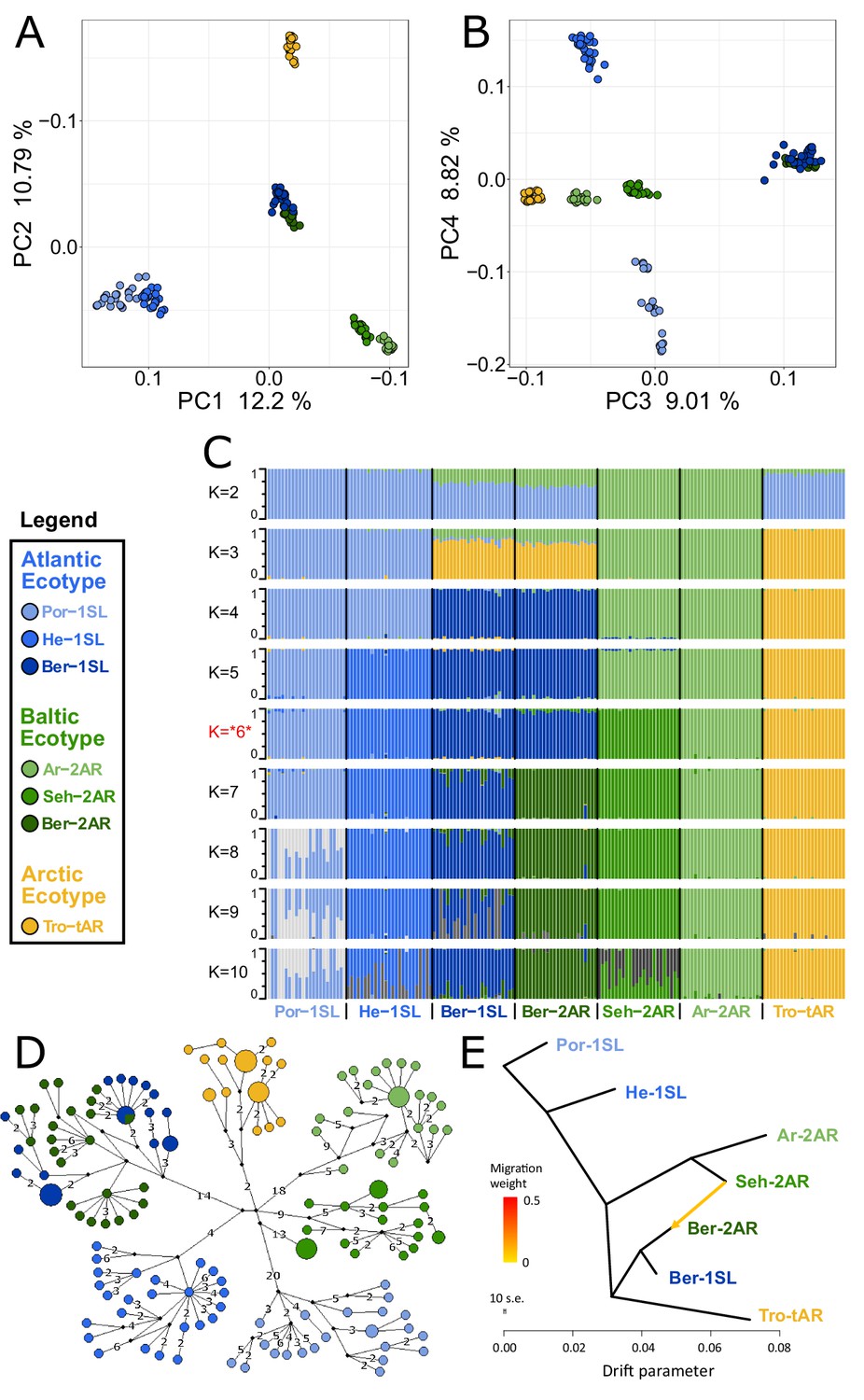
Genetic structure and evolutionary history of Northern European *Clunio* ecotypes.

The analysis is based on 24 individuals from each population (23 for Por-1SL, 25 for He-1SL). (**A, B**) Principal Component Analysis (PCA) based on 792,032 SNPs separates populations by geographic location rather than ecotype. (C) ADMIXTURE analysis supports strong differentiation by geographic site (best K=6), but a notable genetic component from the Baltic Sea in the Bergen populations (see K=2 and 3). The Bergen populations are only separated at K=7 and then show a number of admixed individuals. (D) Haplotype network of full mitochondrial genomes reveals highly divergent clusters according to geographic site, but haplotype sharing between Ber-1SL and Ber-2AR. (E) Correlated allele frequencies indicate introgression from Seh-2AR into Ber-2AR.

First, there is strong geographic isolation between populations from different sites. In PCA, clusters are formed according to geography (Figure 2A–B, Figure 2—figure supplement 1). Mitochondrial haplotypes are not shared and are diagnostically different between geographic sites (Figure 2D). In ADMIXTURE, the optimal number of genetic groups is six (Figure 2C, Figure 2—figure supplement 2), corresponding to the number of geographic sites, and there is basically no mixing between the six clusters (Figure 2C; K=6). Finally, there is isolation by distance (IBD; Figure 2—figure supplement 3).

Second, the sympatric ecotypes in Bergen are genetically very similar. In PCA they are not separated in the first four principal components (Figure 2A–B) and they are the only populations that share mitochondrial haplotypes (Figure 2D). In the ADMIXTURE analysis, they are only distinguished at K=7, a value larger than the optimal K. As soon as the two populations are distinguished, some individuals show signals of admixed origin (Figure 2C; K=7), compatible with the assumption of ongoing gene flow and incomplete reproductive isolation. These observations question the species status of C. balticus, which was based on the assumption of temporal isolation between these two populations (Heimbach, 1978).

Third, the data suggest that after the ice age Clunio colonized northern Europe from a single source and expanded along two fronts into the Baltic Sea and into the high Arctic. The mitochondrial haplotype network expands from a single center, which implies a quick radiation from a colonizing haplotype (Figure 2D; note that all sampled populations occur in areas under a former ice shield cover). There is also a large degree of shared nuclear polymorphisms. Thirty-four percent of polymorphic SNPs are polymorphic in all seven populations and 93% are polymorphic in at least two populations (Figure 2—figure supplement 4). Separation of the Baltic Sea populations along PC1 and the Arctic population along PC2 (Figure 2A), suggests that Clunio expanded into the high Arctic and into the Baltic Sea independently. Congruently, nucleotide diversity significantly decreases toward both expansion fronts (Figure 2—figure supplement 5, Supplementary file 1). Postglacial establishment from a common source indicates that the Baltic and Arctic ecotypes have evolved their new local adaptations during this expansion time, that is, in less than 10,000 years.

Fourth, ADMIXTURE analysis reveals that sympatric co-existence of the Atlantic and Baltic ecotypes in Bergen likely results from introgression of Baltic ecotype individuals into an existing Atlantic ecotype population. At K=2 and K=3 the two Baltic Sea populations Seh-2AR and Ar-2AR are separated from all other populations and the two Bergen populations Ber-2AR and Ber-1SL show a marked genetic contribution coming from these Baltic Sea populations (Figure 2C). The Baltic genetic component is slightly larger for the Baltic ecotype Ber-2AR population than for the Atlantic ecotype Ber-1SL population. A statistical analysis via TreeMix detects predominantly an introgression from Seh-2AR into Ber-2AR (Figure 2E, Figure 2—figure supplements 6 and 7), suggesting that haplotypes that convey the Baltic ecotype have introgressed into a population of Atlantic ecotype, resulting in the now observed sympatric co-existence of Baltic and Atlantic ecotypes in Bergen. So far Bergen is the only site for which sympatric co-existence of the ecotypes is known. Further work will be required to see if there is a larger area of overlap, for example in the Skagerrak, and if we see similar signals of introgression or possibly secondary contact in other sympatric populations.

While our observation adds to the evidence for a role of introgression in adaptation and early speciation processes (Edelman and Mallet, 2021; Baack and Rieseberg, 2007), it also constitutes an excellent starting point for mapping loci that could be involved in the respective ecotype adaptations. Under the assumption that fast adaptation and ecotype formation are mostly based on frequency changes in standing variation, one expects that the respective haplotypes should be shared between ecotypes, especially when transferred via introgression. The following analysis is focussed on the Atlantic and Baltic ecotypes, represented by three populations each.

Nuclear haplotype sharing

First, we reconstructed the genealogical relationship between 36 individuals (six from each population) in 50 kb windows (n=1,607) along the genome, followed by topology weighting. There are 105 possible unrooted tree topologies for six populations, and 46,656 possibilities to pick one individual from each population out of the set of 36. For each window along the genome, we assessed the relative support of each of the 105 population tree topologies by all 46,656 combinations of six individuals. We found that tree topologies change rapidly along the chromosomes (Figure 3A; Figure 3—figure supplement 1; Supplementary file 2). The tree topology obtained for the entire genome (Figure 3—figure supplement 2) dominates only in few genomic windows (Figure 3A, black bars ‘Orig.’), while usually one or several other topologies account for more than 75% of the tree topologies (Figure 3A, gray bars ‘Misc.’). Hardly ever do all combinations of six individuals follow a single population tree topology (Figure 3A, stars), which implies that in most genomic windows some individuals do not group with their population. Taken together, this indicates a massive sharing of haplotypes across populations.

Figure 3 with 12 supplements see all

Download asset Open asset

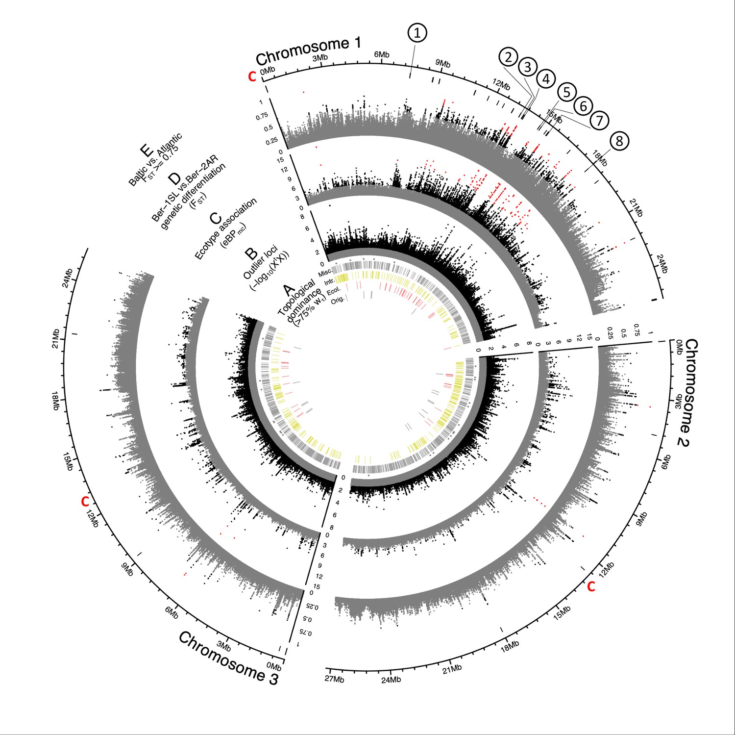
Genome screens for haplotype sharing and genotype-ecotype associations.

(A) Topology weighting of phylogenetic trees for 36 individuals from the *Baltic* and *Atlantic ecotypes*, as obtained from 50 kb non-overlapping genomic windows. Windows were marked by a bar if they were dominated by one kind of topology (w_τ>75%). Most windows are not dominated by the consensus population topology (‘Orig.’; Figure 3—figure supplement 2), but by combinations of other topologies (‘Misc.’). Windows dominated by topologies that separate the *Baltic* and *Atlantic ecotypes* (‘Ecol.’) are mostly on chromosome 1. Windows consistent with introgression are found all over the genome (‘Intr.’). (B) Distribution of outlier variants (SNPs and Indels) between the six *Baltic* and *Atlantic ecotype* populations, after global correction for population structure (X^tX statistic). Values below the significance threshold (as obtained by subsampling) are plotted in gray. (C) Association of variant frequencies with *Baltic* vs. *Atlantic ecotype* (eBP_mc). Values below the threshold of 3 (corresponding to p=10^–3) are given in gray, values above 10 are given in red. (D) Genetic differentiation (F_ST) between the sympatric ecotypes in Bergen. Values above 0.5 are given in black, values above 0.75 in red. (E) The distribution of SNPs with F_ST ≥ 0.75 in the *Baltic* vs. *Atlantic ecotypes*. Circled numbers mark the location of the eight most differentiated loci (see Figure 6). Centromeres of the chromosomes are marked by a red ‘C’.

In order to test whether this is only incomplete lineage sorting or if there is additional introgression beyond the detected case in the Bergen populations, we calculated the f4 ratio test for the geographically distant Por-1SL and He-1SL, as well as Ar-2AR and Seh-2AR populations. The genome-wide f4 ratio was –0.00062 (standard error 0.00008) and by comparison to coalescent simulations was found to be significantly different from 0, indicating some degree of introgression. However, the signature of introgression was driven by only 775 SNPs, which is only 0.17% of the total dataset. Thus, the largest part of haplotype sharing can be explained by incomplete lineage sorting, typical for such radiation situations.

Finally, we highlighted genomic windows that are consistent with the one clearly detected introgression event from the Baltic ecotype into both Bergen populations (Figure 3A, yellow bars ‘Intr.’; all topologies grouping Por-1SL and He-1SL vs Ber-1SL, Ber-2AR, Seh-2AR, and Ar-2AR; n=357). Regions consistent with this introgression event are scattered over the entire genome.

Crosses and QTL mapping suggest that lunar rhythmicity is affected by more than one locus (Fig. 4)

As a first attempt to get hold of ecologically relevant loci, we assessed the genetic basis to lunar rhythmicity by crossing the lunar-arrhythmic Ber-2AR strain with the lunar-rhythmic Ber-1SL strain. Interestingly, the degree of lunar rhythmicity segregates within and between crossing families (Figure 4—figure supplement 1), suggesting a heterogeneous multi-genic basis of lunar arrhythmicity. Genetic segregation in the cross implies that the weak rhythm observed in Ber-2AR is due to genetic polymorphism. The Ber-2AR strain seems to carry some lunar-rhythmic alleles, likely due to gene flow from the sympatric Atlantic ecotype (see Figure 1C and results below).

For QTL mapping, we then picked a set of F2 families, which all go back to a single parental pair (BsxBa-F2-34; n=272; Figure 4—figure supplement 1) and designed a set of 23 SNP markers for QTL mapping (Figure 4—figure supplement 2). As a phenotype, we scored the degree of lunar rhythmicity for each individual as the number of days between the individual’s emergence and day 9 of the artificial turbulence cycle, which is the peak emergence day of the lunar-rhythmic strain (Figure 4—figure supplement 3). However, QTL analysis with various algorithms did not reveal any significant QTL for lunar rhythmicity (Figure 4). This absence of evidence may partially be due to the limited number of markers and individuals, as well as a specific shortcoming in the phenotyping. Arrhythmic individuals, which by chance emerge during the peak, are recorded as rhythmic. This leads to an inevitable phenotyping error for a fraction of individuals. However, in another study, we could show that this phenotyping error does not impede the detection of an oligogenic genetic architecture in QTL mapping for a comparable arrhythmic phenotype (Briševac et al., 2022). As a control that in principle we had sufficient power for QTL mapping in this crossing family, we also mapped the sex determining locus, which was clearly detectable (Figure 4). We can conclude that lunar rhythmicity is not controlled by a single large-effect locus, but rather has an oligogenic or possibly even polygenic basis.

Figure 4 with 3 supplements see all

Download asset Open asset

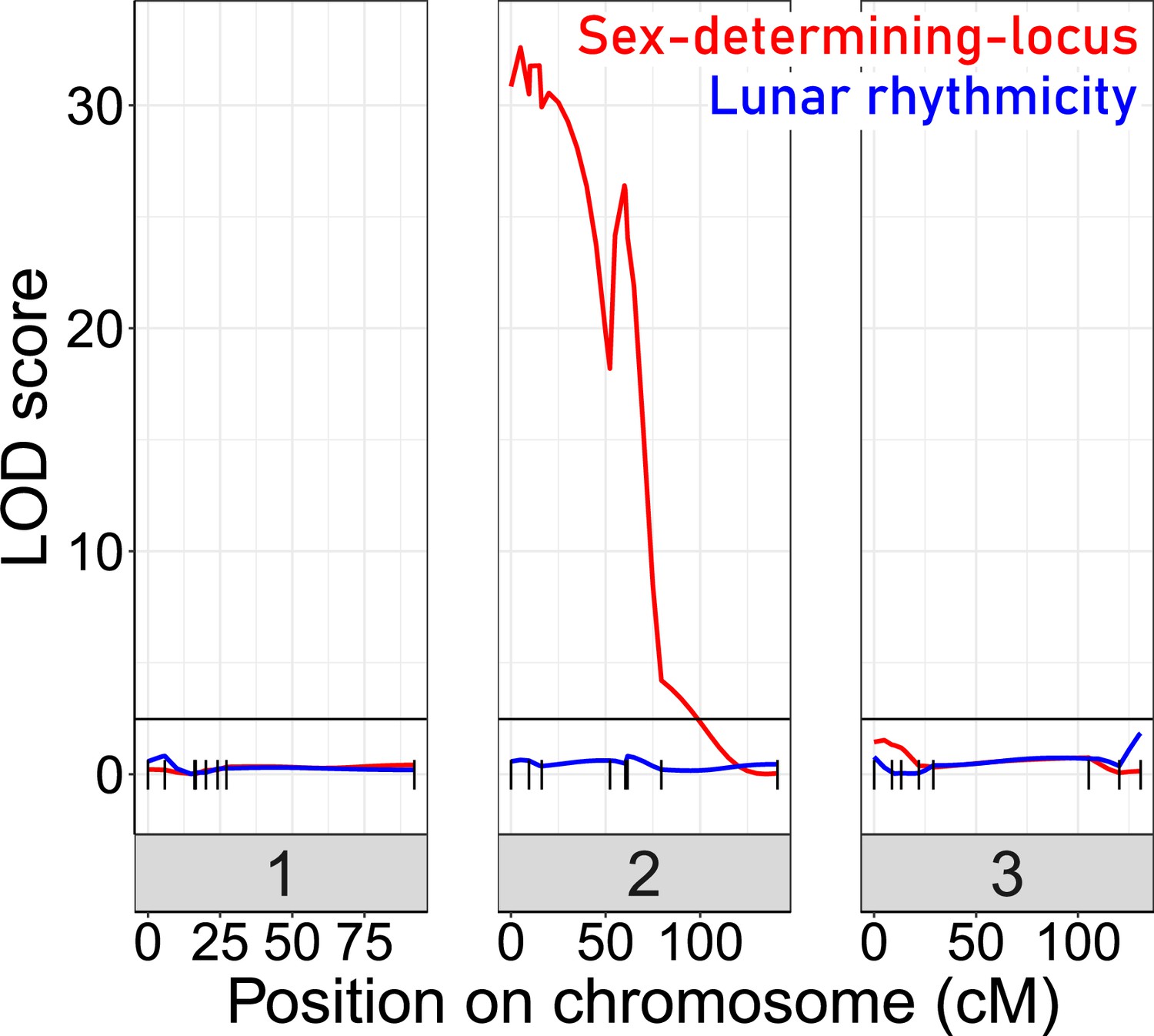
Quantitative Trait Locus (QTL) mapping for lunar rhythmicity (blue) and the sex determining locus (red).

The sex-determining locus is clearly detectable (red). No significant QTLs can be detected for lunar rhythmicity, suggesting it is controlled by more than one locus. Vertical black lines are genetic markers.

Genomic regions associated with ecotype formation

Given that QTL mapping for lunar rhythmicity suggested a multi-genic basis to ecotype formation, we next applied three approaches to identify genomic regions associated with divergence between Atlantic and Baltic ecotypes.

First, genomic windows which are dominated by tree topologies that group populations according to ecotype were highlighted (Figure 3A, red bars ‘Ecol.’).

Second, we screened all genetic variants (SNPs and indels; n=948,128) for those that are overly differentiated between the six populations after correcting for the neutral covariance structure across population allele frequencies (see $Ω$ matrix, Figure 3—figure supplement 3A–B). Such variants can indicate local adaptation. At the same time, we tested for association of these variants with ecotype, as implemented in BayPass Gautier, 2015. Overly differentiated variants (X^tX statistic; Figure 3B) and ecotype-associated variants ecotype (eBP_mc; Figure 3C) were detected all over the genome, but many were concentrated in the middle of the telocentric chromosome 1. Tests for association of variants with environmental variables such as sea surface temperature or salinity find fewer associated SNPs and no concentration on chromosome 1 (Figure 3—figure supplement 3D–E), confirming that the detected signals are not due to general genome properties, but are specific to the ecotypes.

Third, we expected that gene flow between the sympatric Ber-1SL and Ber-2AR populations would largely homogenize their genomes except for regions involved in ecological adaptation, which would be highlighted as peaks of genetic differentiation. While genetic differentiation may not only be due to adaptation, but also due to demographic processes, the ecologically relevant loci should be among the differentiated loci, especially if these loci coincide with peaks in ecotype-association (eBP_mc). The distributions of F_ST values in all pairwise population comparisons confirmed that genetic differentiation was particularly low in the Ber-1SL vs. Ber-2AR comparison (Figure 3—figure supplements 4 and 5). Pairwise differentiation between Ber-1SL and Ber-2AR (Figure 3D) shows marked peaks on chromosome 1, most of which coincide with peaks in X^tX and eBP_mc. Notably, when assessing genetic differentiation of Baltic vs Atlantic ecotype (72 vs 72 individuals; Figure 3E; Figure 3—figure supplement 6), there is not a single diagnostic variant (F_ST = 1), and even variants with F_ST ≥ 0.75 are very rare (n=63; Figure 3E).

Genetic divergence (d_xy), nucleotide diversity ( $π$ ) and local linkage disequilibrium (r²) of the two Bergen populations do not show marked differences along or between chromosomes (Figure 3—figure supplement 7). The cluster of ecotype-associated variants on chromosome 1 overlaps with three large blocks of long-range linkage disequilibrium (LD; Figure 3—figure supplement 8). This is also reflected in reduced linkage map length in our crossing mapping family (Figure 4—figure supplement 2). Reduced recombination may in part explain the clustering of divergent and ecotype-associated alleles in the middle of chromosome 1. However, the boundaries of the LD blocks do not correspond to the ecotype-associated region and differ between populations. LD blocks are not ecotype-specific. Local PCA of the strongly ecotype associated region does not reveal patterns consistent with a chromosomal inversion or another segregating structural variant (Figure 3—figure supplement 9). Thus, there is no obvious link between the clustering of ecotype-associated loci and structural variation. Notably, genetic differentiation is not generally elevated in the ecotype-associated cluster on chromosome 1, as would be expected for a segregating structural variant, but drops to baseline levels in between ecotype-associated loci (Figure 3D).

Taken together, these observations imply that numerous genomic loci – inside and outside the cluster on chromosome 1 – are associated with ecological adaptation and none of these are differentially fixed between ecotypes. In line with QTL mapping, this virtually excludes the possibility that only one or few loci have driven the new ecotype formation, suggesting instead that ecotype formation is based on a complex polygenic architecture.

Support for adaptation from standing genetic variation

If, as assumed above, adaptation in these populations was indeed based mostly on standing genetic variation, one should find evidence of this in the data structure. We selected highly ecotype-associated SNPs (X^tX >1.152094, threshold obtained from randomized subsampling; eBP_mc >3; n=3,976; Figure 3—figure supplement 10A) and assessed to which degree these alleles are shared between the studied populations and other populations across Europe. Allele sharing between the Bergen populations is likely due to ongoing gene flow, and hence Bergen populations were excluded from the analysis. In turn, allele sharing between the geographically isolated Seh-2AR, Ar-2AR, Por-1SL, and He-1SL populations likely represents shared ancient polymorphism. Based on this comparison, we found that 82% of the ecotype-associated SNPs are polymorphic in both Atlantic and Baltic ecotypes, suggesting that the largest part of ecotype-associated alleles originates from standing genetic variation. We then retrieved the same genomic positions from published population resequencing data for Atlantic ecotype populations from Vigo (Spain) and St. Jean-de-Luz (Jean, southern France) Kaiser et al., 2016, an area that is potentially the source of postglacial colonization of all locations in this study. We found that 90% of the alleles associated with the Northern European ecotypes are also segregating in at least one of these southern populations, supporting the notion that adaptation in the North involves a re-assortment of existing standing genetic variation.

Ecotypes differ mainly in the circadian clock and nervous system development

In the light of a polygenic architecture for ecotype formation, we can expect that usually several genes of relevant physiological pathways are affected. This provides an ideal setting to identify the physiological processes underlying ecotype formation by enrichment analysis. Accordingly, we assessed how all ecotype-associated variants (SNPs and indels; X^tX >1.148764; eBP_mc >3, n=4,741; Figure 3—figure supplement 10B) relate to C. marinus’ genes. In a first step, we filtered the existing gene models in the CLUMA1.0 reference genome to those that are supported by transcript or protein evidence, have known homologues or PFAM domains, or were manually curated (filtered annotations provided in Supplementary file 3; 15, 193 gene models). Based on this confidence gene set, we then assessed the location of variants relative to genes, as well as the resulting mutational effects (SNPeff; Cingolani et al., 2012; Figure 3—figure supplement 11; statistics in Supplementary file 4). The vast majority of ecotype-specific variants are classified as intergenic modifier variants, suggesting that ecotype formation might primarily rely on regulatory mutations.

The ecotype-specific SNPs are found in and around 1,400 genes (Supplementary files 5 and 6). We transferred GO terms from other species to the Clunio confidence annotations based on gene orthology (5,393 genes; see Methods and Supplementary file 7). GO term enrichment analysis suggests that ecological adaptation prominently involves the circadian clock, supported by three of the top four GO terms (Figure 5A). In order to identify which genes drive GO term enrichment in the top 40 GO terms, we extracted the genes that harbour ecotype-associated SNPs (168 genes; Figure 5B; Supplementary file 8). We individually confirmed their gene annotations and associated GO terms. Clustering the resulting table by genes and GO terms reveals two dominant signatures (Figure 5B). Many GO terms are associated with circadian timing and are driven by a small number of genes, which include almost all core circadian clock genes (Figure 5B and C). As a second strong signal, almost half of the genes are annotated with biological processes involved in nervous system development (Figure 5B and C). GO term enrichment is also found for ecdysteroid metabolism, imaginal disc development, and gonad development (Figure 5). These processes of pre-pupal development are expected to be under circalunar clock control. The fact that circalunar clocks are responsive to moonlight and water turbulence (Neumann, 2014) renders the finding of GO term enrichment for ‘auditory behavior’ and ‘phototaxis’ interesting. Furthermore, many of the genes involved in nervous system development and sodium ion transport, also have GO terms that implicate them in light- and mechanoreceptor development, wiring or sensitivity (Supplementary file 7). With the exception of ‘response to hypoxia’ and possibly ‘sodium ion transmembrane transport’, there are very few GO terms that can be linked to the submerged larval habitat of the Baltic ecotype, which is usually low in salinity and can turn hypoxic in summer. There is a striking absence of GO terms involved in metabolic processes or immune system processes, despite these GO terms being annotated to 2634 genes or 185 genes, respectively.

Figure 5

Download asset Open asset

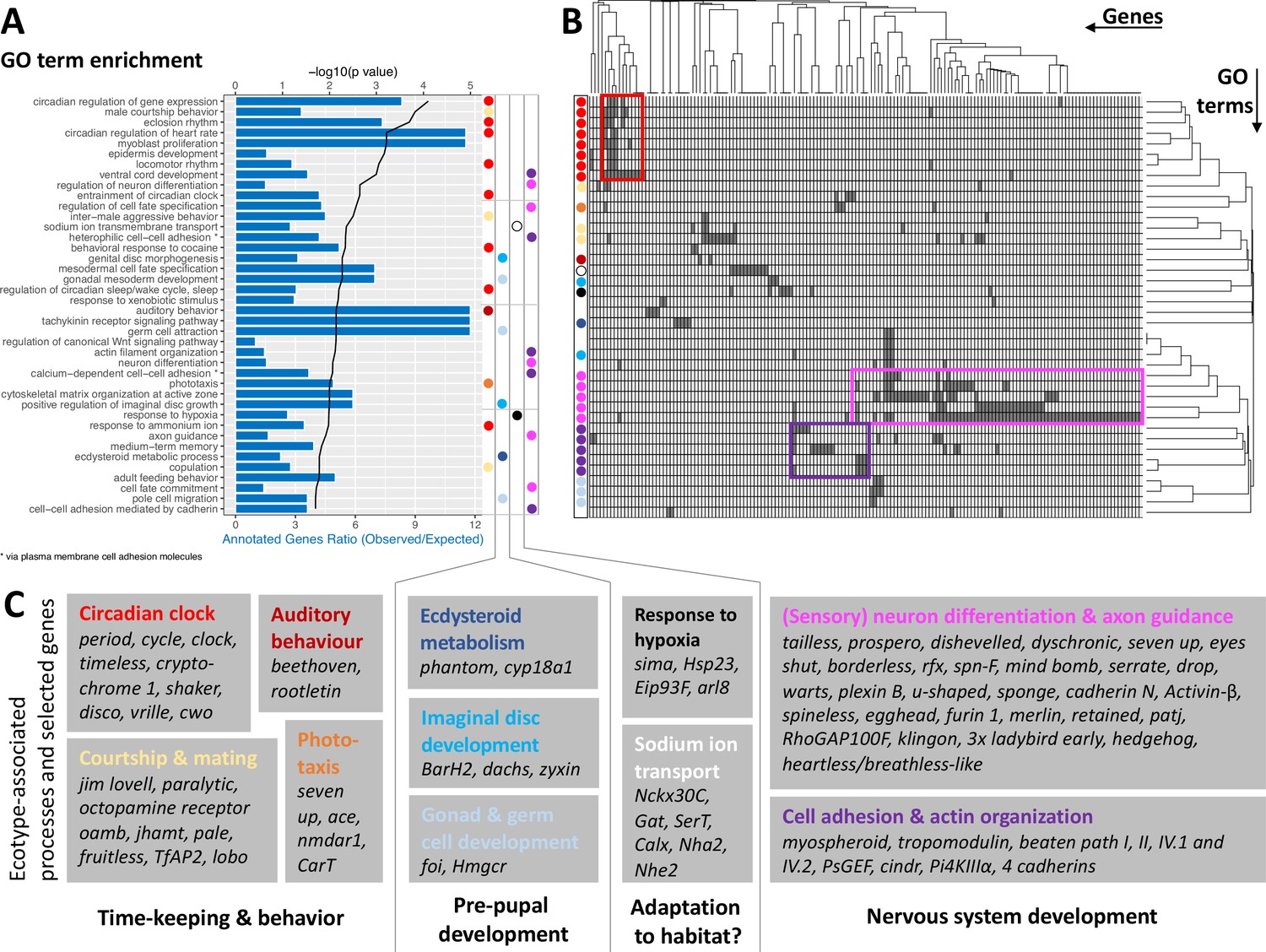
GO term analysis of ecotype associated SNPs (A) The top 40 enriched GO terms are listed for the 1,400 genes that are found to be affected by ecotype-associated genetic variants (eBP_mc >3).

For each GO term, the significance level (black line, top y-axis) and the observed-expected ratio of genes annotated to the respective GO term (blue bars, bottom y-axis) are given. (B) The top 40 GO terms are driven by 168 genes. Hierarchical clustering of genes and GO terms reveals major signals in the circadian clock and nervous system development (more details in Supplementary file 8). (C) Most GO terms are consistent with the known ecotype differences and selected genes are highlighted for all of them. Notably, basically all core circadian clock genes are affected.

Taken together, the detected GO terms are highly consistent with the known ecotype differences and suggest that ecotypes are mainly defined by changes in the circadian clock and nervous system development. A previously unknown aspect of Clunio ecotype formation is highlighted by the GO terms ‘male courtship behavior’, ‘inter-male aggression’ and ‘copulation’ (Figure 5). These processes are subject to sexual selection and considered to evolve rapidly. They could in the long term entail assortative mating between ecotypes.

Strongly differentiated loci correspond to GO-term enriched biological processes

While GO term analysis gives a broad picture of which processes have many genes affected by ecotype-associated SNPs, this does not necessarily imply that these genes and processes also show the strongest association with ecotype. Additionally, major genes might be missed because they were not assigned GO terms. As a second line of evidence, we therefore selected variants with the highest ecotype-association by increasing the eBP_mc cut-off to 10. This reduced the set of affected genes from 1,400 to 69 (Supplementary files 9 and 10). Additionally, we only considered genes with variants that are strongly differentiated between the ecotypes (F_ST ≥ 0.75, compare Figure 3E), leaving 13 genes in 8 distinct genomic regions (Figure 6A; numbered in Figure 3E). Two of these regions contain two genes each with no homology outside C. marinus (indicated by ‘NA’, Figure 6A), confirming that GO term analysis missed major loci because of a lack of annotation. Three other regions contain the – likely non-visual – photoreceptor ciliary Opsin 1 (cOps1) (Velarde et al., 2005), the transcription factor longitudinals lacking (lola; in fruit fly involved in axon guidance Crowner et al., 2002 and photoreceptor determination Zheng and Carthew, 2008) and the nuclear receptor tailless (tll; in fruit fly involved in development of brain and eye Suzuki and Saigo, 2000), underscoring that ecotype characteristics might involve differential light sensitivity. Interestingly, tll also affects development of the neuroendocrine centres involved in ecdysteroid production and adult emergence de Velasco et al., 2007. Even more, re-annotation of this genomic locus revealed that the neighbouring gene, which is also affected by ecotype-specific variants, is the short neuropeptide F receptor (sNPF-R) gene. Among other functions, sNPF-R is involved in coupling adult emergence to the circadian clock Selcho et al., 2017. Similarly, only 100 kb from cOps1 there is the differentiated locus of matrix metalloprotease 1 (Mmp1), which is known to regulate circadian clock outputs via processing of the neuropeptide pigment dispersing factor (PDF) Depetris-Chauvin et al., 2014. In both cases, the close genetic linkage could possibly form pre-adapted haplotypes and entail a concerted alteration of sensory and circadian functions in the formation of ecotypes. In the remaining two loci, sox100B is known to affect male gonad development Nanda et al., 2009 and the ecdysone-induced protein 93 F is involved in response to hypoxia in flies Lee et al., 2008, but was recently found to also affect reproductive cycles in mosquitoes Wang et al., 2021. In summary, only two out of the top 13 ecotype-associated genes were included in the top 40 GO terms (Figure 6A). Nevertheless, all major biological processes detected in GO term analysis (Figure 5) are also reflected in the strongly ecotype-associated loci (Figure 6), giving a robust signal that circadian timing, sensory perception and nervous system development are underlying ecotype formation in C. marinus.

Figure 6

Download asset Open asset

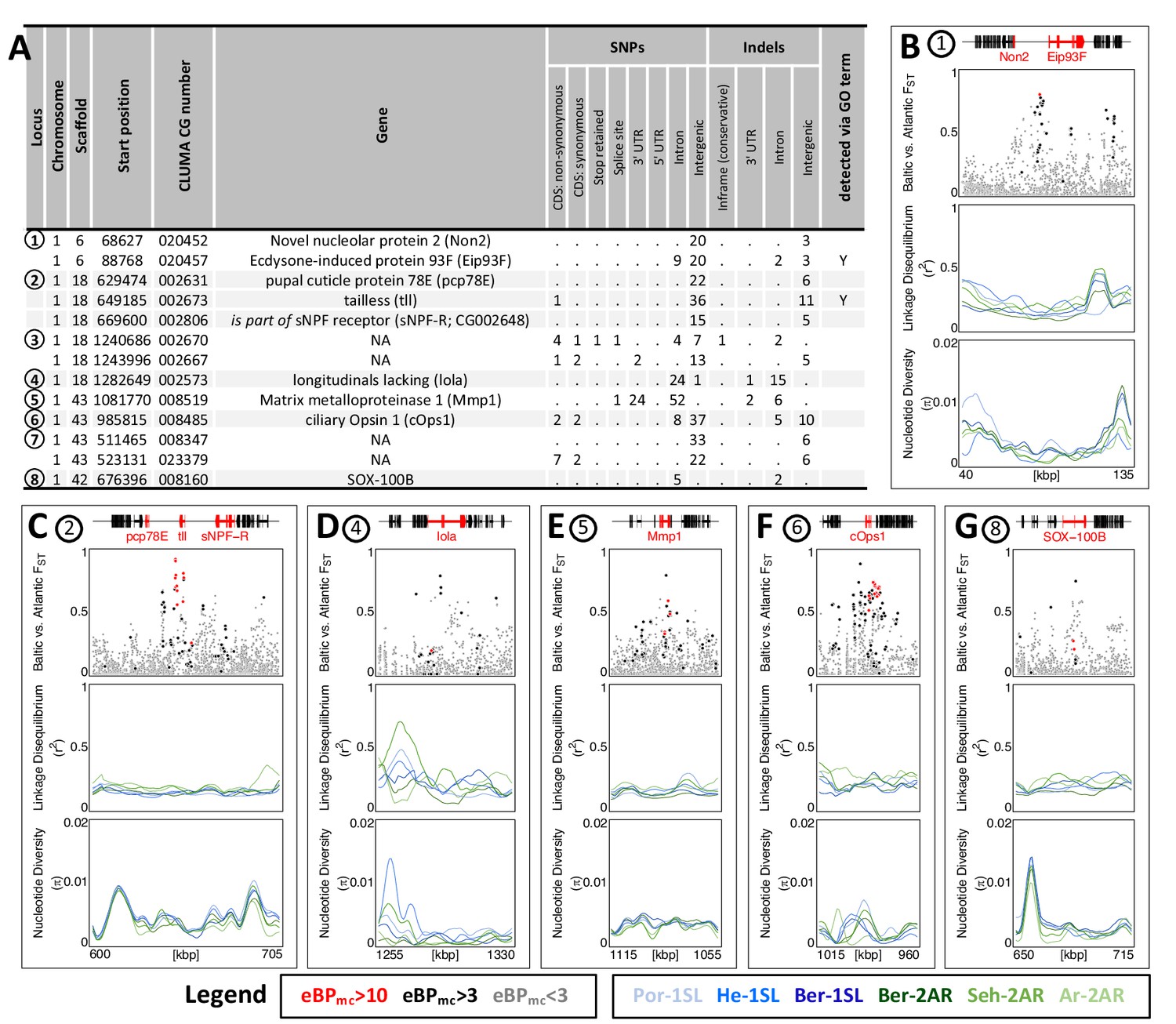
The 13 most differentiated ecotype-associated genes (A) Loci with highly ecotype-associated variants were selected based on eBPmc >10 and F_ST(Baltic-Atlantic)>0.75.

There are 13 genes in eight distinct genomic loci. (**B–G**) An overview is given for the six loci with identified genes. In each panel, from top to bottom the sub-panels show the gene models, F_ST values of genetic variants in the region, local linkage disequilibrium (LD) and genetic diversity ( $π$ ). F_ST values are colored by ecotype association of the variant (red: eBP_mc >10; black: 10>eBP_mc > 3; gray: eBP_mc <3). LD and genetic diversity are shown for the six populations independently, colored-coded as in Figures 1 and 2 (10 kb overlapping sliding-windows with 1 kb steps). The are no strong signatures of selection.

Figure 6—source data 1 Table of loci with highly ecotype-associated variants.: https://cdn.elifesciences.org/articles/82824/elife-82824-fig6-data1-v3.xlsx
Download elife-82824-fig6-data1-v3.xlsx

Finally, we assessed the top 13 strongly ecotype-associated loci for signatures of selective sweeps in genetic diversity and LD (Figure 6B–G). Despite these loci being the most differentiated between ecotypes in the entire genome, there is at best a mild reduction in genetic diversity and a mild increase in LD (Figure 6B–G). If selection acted on these loci, it must have been very soft, underscoring a history of polygenic adaptation from standing genetic variation and continued recombination.

Discussion

The deep genomic analysis of Clunio populations has allowed us to reconstruct a detailed biogeographic history of their different ecotypes. Most surprisingly, the two sympatric ecotypes that were considered different species turned out to be the most closely related populations in the sample, testifying the high power of ecology in generating differential adaptation in the face of gene flow. The data allowed further to infer a polygenic architecture for ecotype formation. We found that while ecotype-associated alleles differ in allele frequency, they are largely shared between ecotypes, which suggests that adaptation primarily involves standing genetic variation from many different loci. A similar re-use of existing regulatory variation has been found in ecotype formation in sticklebacks Chan et al., 2010; Kingman, 2020; Verta and Jones, 2019 or mimicry in Heliconius butterflies Edelman et al., 2019. However, while in Heliconius alleles are shared over large evolutionary distances via introgression, Clunio ecotypes diverged recently from a common source, as is illustrated by massive and genome-wide shared polymorphism. Combined with the observation that many genes from the same biological processes have ecotype-associated alleles, this draws a picture of polygenic adaptation, involving many pre-existing alleles with probably small phenotypic effects. Particularly for adaptation in circadian timing this scenario is highly plausible. The ancestral Atlantic ecotype comprises many genetically determined circadian timing types that are adapted to the local tides (Kaiser, 2014; Neumann, 1967; Kaiser et al., 2016; Kaiser et al., 2021). Existing genetic variants conveying emergence at dusk were likely selected or re-assorted to form the Baltic ecotype’s highly concentrated emergence at dusk.

Besides circadian timing, the ecotypes differ in circalunar timing and oviposition behavior. In our study, the vast majority of GO terms and candidate genes is consistent with these functions, leaving little risk for evolutionary ‘story-telling’ based on individual genes or GO terms (Pavlidis et al., 2012). We propose that good congruence between known phenotypic differences and detected biological processes could be a hallmark of polygenic adaptation, as only polygenic adaptation is expected to leave a footprint in many genes of the same ecologically relevant biological process.

Based on our genomic comparison of lunar-rhythmic and lunar-arrhythmic ecotypes, we propose three not mutually exclusive hypotheses on molecular pathways involved in the unknown circalunar clock. Firstly, Clunio’s circalunar clock is known to tightly regulate ecdysteroid-dependent development and maturation just prior to pupation (Neumann and Spindler, 1991). Congruently, our screen identified ecotype-associated genes in the development of imaginal discs and genital discs, and in ecdysteroid metabolism. Lunar arrhythmicity may rely on an escape of these processes from circalunar clock control. Secondly, it has been hypothesized that circalunar clocks involve a circadian clock (Bünning and Müller, 1961) and such a mechanism has been experimentally confirmed in the midge Pontomyia oceana (Soong and Chang, 2012). Thus, the overwhelming circadian signal in our data might be responsible for both circadian timing adaptations and the loss of circalunar rhythms. Thirdly, Clunio’s circalunar clock is synchronized with the external lunar cycle via moonlight, as well as tidal cycles of water turbulence and temperature (Neumann, 2014). Our data suggests that sensory receptor development, wiring or sensitivity might differ between ecotypes. Interestingly, some Atlantic ecotype populations are insensitive to specific lunar time cues, either moonlight or mechanical stimulation by the tides (Kaiser, 2014). These pre-existing insensitivities may have been combined to form completely insensitive and hence lunar-arrhythmic ecotypes. This scenario would fit the general pattern of polygenic adaptation through a re-assortment of standing genetic variation, which emerges from our study.

In several species, genes involved in complex behavioral or ecological syndromes were found to be locked into supergenes by chromosomal inversions, for example in Heliconius butterfly mimicry (Joron et al., 2011) or reproductive morphs of the ruff (Küpper et al., 2016). While we observe a clustering of ecotype-associated alleles in Clunio, there is no obvious connection to an underlying structural variant (SV). Possibly, the SV is so complex that it did not leave an interpretable genomic signal. Alternatively, Clunio’s long history of genome rearrangements (Kaiser et al., 2016) may have resulted in a clustering of ecologically relevant loci without locking them into a single SV. Clustering could be stabilized by low recombination, consistent with the observed three LD blocks, which – while not ecotype-specific – all overlap with the differentiated region. Epistatic interactions between the clustered loci and co-adaptation of alleles might further reduce the fitness of recombinants and lead to a concerted response to selection. Such an interconnected adaptive cluster might allow for more flexible evolutionary responses than a single, completely linked supergene. Further studies will have to show whether such a genome architecture exists, whether it facilitates adaptation and whether it might itself be selected for. Notably, a similar architecture with clustered, tightly linked loci was predicted to result from adaptation with gene flow (Yeaman and Whitlock, 2011), a scenario which we found in the sympatric Bergen populations.

Methods

Nomenclature of ecotypes

We expanded the existing naming convention of C. marinus timing types Kaiser et al., 2021 to also include Baltic and Arctic ecotypes. Names of populations and corresponding laboratory strains consist of an abbreviation for geographic origin followed by a code for the daily and lunar timing phenotypes. Daily phenotypes in this study are emergence during the first 12 hr after sunrise (‘1’) or, emergence during the second 12 hr after sunrise (‘2’) or emergence during every low tide (‘t’ for tidal rhythm). Lunar phenotypes in this study are either emergence during full moon and new moon low tides (‘SL’ for semi-lunar) or arrhythmic emergence (‘AR’). As a consequence, the Arctic ecotype is ‘tAR’, the Baltic ecotype is ‘2AR’ and the Atlantic ecotype populations in this study are all of timing type ‘1SL’ (while other timing types exist within the Atlantic ecotype Kaiser et al., 2021).

Fieldwork and sample collection

Field samples for genetic analysis and establishment of laboratory strains were collected in Sehlendorf (Seh, Germany), Ar (Sweden), Tromsø (Tro, Norway), and Bergen (Ber, Norway) during eight field trips in 2017 and 2018 (Supplementary file 11). Field caught adult males for DNA extraction were directly collected in 99.98% ethanol and stored at –20 °C. Females are immobile and basically invisible in the field, unless found in copulation. Laboratory strains were established by catching copulating pairs in the field and transferring multiple fertilized egg clutches to the laboratory (Supplementary file 11). Samples and laboratory strains of the sympatric ecotypes in Bergen were collected at the same location but at different daytime. Additional samples and laboratory strains from Helgoland (He, Germany) and Port-en-Bessin (Por, France) were collected and described earlier Kaiser et al., 2016; Kaiser et al., 2021; Kaiser et al., 2010, but had previously not been subject to whole genome sequencing of individuals.

Laboratory culture and phenotyping of ecotypes

Laboratory strains were reared under standard conditions Neumann, 1966 at 20 °C with 16 hr of light and 8 hr of darkness. Atlantic and Arctic ecotype strains were kept in natural seawater diluted 1:1 with deionized water and fed with diatoms (Phaeodactylum tricornutum) and powdered nettles (Urtica sp.). The Baltic ecotype was kept in natural Sea water diluted 1:2 and fed with diatoms and powdered red algae (90%, Delesseria spp., 10% Ceramium spp., obtained from F. Weinberger and N. Stärck, GEOMAR, Kiel). For entrainment of the lunar rhythm all strains were provided with 12.4 hr tidal cycles of water turbulence (mechanically induced vibrations produced by an unbalanced motor, 50 Hz, roughly 30 dB above background noise, 6hr 10 min on, 6 hr 15 min off) (Neumann and Heimbach, 1979; Neumann, 1978).

Assignment of strains to ecotypes was confirmed based on their phenotypes as recorded in laboratory culture. Oviposition behavior was assessed during standard culture maintenance: Baltic ecotype eggs are generally found submerged at the bottom of the culture vessel, Atlantic and Arctic ecotype eggs are always found floating on the water surface or on the walls of the culture vessel (for details see next paragraph). Daily emergence times were recorded in 1 hr intervals by direct observation (Seh-2AR, Ar-2AR) or with the help of a fraction collector (Honegger, 1977) (Ber-1SL, Ber-2AR, Tro-tAR, Por-1SL, He-1SL; Figure 1—figure supplement 1). Lunar emergence times were recorded by counting the number of emerged midges in the laboratory cultures every day over several months and summing them up over several tidal turbulence cycles. Emergence data for He-1SL was taken from Neumann, 1983, emergence data for Por-1SL was taken from Briševac et al., 2022.

Assessment of oviposition behavior

Because of the lack of tides in the Baltic Sea, the Baltic ecotype cannot rely on the tides to expose the larval substrates for egg deposition. Therefore, in contrast to the Atlantic and Arctic ecotypes, the Baltic ecotype does not oviposit on exposed larval substrates, but on the water surface, from where the eggs sink to the bottom of the sea. This change in oviposition preference is accompanied by a specific behavioral change, namely the bending of the female’s abdomen down through the water surface Endraß, 1976b, which ensures that the egg masses are not caught in the water’s surface tension. In our laboratory culture, the animals are kept in plastic boxes with a constant water level, so that larval substrates are never exposed. Under these conditions, most of the Baltic ecotype’s egg masses will be found submerged at the bottom of the culture box, as expected. Very rarely egg masses are deposited on the walls or the lid of the box. The Atlantic and Arctic ecotypes will – in the absence of exposed larval substrates – also oviposit on the water surface. However, as they lack the characteristic banding of the female abdomen during oviposition, their egg masses will be trapped in the water’s surface tension and cannot sink to the bottom of the culture box. Their egg masses will always float on the water surface, usually with the female still sticking to the egg jelly. These floating egg masses often form aggregations on the water surface. We used these differences in where the egg clutches are found in our laboratory cultures to additionally confirm ecotype identity of our laboratory strains.

Crosses and quantitative trait locus (QTL) mapping

The Ber-1SL and Ber-2AR laboratory strains were subject to single-pair crossing after their emergence rhythms were synchronized by keeping them in separate, time-shifted LD regimes. Several F1 families were raised independently and the F1 siblings were allowed to mate freely in order to obtain bulk F2 families. Emergence distributions were recorded by collecting all emerged adults every day.

Bulk crossing family BsxBa-F2-34 (n=272) was selected for QTL mapping. DNA of the two parents and the F2 progeny was extracted with the QuickExtract DNA Extraction Solution (Lucigen, QE0905T) according to manufacturer’s protocol with modifications. Instead of vortexing before incubation, a pestle was used to grind the sample. In order to identify scorable markers for the genetically very similar strains, the two parents of the cross were subject to whole-genome sequencing. Raw reads were processed through our genotyping pipeline (described below), resulting in 656,368 detected variants, 53,097 of which were diagnostic for the grandparents. Based on the list of diagnostic markers, we picked eight evenly spaced regions (physical distance) on each chromosome for amplicon sequencing (Figure 4—figure supplement 2, Supplementary file 12). Multiplex PCR was performed with the QIAGEN Multiplex PCR Kit (206143) for each chromosome primer set separately (15 min at 95 °C; 40 cycles of 94 °C for 30 s, 57 °C for 90 s and 72 °C for 90 s; 72 °C for 10 min). Sequencing libraries were prepared with standard Illumina protocols and sequenced with 150 bp paired-end on the Illumina HiSeq3000 sequencer by the Max Planck Genome Centre (Cologne, Germany). Sequencing reads from independent runs were first merged to one read file for forward and reverse reads. Those files were again subject to our genotyping pipeline (described below) with the exception that the mapped reads in SAM format undergone a coverage capping of 40 using a custom python script and the VCF was filtered for a minimum minor allele frequency of 0.25 ('--maf 0.25') and a maximum proportion of missing data per locus of 30% ('--max-missing 0.7'). All markers that were not diagnostic for the parents were removed. In case genotypes differed within an amplicon, a consensus amplicon genotype was called by majority.

For QTL mapping, the degree of rhythmicity of an individual was recorded as the number of days between its emergence day and day 9, which is the peak of emergence in the rhythmic strain (Ber-1SL). The phenotyping has a specific, inevitable shortcoming: Arrhythmic individuals can also emerge during the peak days by chance, so that this small fraction of individuals is phenotyped as rhythmic while actually being arrhythmic. As the phenotype is not normally distributed (Kolmogorov-Smirnov test and the Shapiro-Wilk test of normality) it was treated as non-parametric. QTL scans were performed in the R package ‘qtl’ (Broman et al., 2003). The genome scans with different QTL models followed the calculation of conditional genotype probabilities in 5 cM distances and simulated genotypes from 64 imputations with the same distance. Both phenotypes (lunar rhythmicity, sex) were scanned for a single QTL model in the ‘scanone()’ function (method = ‘em’). Significance thresholds were set at top 5% of the logarithm of the odds (LOD) scores for 1000 permutations. The ‘stepwise.qtl()’ function for identification of multiple and interacting QTLs returned a null QTL model for lunar rhythmicity.

DNA extraction and whole genome sequencing

For each of the seven populations, 24 field caught males (23 for Por-1SL, 25 for He-1SL) were subject to whole genome sequencing. DNA was extracted from entire individuals with a salting out method (Reineke et al., 1998) and amplified using the REPLI-g Mini Kit (QIAGEN) according to the manufacturer’s protocol with volume modifications (Supplementary file 13). All samples were subject to whole genome shotgun sequencing at 15–20 x target coverage on an Illumina HiSeq3000 sequencer with 150 bp paired-end reads. Library preparation and sequencing were performed by the Max Planck Genome Centre (Cologne, Germany) according to standard protocols. Raw sequence reads are deposited at ENA under Accession PRJEB43766.

Sequence data processing, genotyping, and SNP filtering

Raw sequence reads were trimmed for adapters and base quality using Trimmomatic v.0.38 Bolger et al., 2014 with parameters 'ILLUMINACLIP:TruSeq3-PE-2.fa:2:30:10:8:true', 'LEADING:20', 'TRAILING:20', 'MINLEN:75'. Overlapping paired end reads were merged with PEAR v.0.9.10 Zhang et al., 2014, setting the minimum assembled sequence length to 75 bp and a capping quality score of 20. Assembled and unassembled reads were mapped with BWA-MEM Li, 2013 to the nuclear reference genome Kaiser et al., 2016 (ENA accession GCA_900005825.1) and the mitochondrial reference genome (ENA accession CVRI01023763.1) of C. marinus. Mapped reads were sorted, indexed, filtered for mapping quality (-q 20) and transformed to BAM format with SAMtools v.1.9 Li et al., 2009. Read group information was added with the AddOrReplaceReadGroups.jar v.1.74 script from the Picard toolkit (http://picard.sourceforge.net/) DePristo et al., 2011.

For the nuclear genome, SNP and insertion-deletion (indel) genotypes were called using GATK v.3.8–0-ge9d806836 McKenna et al., 2010. After initial genotype calling with the GATK HaplotypeCaller and the parameter ‘-stand_call_conf 30’, base qualities were recalibrated with the GATK BaseRecalibrator with ‘-knownSites’ and genotype calling was repeated on the recalibrated BAM files to obtain the final individual VCF files. Individual VCF files were combined using GATK GenotypeGVCFs. SNP and indel genotypes were filtered with VCFtools v.0.1.14 Danecek et al., 2011 to keep only biallelic polymorphisms (--max-alleles 2), with a minimum minor allele frequency of 0.02 (--maf 0.02), a minimum genotype quality of 20 (--minQ 20) and a maximum proportion of missing data per locus of 40% (--max-missing 0.6), resulting in 792,032 SNPs and 156,096 indels over the entire set of 168 individuals. For certain analyses indels were excluded with VCFtools (‘--remove-indels’).

Reads mapped to the mitochondrial genome were transformed into mitochondrial haplotypes as described in Fuhrmann and Kaiser, 2020.

Population genomic analyses

Mitochondrial haplotype networks were calculated using the Median-Joining algorithm Bandelt et al., 1999 with Network v.10.1.0.0 (fluxus-engineering.com).

Nuclear SNP genotypes were converted to PLINK format with VCFtools. SNPs were LD pruned with PLINK v.1.90b4 Chang et al., 2015 and parameters ‘--indep-pairwise 50 10 0.5’ as well as ‘--chr-set 3 no-xy no-mt --nonfounders’ (resulting in 445,385 SNPs). Principal Component Analysis (PCA) was performed in PLINK using the option ‘--pca’ with the options default settings. The pruned BED file from PLINK was used as input to ADMIXTURE v.1.3.0 Alexander and Lange, 2011, with which we assessed a series of models for K=1 to K=10 genetic components, as well as the corresponding cross-validation error (‘--cv’). Migration was further tested by converting the SNP data to TreeMix format with the vcf2treemix.sh script Ravinet, 2021 and running TreeMix 1.13 Pickrell and Pritchard, 2012 with default parameters and the southernmost Por-1SL as root population. Finally, in order to distinguish incomplete lineage sorting from introgression on a broader geographic scale, we calculated the f4 ratio test Reich et al., 2009 as implemented in the f4.py script Meyer et al., 2017 for the He-1SL, Por-1SL, Ar-2AR and Seh-2AR populations. Standard error was obtained by jack-knifing in blocks of 100 SNPs (-k 100). We tested if the observed f4 ratio was significantly different from zero by comparison to 1,000 coalescent simulations on a random subset of 1% of the pruned SNPs (n=4,453; -s 1000).

Population estimates along the chromosomes were calculated in 100 kb overlapping sliding-windows with 10 kb steps (Figure 3—figure supplement 7) or 10 kb overlapping sliding-windows with 1 kb steps (Figure 6). Nucleotide diversity ( $π$ ) was calculated for SNPs with VCFtools ‘--window-pi’. For the genome-wide average, calculations were repeated with 200 kb non-overlapping windows. Linkage disequilibrium (LD; as r²) was calculated in VCFtools with ‘--geno-r2’. Local LD was calculated with ‘--ld-window-bp 500’. Preliminary tests showed that local LD decays within a few hundred base pairs (Figure 3—figure supplement 12). For long range LD, minor allele frequency was filtered to 0.2 (‘--maf 0.2‘, resulting in 335,800 SNPs), only values larger 0.5 were allowed with ‘--min-r2 0.5’ and the ‘--ld-window-bp 500’ filter was removed. Pairwise F_ST was calculated with VCFtools ‘--weir-fst-pop’ option per SNP and in sliding windows. For calculation of genetic divergence (d_xy), allele frequencies were extracted with VCFtools ‘--freq’ and d_xy was estimated from allele frequencies according to Delmore et al., 2015.

Phylogenomics and topology weighting

Nuclear genome phylogeny was calculated for a random set of six individuals from each population, without Tro-tAR (n=36). We down-sampled to six individuals per population because the following topology weighting algorithm assesses all possible combinations of six individuals (i.e. one per population) in the sample. The number of combinations grows exponentially with the number of individuals and thus leads to immense run-times of the algorithm. For windowed phylogenies, the VCF file was subset into non-overlapping 50 kb windows using VCFtools ‘--from-bp --to-bp’. SNP genotypes were transformed into FASTA alignments of only informative sites with the vcf2phylip.py v.2.3 script Ortiz, 2019 and parameters ‘-m 1 p -f’. Heterozygous genotypes were represented by the respective IUPAC code for both bases. Whole genome and windowed phylogenies were calculated with IQ-TREE v.1.6.12 Nguyen et al., 2015 using the parameters ‘-st DNA -m MFP -keep-ident -redo’ for the windowed and ‘-st DNA -m MFP -keep-ident -bb 1000 -bnni -nt 10 -redo’ for the whole genome phylogenies. Topology weighting was performed on the windowed phylogenies with TWISST Martin and Van Belleghem, 2017 and the parameter ‘--method complete’.

Association analysis

Population-based association between genetic variants (SNPs and Indels) and ecotype, as well as environmental variables (Supplementary file 14) was assessed in BayPass v.2.2 Gautier, 2015. Allele counts were obtained with VCFtools option ‘--counts’. Analyzed covariates were ecotype, sea surface salinity (obtained from Hordoir et al., 2019) and average water temperature of the year 2020 (obtained from weather-atlas.com, accessed 27.04.2020; 16:38), as given in Supplementary file 14. BayPass was run with the MCMC covariate model. BayPass corrects for population structure via $Ω$ dissimilarity matrices, then calculates the X^tX statistics and finally assesses the approximate Bayesian p value of association (eBP_mc). To obtain a significance threshold for X^tX values, the data was randomly subsampled (100,000 genetic variants) and re-analyzed with the standard covariate model, as implemented in baypass_utils.R. All analyses we performed in three replicates (starting seeds 5,001, 24,306, and 1,855) and the median is shown.

SNP effects and GO term enrichment analysis

Gene annotations to the CLUMA1.0 reference genome Kaiser et al., 2016 were considered reliable if they fulfilled one of three criteria: (1) Identified ortholog in UniProtKB/Swiss-Prot or non-redundant protein sequences (nr) at NCBI or PFAM domain, as reported in Kaiser et al., 2016. (2) Overlap of either at least 20% with mapped transcript data or 40% with mapped protein data, as reported in Kaiser et al., 2016. (3) Manually annotated. This resulted in a 15,193 confidence genes models. The location and putative effects of the SNPs and indels relative to these confidence gene models were annotated using SnpEff 4.5 Cingolani et al., 2012 (build 2020-04-15 22:26, non-default parameter `-ud 0’). Gene Ontology (GO) terms were annotated with emapper-2.0.1. Huerta-Cepas et al., 2017 from the eggNOG 5.0 database Huerta-Cepas et al., 2019, using DIAMOND Buchfink et al., 2015, BLASTP e-value <1e⁻¹⁰ and subject-query alignment coverage of >60%. Conservatively, we only transferred GO terms with ‘non-electronic’ GO evidence from best-hit orthologs restricted to an automatically adjusted per-query taxonomic scope, resulting in 5,393 C. marinus gene models with GO term annotations. Enrichment of ‘Biological Process’ GO terms in the genes associated with ecotype-specific polymorphisms was assessed with the weight01 Fisher’s exact test implemented in topGO Alexa and Rahnenfuhrer, 2010 (version 2.42.0, R version 4.0.3). When constructing the topGOdata object, the 5393 gene models with GO terms were specified as the custom background universe by providing the gene list to the parameter ‘allGenes’ and the custom gene-to-GO mappings were supplied by providing eggNOG GO annotations of these genes to the parameter ‘gene2GO’. Out of the 1,400 ecotype-associated gene models 463 were annotated with GO terms and only those went into GO term enrichment analysis. The fractions of genes with missing GO terms among the ecotype-associated genes and the total genes do not differ significantly (chi square test, p=0.12), suggesting both gene sets are equally affected by missing GO terms. Any potential biases in the reduced gene universe are accounted for by calculating the probability of observing at least the same degree of overrepresentation of a GO term when 463 genes are randomly selected out of the specified gene universe of 5393 genes (as implemented with the Fisher’s exact test in topGO).

Figure preparation

Figures were prepared in R Crawley, 2007. Data were handled with the ‘data.table’ Dowle, 2020 and ‘plyr’ Wickham, 2011 packages. The map of Europe was generated using the packages ‘ggplot2’ Wickham, 2016 and ‘ggrepel’ Slowikowski, 2018, ‘maps’ Brownrigg et al., 2018 and ‘mapdata’ Becker et al., 2018. The map was taken from the CIA World DataBank II (http://www.evl.uic.edu/pape/data/WDB/). Circular plots were prepared using the R package ‘circlize’ Gu et al., 2014. Multiple plots were combined in R using the package ‘Rmisc’ Hope, 2013. The graphical editing of the whole genome phylogeny was done in Archeopteryx (http://www.phylosoft.org/archaeopteryx) Han and Zmasek, 2009. Final figure combination and graphical editing of the raw plot files was done in Inkscape. Neighbor Joining trees of the omega statistic distances from BayPass were created with the R package ‘ape’ Paradis and Schliep, 2019. In all plots, the order and orientation of scaffolds within the chromosomes follows the published genetic linkage map Kaiser et al., 2016.

Data availability

Sequencing data for field samples and mapping families are deposited at ENA under Accession PRJEB43766. Filtered genome annotations are given in Supplementary File 3. All other data are included in the manuscript as supplementary data files.

The following data sets were generated

(2022) European Nucleotide Archive
ID PRJEB43766. Baltic and Arctic Clunio, whole genome resequencing.

https://www.ebi.ac.uk/ena/browser/view/PRJEB43766

References

Software
1. Alexa A
2. Rahnenfuhrer J
(2010) TopGO: enrichment analysis for gene ontology
R Package Version 2.

https://bioconductor.org/packages/release/bioc/html/topGO.html
1. Alexander DH
2. Lange K
(2011) Enhancements to the admixture algorithm for individual ancestry estimation
BMC Bioinformatics 12:246.

https://doi.org/10.1186/1471-2105-12-246
- PubMed
- Google Scholar
1. Andreatta G
2. Tessmar-Raible K
(2020) The still dark side of the moon: molecular mechanisms of lunar-controlled rhythms and clocks
Journal of Molecular Biology 432:3525–3546.

https://doi.org/10.1016/j.jmb.2020.03.009
- PubMed
- Google Scholar
1. Baack EJ
2. Rieseberg LH
(2007) A genomic view of introgression and hybrid speciation
Current Opinion in Genetics & Development 17:513–518.

https://doi.org/10.1016/j.gde.2007.09.001
- PubMed
- Google Scholar
(1999) Median-joining networks for inferring intraspecific phylogenies
Molecular Biology and Evolution 16:37–48.

https://doi.org/10.1093/oxfordjournals.molbev.a026036
- PubMed
- Google Scholar
(2020) Polygenic adaptation: a unifying framework to understand positive selection
Nature Reviews. Genetics 21:769–781.

https://doi.org/10.1038/s41576-020-0250-z
- PubMed
- Google Scholar
1. Barton NH
(2022) The “new synthesis.”
PNAS 119:e2122147119.

https://doi.org/10.1073/pnas.2122147119
- PubMed
- Google Scholar
Software
(2018) Mapdata extra map databases
R Package.

https://cran.r-project.org/web/packages/mapdata/index.html
(2014) Trimmomatic: a flexible trimmer for illumina sequence data
Bioinformatics 30:2114–2120.

https://doi.org/10.1093/bioinformatics/btu170
- PubMed
- Google Scholar
(2017) An expanded view of complex traits: from polygenic to omnigenic
Cell 169:1177–1186.

https://doi.org/10.1016/j.cell.2017.05.038
- PubMed
- Google Scholar
Preprint
(2022) Genetic Analysis of a Phenotypic Loss in the Mechanosensory Entrainment of a Circalunar Clock
bioRxiv.

https://doi.org/10.1101/2022.10.12.511720
- Google Scholar
1. Broman KW
2. Wu H
3. Sen S
4. Churchill GA
(2003) R/QTL: QTL mapping in experimental crosses
Bioinformatics 19:889–890.

https://doi.org/10.1093/bioinformatics/btg112
- PubMed
- Google Scholar
Software
(2018) Maps: draw geographical maps
R Package.

https://cran.r-project.org/web/packages/maps/maps.pdf
(2015) Fast and sensitive protein alignment using diamond
Nature Methods 12:59–60.

https://doi.org/10.1038/nmeth.3176
- PubMed
- Google Scholar
1. Bünning E
2. Müller D
(1961) Wie messen organismen lunare zyklen?
Zeitschrift Für Naturforschung B 16:391–395.

https://doi.org/10.1515/znb-1961-0609
- Google Scholar
1. Chan YF
2. Marks ME
3. Jones FC
4. Villarreal G Jr
5. Shapiro MD
6. Brady SD
7. Southwick AM
8. Absher DM
9. Grimwood J
10. Schmutz J
11. Myers RM
12. Petrov D
13. Jónsson B
14. Schluter D
15. Bell MA
16. Kingsley DM
(2010) Adaptive evolution of pelvic reduction in sticklebacks by recurrent deletion of a pitx1 enhancer
Science 327:302–305.

https://doi.org/10.1126/science.1182213
- PubMed
- Google Scholar
1. Chang CC
2. Chow CC
3. Tellier LC
4. Vattikuti S
5. Purcell SM
6. Lee JJ
(2015) Second-generation PLINK: rising to the challenge of larger and richer datasets
GigaScience 4:7.

https://doi.org/10.1186/s13742-015-0047-8
- PubMed
- Google Scholar
1. Cingolani P
2. Platts A
3. Wang LL
4. Coon M
5. Nguyen T
6. Wang L
7. Land SJ
8. Lu X
9. Ruden DM
(2012) A program for annotating and predicting the effects of single nucleotide polymorphisms, snpeff: snps in the genome of Drosophila melanogaster strain w1118; iso-2; iso-3
Fly 6:80–92.

https://doi.org/10.4161/fly.19695
- PubMed
- Google Scholar
Book
1. Crawley MJ
(2007) The R Book
Chichester, UK: John Wiley & Sons Ltd.

https://doi.org/10.1002/9780470515075
- Google Scholar
1. Crowner D
2. Madden K
3. Goeke S
4. Giniger E
(2002) Lola regulates midline crossing of CNS axons in Drosophila
Development 129:1317–1325.

https://doi.org/10.1242/dev.129.6.1317
- PubMed
- Google Scholar
(2011) The variant call format and vcftools
Bioinformatics 27:2156–2158.

https://doi.org/10.1093/bioinformatics/btr330
- PubMed
- Google Scholar
1. Delmore KE
2. Hübner S
3. Kane NC
4. Schuster R
5. Andrew RL
6. Câmara F
7. Guigó R
8. Irwin DE
(2015) Genomic analysis of a migratory divide reveals candidate genes for migration and implicates selective sweeps in generating islands of differentiation
Molecular Ecology 24:1873–1888.

https://doi.org/10.1111/mec.13150
- PubMed
- Google Scholar
(2014) Mmp1 processing of the PDF neuropeptide regulates circadian structural plasticity of pacemaker neurons
PLOS Genetics 10:e1004700.

https://doi.org/10.1371/journal.pgen.1004700
- PubMed
- Google Scholar
1. DePristo MA
2. Banks E
3. Poplin R
4. Garimella KV
5. Maguire JR
6. Hartl C
7. Philippakis AA
8. del Angel G
9. Rivas MA
10. Hanna M
11. McKenna A
12. Fennell TJ
13. Kernytsky AM
14. Sivachenko AY
15. Cibulskis K
16. Gabriel SB
17. Altshuler D
18. Daly MJ
(2011) A framework for variation discovery and genotyping using next-generation DNA sequencing data
Nature Genetics 43:491–498.

https://doi.org/10.1038/ng.806
- PubMed
- Google Scholar
1. de Velasco B
2. Erclik T
3. Shy D
4. Sclafani J
5. Lipshitz H
6. McInnes R
7. Hartenstein V
(2007) Specification and development of the pars intercerebralis and pars lateralis, neuroendocrine command centers in the Drosophila brain
Developmental Biology 302:309–323.

https://doi.org/10.1016/j.ydbio.2006.09.035
- PubMed
- Google Scholar
Software
1. Dowle M
(2020) Extension of ‘data. frame, version version 1.13.2
Package ‘Data.Table.’.

https://github.com/Rdatatable/data.table
1. Edelman NB
2. Frandsen PB
3. Miyagi M
4. Clavijo B
5. Davey J
6. Dikow RB
7. García-Accinelli G
8. Van Belleghem SM
9. Patterson N
10. Neafsey DE
11. Challis R
12. Kumar S
13. Moreira GRP
14. Salazar C
15. Chouteau M
16. Counterman BA
17. Papa R
18. Blaxter M
19. Reed RD
20. Dasmahapatra KK
21. Kronforst M
22. Joron M
23. Jiggins CD
24. McMillan WO
25. Di Palma F
26. Blumberg AJ
27. Wakeley J
28. Jaffe D
29. Mallet J
(2019) Genomic architecture and introgression shape a butterfly radiation
Science 366:594–599.

https://doi.org/10.1126/science.aaw2090
- PubMed
- Google Scholar
1. Edelman NB
2. Mallet J
(2021) Prevalence and adaptive impact of introgression
Annual Review of Genetics 55:265–283.

https://doi.org/10.1146/annurev-genet-021821-020805
- PubMed
- Google Scholar
1. Endraß U
(1976a) Physiologische anpassungen eines marinen insekts. I. die zeitliche steuerung der entwicklung
Marine Biology 34:361–368.

https://doi.org/10.1007/BF00398129
- Google Scholar
1. Endraß U
(1976b) Physiologische anpassungen eines marinen insekts. II. die eigenschaften von schwimmenden und absinkenden eigelegen
Marine Biology 36:47–60.

https://doi.org/10.1007/BF00388428
- Google Scholar
1. Field Y
2. Boyle EA
3. Telis N
4. Gao Z
5. Gaulton KJ
6. Golan D
7. Yengo L
8. Rocheleau G
9. Froguel P
10. McCarthy MI
11. Pritchard JK
(2016) Detection of human adaptation during the past 2000 years
Science 354:760–764.

https://doi.org/10.1126/science.aag0776
- PubMed
- Google Scholar
1. Fuhrmann N
2. Kaiser TS
(2020) The importance of DNA barcode choice in biogeographic analyses—a case study on marine midges of the genus clunio
Genome pp. 1–11.

https://doi.org/10.1139/gen-2019-0191
- Google Scholar
1. Gautier M
(2015) Genome-Wide scan for adaptive divergence and association with population-specific covariates
Genetics 201:1555–1579.

https://doi.org/10.1534/genetics.115.181453
- PubMed
- Google Scholar
1. Gu Z
2. Gu L
3. Eils R
4. Schlesner M
5. Brors B
(2014) Circlize implements and enhances circular visualization in R
Bioinformatics 30:2811–2812.

https://doi.org/10.1093/bioinformatics/btu393
- PubMed
- Google Scholar
1. Han MV
2. Zmasek CM
(2009) PhyloXML: XML for evolutionary biology and comparative genomics
BMC Bioinformatics 10:1–6.

https://doi.org/10.1186/1471-2105-10-356
- PubMed
- Google Scholar
1. Heimbach F
(1978) Sympatric species, Clunio marinus hal. and Cl. balticus n. sp. (dipt., chironomidae), isolated by differences in diel emergence time
Oecologia 32:195–202.

https://doi.org/10.1007/BF00366071
- Google Scholar
1. Hofmann W
2. Winn K
(2000) The littorina transgression in the western baltic sea as indicated by subfossil chironomidae (diptera) and cladocera (crustacea)
International Review of Hydrobiology 85:267–291.

https://doi.org/10.1002/(SICI)1522-2632(200004)85:2/3<267::AID-IROH267>3.0.CO;2-Q
- Google Scholar
1. Honegger HW
(1977)
An automatic device for the investigation of the rhythmic emergence pattern of clunio marinus

International Journal of Chronobiology 4:217–221.
- Google Scholar
Software
1. Hope RM
(2013) Rmisc: ryan miscellaneous
R Package.

https://cran.r-project.org/web/packages/Rmisc/Rmisc.pdf
1. Hordoir R
2. Axell L
3. Höglund A
4. Dieterich C
5. Fransner F
6. Gröger M
7. Liu Y
8. Pemberton P
9. Schimanke S
10. Andersson H
11. Ljungemyr P
12. Nygren P
13. Falahat S
14. Nord A
15. Jönsson A
16. Lake I
17. Döös K
18. Hieronymus M
19. Dietze H
20. Löptien U
21. Kuznetsov I
22. Westerlund A
23. Tuomi L
24. Haapala J
(2019) NEMO-nordic 1.0: a NEMO-based Ocean model for the Baltic and North seas – research and operational applications
Geoscientific Model Development 12:363–386.

https://doi.org/10.5194/gmd-12-363-2019
- Google Scholar
(2017) Fast genome-wide functional annotation through orthology assignment by eggnog-mapper
Molecular Biology and Evolution 34:2115–2122.

https://doi.org/10.1093/molbev/msx148
- PubMed
- Google Scholar
1. Huerta-Cepas J
2. Szklarczyk D
3. Heller D
4. Hernández-Plaza A
5. Forslund SK
6. Cook H
7. Mende DR
8. Letunic I
9. Rattei T
10. Jensen LJ
11. von Mering C
12. Bork P
(2019) EggNOG 5.0: a hierarchical, functionally and phylogenetically annotated orthology resource based on 5090 organisms and 2502 viruses
Nucleic Acids Research 47:D309–D314.

https://doi.org/10.1093/nar/gky1085
- PubMed
- Google Scholar
1. Joron M
2. Frezal L
3. Jones RT
4. Chamberlain NL
5. Lee SF
6. Haag CR
7. Whibley A
8. Becuwe M
9. Baxter SW
10. Ferguson L
11. Wilkinson PA
12. Salazar C
13. Davidson C
14. Clark R
15. Quail MA
16. Beasley H
17. Glithero R
18. Lloyd C
19. Sims S
20. Jones MC
21. Rogers J
22. Jiggins CD
23. ffrench-Constant RH
(2011) Chromosomal rearrangements maintain a polymorphic supergene controlling butterfly mimicry
Nature 477:203–206.

https://doi.org/10.1038/nature10341
- PubMed
- Google Scholar
(2010) Strong genetic differentiation and postglacial origin of populations in the marine midge clunio marinus (chironomidae, diptera)
Molecular Ecology 19:2845–2857.

https://doi.org/10.1111/j.1365-294X.2010.04706.x
- PubMed
- Google Scholar
(2011) Timing the tides: genetic control of diurnal and lunar emergence times is correlated in the marine midge clunio marinus
BMC Genetics 12:49.

https://doi.org/10.1186/1471-2156-12-49
- PubMed
- Google Scholar
1. Kaiser TS
2. Heckel DG
(2012) Genetic architecture of local adaptation in lunar and diurnal emergence times of the marine midge clunio marinus (chironomidae, diptera)
PLOS ONE 7:e32092.

https://doi.org/10.1371/journal.pone.0032092
- PubMed
- Google Scholar
Book
1. Kaiser T
(2014) Patterns and mechanisms of nature’s enigmatic rhythms
In: Numata B, editors. Annual, Lunar, and Tidal Clocks. Japan: Springer. pp. 121–141.

https://doi.org/10.1007/978-4-431-55261-1
- Google Scholar
1. Kaiser TS
2. Poehn B
3. Szkiba D
4. Preussner M
5. Sedlazeck FJ
6. Zrim A
7. Neumann T
8. Nguyen LT
9. Betancourt AJ
10. Hummel T
11. Vogel H
12. Dorner S
13. Heyd F
14. von Haeseler A
15. Tessmar-Raible K
(2016) The genomic basis of circadian and circalunar timing adaptations in a midge
Nature 540:69–73.

https://doi.org/10.1038/nature20151
- PubMed
- Google Scholar
(2021) Timing strains of the marine insect clunio marinus diverged and persist with gene flow
Molecular Ecology 30:1264–1280.

https://doi.org/10.1111/mec.15791
- PubMed
- Google Scholar
1. Kautt AF
2. Kratochwil CF
3. Nater A
4. Machado-Schiaffino G
5. Olave M
6. Henning F
7. Torres-Dowdall J
8. Härer A
9. Hulsey CD
10. Franchini P
11. Pippel M
12. Myers EW
13. Meyer A
(2020) Contrasting signatures of genomic divergence during sympatric speciation
Nature 588:106–111.

https://doi.org/10.1038/s41586-020-2845-0
- PubMed
- Google Scholar
Preprint
1. Kingman GAR
(2020) Predicting Future from Past: The Genomic Basis of Recurrent and Rapid Stickleback Evolution
bioRxiv.

https://doi.org/10.1101/2020.11.13.382424
- Google Scholar
1. Küpper C
2. Stocks M
3. Risse JE
4. Dos Remedios N
5. Farrell LL
6. McRae SB
7. Morgan TC
8. Karlionova N
9. Pinchuk P
10. Verkuil YI
11. Kitaysky AS
12. Wingfield JC
13. Piersma T
14. Zeng K
15. Slate J
16. Blaxter M
17. Lank DB
18. Burke T
(2016) A supergene determines highly divergent male reproductive morphs in the ruff
Nature Genetics 48:79–83.

https://doi.org/10.1038/ng.3443
- PubMed
- Google Scholar
1. Le Corre V
2. Kremer A
(2012) The genetic differentiation at quantitative trait loci under local adaptation
Molecular Ecology 21:1548–1566.

https://doi.org/10.1111/j.1365-294X.2012.05479.x
- PubMed
- Google Scholar
(2008) An RNA interference screen identifies a novel regulator of target of rapamycin that mediates hypoxia suppression of translation in Drosophila S2 cells
Molecular Biology of the Cell 19:4051–4061.

https://doi.org/10.1091/mbc.e08-03-0265
- PubMed
- Google Scholar
(2009) The sequence alignment/map format and samtools
Bioinformatics 25:2078–2079.

https://doi.org/10.1093/bioinformatics/btp352
- PubMed
- Google Scholar
Preprint
1. Li H
(2013) Aligning Sequence Reads, Clone Sequences and Assembly Contigs with BWA-MEM
arXiv.

https://doi.org/10.48550/arXiv.1303.3997
- Google Scholar
1. Martin SH
2. Van Belleghem SM
(2017) Exploring evolutionary relationships across the genome using topology weighting
Genetics 206:429–438.

https://doi.org/10.1534/genetics.116.194720
- PubMed
- Google Scholar
1. McKenna A
2. Hanna M
3. Banks E
4. Sivachenko A
5. Cibulskis K
6. Kernytsky A
7. Garimella K
8. Altshuler D
9. Gabriel S
10. Daly M
11. DePristo MA
(2010) The genome analysis toolkit: a mapreduce framework for analyzing next-generation DNA sequencing data
Genome Research 20:1297–1303.

https://doi.org/10.1101/gr.107524.110
- PubMed
- Google Scholar
(2017) Disentangling incomplete lineage sorting and introgression to refine species-tree estimates for lake tanganyika cichlid fishes
Systematic Biology 66:531–550.

https://doi.org/10.1093/sysbio/syw069
- PubMed
- Google Scholar
1. Nanda S
2. DeFalco TJ
3. Loh SHY
4. Phochanukul N
5. Camara N
6. Van Doren M
7. Russell S
(2009) Sox100B, a Drosophila group E sox-domain gene, is required for somatic testis differentiation
Sexual Development 3:26–37.

https://doi.org/10.1159/000200079
- PubMed
- Google Scholar
1. Neumann D
(1966)
Die lunare und tägliche schlüpfperiodik der Mücke clunio - steuerung und abstimmung auf die gezeitenperiodik

Zeitschrift Für Vergleichende Physiologie 53:1–61.
- Google Scholar
1. Neumann D
(1967) Genetic adaptation in emergence time ofclunio populations to different tidal conditions
Helgoländer Wissenschaftliche Meeresuntersuchungen 15:163–171.

https://doi.org/10.1007/BF01618620
- Google Scholar
1. Neumann D
2. Honegger HW
(1969) Adaptations of the intertidal midge clunio to Arctic conditions
Oecologia 3:1–13.

https://doi.org/10.1007/BF00344631
- PubMed
- Google Scholar
1. Neumann D
(1978) Entrainment of a semilunar rhythm by simulated tidal cycles of mechanical disturbance
Journal of Experimental Marine Biology and Ecology 35:73–85.

https://doi.org/10.1016/0022-0981(78)90091-6
- Google Scholar
Book
1. Neumann D
2. Heimbach F
(1979)
Cyclic Phenomena in Marine Plants and Animals

Elsevier.
- Google Scholar
Book
1. Neumann D
(1983) Die zeitliche programmierung von tieren auf periodische umweltbedingungen
In: Vorträge G, editors. Rheinisch-Westfälische Akademie Der Wissenschaften. Springer. pp. 31–62.

https://doi.org/10.1007/978-3-322-85974-7_2
- Google Scholar
1. Neumann D
2. Spindler KD
(1991) Circasemilunar control of imaginal disc development in clunio marinus: temporal switching point, temperature-compensated developmental time and ecdysteroid profile
Journal of Insect Physiology 37:101–109.

https://doi.org/10.1016/0022-1910(91)90095-H
- Google Scholar
Book
1. Neumann D
(2014) Circannual rhythms: history, present challenges, future directions
In: Numata H, Helm B, editors. Annual, Lunar, and Tidal Clocks. Japan: Springer. pp. 3–24.

https://doi.org/10.1007/978-4-431-55261-1_11
- Google Scholar
(2015) IQ-TREE: a fast and effective stochastic algorithm for estimating maximum-likelihood phylogenies
Molecular Biology and Evolution 32:268–274.

https://doi.org/10.1093/molbev/msu300
- PubMed
- Google Scholar
1. Nosil P
2. Schluter D
(2011) The genes underlying the process of speciation
Trends in Ecology & Evolution 26:160–167.

https://doi.org/10.1016/j.tree.2011.01.001
- PubMed
- Google Scholar
1. Orr HA
(1998) The population genetics of adaptation: the distribution of factors fixed during adaptive evolution
Evolution; International Journal of Organic Evolution 52:935–949.

https://doi.org/10.1111/j.1558-5646.1998.tb01823.x
- PubMed
- Google Scholar
Software
1. Ortiz E
(2019) Vcf2phylip v2.0: convert a VCF matrix into several matrix formats for phylogenetic analysis
Zenoda.

https://zenodo.org/record/2540861#.Y-XWjXZBw2w
1. Palmén E
2. Lindeberg B
(1959) The marine midge, clunio marinus hal. (dipt., chironomidae), found in brackish water in the northern baltic
Internationale Revue Der Gesamten Hydrobiologie Und Hydrogeographie 44:383–393.

https://doi.org/10.1002/iroh.19590440120
- Google Scholar
1. Paradis E
2. Schliep K
(2019) Ape 5.0: an environment for modern phylogenetics and evolutionary analyses in R
Bioinformatics 35:526–528.

https://doi.org/10.1093/bioinformatics/bty633
- PubMed
- Google Scholar
1. Patton H
2. Hubbard A
3. Andreassen K
4. Auriac A
5. Whitehouse PL
6. Stroeven AP
7. Shackleton C
8. Winsborrow M
9. Heyman J
10. Hall AM
(2017) Deglaciation of the Eurasian ice sheet complex
Quaternary Science Reviews 169:148–172.

https://doi.org/10.1016/j.quascirev.2017.05.019
- Google Scholar
(2012) A critical assessment of storytelling: gene ontology categories and the importance of validating genomic scans
Molecular Biology and Evolution 29:3237–3248.

https://doi.org/10.1093/molbev/mss136
- PubMed
- Google Scholar
1. Pflüger W
2. Neumann D
(1971) Die steuerung einer gezeitenparallelen schlüpfrhythmik nACh dem sanduhr-prinzip
Oecologia 7:262–266.

https://doi.org/10.1007/BF00345216
- PubMed
- Google Scholar
1. Phadnis N
2. Orr HA
(2009) A single gene causes both male sterility and segregation distortion in Drosophila hybrids
Science 323:376–379.

https://doi.org/10.1126/science.1163934
- PubMed
- Google Scholar
1. Pickrell J
2. Pritchard J
(2012) Inference of population splits and mixtures from genome-wide allele frequency data
Nature Precedings 1–1:.

https://doi.org/10.1038/npre.2012.6956.1
- Google Scholar
Software
1. Ravinet M
(2021) Speciationgenomics, version 48a9fb2
Github.

https://github.com/speciationgenomics/scripts/blob/master/vcf2treemix.sh
1. Reich D
2. Thangaraj K
3. Patterson N
4. Price AL
5. Singh L
(2009) Reconstructing Indian population history
Nature 461:489–494.

https://doi.org/10.1038/nature08365
- PubMed
- Google Scholar
(1998) Preparation and purification of DNA from insects for AFLP analysis
Insect Molecular Biology 7:95–99.

https://doi.org/10.1046/j.1365-2583.1998.71048.x
- Google Scholar
1. Remmert H
(1955)
Ökologische untersuchungen über die dipteren der nord- und ostsee

Archiv Für Hydrobiologie 51:1–53.
- Google Scholar
1. Robinson MR
2. Hemani G
3. Medina-Gomez C
4. Mezzavilla M
5. Esko T
6. Shakhbazov K
7. Powell JE
8. Vinkhuyzen A
9. Berndt SI
10. Gustafsson S
11. Justice AE
12. Kahali B
13. Locke AE
14. Pers TH
15. Vedantam S
16. Wood AR
17. van Rheenen W
18. Andreassen OA
19. Gasparini P
20. Metspalu A
21. van den Berg L
22. Veldink JH
23. Rivadeneira F
24. Werge TM
25. Abecasis GR
26. Boomsma DI
27. Chasman DI
28. de Geus EJC
29. Frayling TM
30. Hirschhorn JN
31. Hottenga JJ
32. Ingelsson E
33. Loos RJF
34. Magnusson PKE
35. Martin NG
36. Montgomery GW
37. North KE
38. Pedersen NL
39. Spector TD
40. Speliotes EK
41. Goddard ME
42. Yang J
43. Visscher PM
(2015) Population genetic differentiation of height and body mass index across europe
Nature Genetics 47:1357–1362.

https://doi.org/10.1038/ng.3401
- PubMed
- Google Scholar
1. Selcho M
2. Millán C
3. Palacios-Muñoz A
4. Ruf F
5. Ubillo L
6. Chen J
7. Bergmann G
8. Ito C
9. Silva V
10. Wegener C
11. Ewer J
(2017) Central and peripheral clocks are coupled by a neuropeptide pathway in Drosophila
Nature Communications 8:15563.

https://doi.org/10.1038/ncomms15563
- PubMed
- Google Scholar
1. Sella G
2. Barton NH
(2019) Thinking about the evolution of complex traits in the era of genome-wide association studies
Annual Review of Genomics and Human Genetics 20:461–493.

https://doi.org/10.1146/annurev-genom-083115-022316
- PubMed
- Google Scholar
Software
1. Slowikowski K
(2018) Automatically position non-overlapping text labels with ‘ggplot2
Package Ggrepel.

https://rdrr.io/cran/ggrepel/
1. Soong K
2. Chang YH
(2012) Counting circadian cycles to determine the period of a circasemilunar rhythm in a marine insect
Chronobiology International 29:1329–1335.

https://doi.org/10.3109/07420528.2012.728548
- PubMed
- Google Scholar
1. Suzuki T
2. Saigo K
(2000) Transcriptional regulation of atonal required for Drosophila larval eye development by concerted action of eyes absent, sine oculis and hedgehog signaling independent of fused kinase and cubitus interruptus
Development 127:1531–1540.

https://doi.org/10.1242/dev.127.7.1531
- PubMed
- Google Scholar
(2012) Evidence of widespread selection on standing variation in europe at height-associated snps
Nature Genetics 44:1015–1019.

https://doi.org/10.1038/ng.2368
- PubMed
- Google Scholar
1. Van’t Hof AE
2. Campagne P
3. Rigden DJ
4. Yung CJ
5. Lingley J
6. Quail MA
7. Hall N
8. Darby AC
9. Saccheri IJ
(2016) The industrial melanism mutation in British peppered moths is a transposable element
Nature 534:102–105.

https://doi.org/10.1038/nature17951
- PubMed
- Google Scholar
(2005) Pteropsin: a vertebrate-like non-visual opsin expressed in the honey bee brain
Insect Biochemistry and Molecular Biology 35:1367–1377.

https://doi.org/10.1016/j.ibmb.2005.09.001
- PubMed
- Google Scholar
1. Verta JP
2. Jones FC
(2019) Predominance of cis-regulatory changes in parallel expression divergence of sticklebacks
eLife 8:e43785.

https://doi.org/10.7554/eLife.43785
- PubMed
- Google Scholar
1. Wang X
2. Ding Y
3. Lu X
4. Geng D
5. Li S
6. Raikhel AS
7. Zou Z
(2021) The ecdysone-induced protein 93 is a key factor regulating gonadotrophic cycles in the adult female mosquito aedes aegypti
PNAS 118:e2021910118.

https://doi.org/10.1073/pnas.2021910118
- PubMed
- Google Scholar
1. Wickham H
(2011) The split-apply-combine strategy for data analysis
Journal of Statistical Software 40:1–29.

https://doi.org/10.18637/jss.v040.i01
- Google Scholar
1. Wickham H
(2016)
Ggplot2: Elegant Graphics for Data Analysis

Ggplot2, Ggplot2: Elegant Graphics for Data Analysis, Cham, springer, 10.1007/978-3-319-24277-4.
- Google Scholar
1. Wu CI
2. Ting CT
(2004) Genes and speciation
Nature Reviews. Genetics 5:114–122.

https://doi.org/10.1038/nrg1269
- PubMed
- Google Scholar
1. Yeaman S
2. Whitlock MC
(2011) The genetic architecture of adaptation under migration-selection balance
Evolution; International Journal of Organic Evolution 65:1897–1911.

https://doi.org/10.1111/j.1558-5646.2011.01269.x
- PubMed
- Google Scholar
(2014) Pear: a fast and accurate illumina paired-end read merger
Bioinformatics 30:614–620.

https://doi.org/10.1093/bioinformatics/btt593
- PubMed
- Google Scholar
1. Zheng L
2. Carthew RW
(2008) Lola regulates cell fate by antagonizing Notch induction in the Drosophila eye
Mechanisms of Development 125:18–29.

https://doi.org/10.1016/j.mod.2007.10.007
- PubMed
- Google Scholar

Article and author information

Author details

Nico Fuhrmann

Max Planck Institute for Evolutionary Biology, Plön, Germany

Contribution
Data curation, Formal analysis, Investigation, Visualization, Writing - review and editing, Field work

Competing interests
No competing interests declared
Celine Prakash

Max Planck Institute for Evolutionary Biology, Plön, Germany

Contribution
Formal analysis, Investigation, Visualization, Writing - review and editing

Competing interests
No competing interests declared
Tobias S Kaiser

Max Planck Institute for Evolutionary Biology, Plön, Germany

Contribution
Conceptualization, Resources, Formal analysis, Supervision, Funding acquisition, Investigation, Visualization, Writing – original draft, Project administration

For correspondence
kaiser@evolbio.mpg.de

Competing interests
No competing interests declared

"This ORCID iD identifies the author of this article:" 0000-0002-4126-0533

Funding

European Research Council (802923)

Tobias S Kaiser

Max-Planck-Gesellschaft

Tobias S Kaiser

The funders had no role in study design, data collection and interpretation, or the decision to submit the work for publication. Open access funding provided by Max Planck Society.

Acknowledgements

For field work we obtained logistic support from the Ar Research Station (Uppsala University), the Marine Biological Station Espegrend (University of Bergen), Even Jørgensen (The Arctic University of Norway, Tromsø) and Florian Weinberger and Nadja Stärck (GEOMAR Helmholtz Centre for Ocean Research, Kiel). We thank Jürgen Reunert, Kerstin Schäfer and Susanne Mentz for technical assistance, as well as all members of the MPRG “Biological Clocks” for discussion and support. Diethard Tautz and Julien Dutheil critically read the manuscript. Whole genome sequencing was performed at the Max Planck Genome Center (Cologne) with financial support from the Max Planck Society. This work was funded by the Max Planck Society through the Max Planck Research Group “Biological Clocks” and a sequencing grant. The work was further funded by the European Research Council (ERC) under the Horizon 2020 research and innovation program with an ERC Starting Grant (Grant agreement 802923) awarded to TSK.

Copyright

This article is distributed under the terms of the Creative Commons Attribution License, which permits unrestricted use and redistribution provided that the original author and source are credited.

Metrics

1,104

views
130

downloads
7

citations

Views, downloads and citations are aggregated across all versions of this paper published by eLife.

Download links

A two-part list of links to download the article, or parts of the article, in various formats.

Downloads (link to download the article as PDF)

Open citations (links to open the citations from this article in various online reference manager services)

Mendeley

Cite this article (links to download the citations from this article in formats compatible with various reference manager tools)

Nico Fuhrmann
Celine Prakash
Tobias S Kaiser

(2023)

Polygenic adaptation from standing genetic variation allows rapid ecotype formation

eLife 12:e82824.

https://doi.org/10.7554/eLife.82824

Share this article

Cite this article

Northern European ecotypes of Clunio and their circalunar rhythms.

Genetic structure and evolutionary history of Northern European Clunio ecotypes.

Genome screens for haplotype sharing and genotype-ecotype associations.

Quantitative Trait Locus (QTL) mapping for lunar rhythmicity (blue) and the sex determining locus (red).

GO term analysis of ecotype associated SNPs (A) The top 40 enriched GO terms are listed for the 1,400 genes that are found to be affected by ecotype-associated genetic variants (eBPmc >3).

The 13 most differentiated ecotype-associated genes (A) Loci with highly ecotype-associated variants were selected based on eBPmc >10 and FST(Baltic-Atlantic)>0.75.

Figure 6—source data 1

Author details

Nico Fuhrmann

Contribution

Competing interests

Celine Prakash

Contribution

Competing interests

Tobias S Kaiser

Contribution

For correspondence

Competing interests

Downloads (link to download the article as PDF)

Open citations (links to open the citations from this article in various online reference manager services)

Cite this article (links to download the citations from this article in formats compatible with various reference manager tools)

Categories and tags

Further reading

GO term analysis of ecotype associated SNPs (A) The top 40 enriched GO terms are listed for the 1,400 genes that are found to be affected by ecotype-associated genetic variants (eBP_mc >3).

The 13 most differentiated ecotype-associated genes (A) Loci with highly ecotype-associated variants were selected based on eBPmc >10 and F_ST(Baltic-Atlantic)>0.75.