Figures and data in Task-dependent optimal representations for cerebellar learning

Figures
Tables
Additional files

7 figures, 1 table and 1 additional file

Figures

Figure 1

Download asset Open asset

Schematic of cerebellar cortex model.

(A) Mossy fiber inputs (blue) project to granule cells (green), which send parallel fibers that contact a Purkinje cell (black). (B) Diagram of neural network model. $D$ task variables are embedded, via a linear transformation $A$ , in the activity of $N$ input layer neurons. Connections from the input layer to the expansion layer are described by a synaptic weight matrix $J$ . (C) Illustration of task subspace. Points $x$ in a $D$ -dimensional space of task variables are embedded in a $D$ -dimensional subspace of the $N$ -dimensional input layer activity $n$ ( $D$ =2, $N$ =3 illustrated).

Figure 2 with 4 supplements

Download asset Open asset

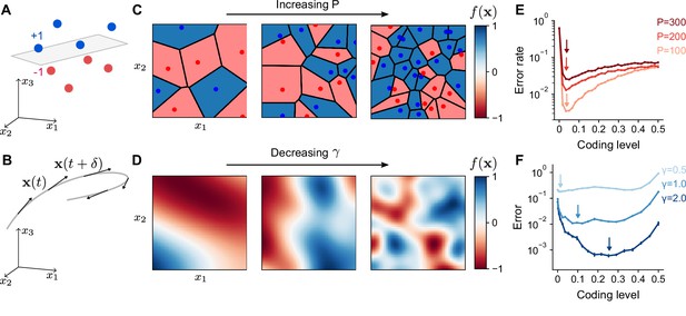
Optimal coding level depends on task.

(A) A random categorization task in which inputs are mapped to one of two categories (+1 or –1). Gray plane denotes the decision boundary of a linear classifier separating the two categories. (B) A motor control task in which inputs are the sensorimotor states $x (t)$ of an effector which change continuously along a trajectory (gray) and outputs are components of predicted future states $x (t + δ)$ . (C) Schematic of random categorization tasks with $P$ input-category associations. The value of the target function $f (x)$ (color) is a function of two task variables x₁ and x₂. (D) Schematic of tasks involving learning a continuously varying Gaussian process target parameterized by a length scale $γ$ . (E) Error rate as a function of coding level for networks trained to perform random categorization tasks similar to (C). Arrows mark estimated locations of minima. (F) Error as a function of coding level for networks trained to fit target functions sampled from Gaussian processes. Curves represent different values of the length scale parameter $γ$ . Standard error of the mean is computed across 20 realizations of network weights and sampled target functions in (E) and 200 in (F).

Figure 2—figure supplement 1

Download asset Open asset

Sparse coding levels are sufficient for random categorization tasks irrespective of number of samples, noise level, and dimension.

(A) Error as a function of coding level for networks trained to perform random categorization tasks (as in Figure 2E but with a wider range of associations $P$ ). Performance is measured for noisy instances of previously seen inputs. $D = 50$ . Dashed lines indicate the performance of a readout of the input layer. Standard error of the mean was computed across 20 realizations of network weights and tasks. (B) Same as in (A) but fixing the number of associations and varying the noise $ϵ$ which controls the deviation of test patterns from training patterns. $D = 50$ . (C) Same as in (A) but varying the input dimension $D$ . To improve performance for small $D$ , we fixed the coding level for each pattern. $P = 200, ϵ = 0.1$ For small $D$ , the curve of error rate against coding level is more flat, but low coding levels are still sufficient to saturate performance.

Figure 2—figure supplement 2

Download asset Open asset

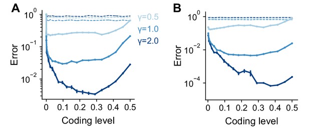
Task-dependence of optimal coding level is consistent across activation functions.

Error as a function of coding level for networks with (A) Heaviside and (B) rectified power-law (with power 2, $ϕ (u) = \max {(u, 0)}^{2}$ ) nonlinearity in the expansion layer. Networks learned Gaussian process targets. Dashed lines indicate the performance of a readout of the input layer. Standard error of the mean was computed across 10 realizations of network weights and tasks in (A) and 50 in (B). Parameters: $M = 20, 000$ , $P = 30$ , $D = 3$ .

Figure 2—figure supplement 3

Download asset Open asset

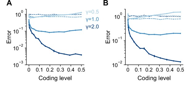
Task-dependence of optimal coding level is consistent across input dimensions.

Error as a function of coding level for networks learning Gaussian process targets with input dimension $D = 5$ (A) and $D = 7$ (B). Dashed lines indicate the performance of a readout of the input layer. Standard error of the mean was computed across 10 realizations of network weights and tasks. Parameters: $M = 20, 000$ , $P = 30$ .

Figure 2—figure supplement 4

Download asset Open asset

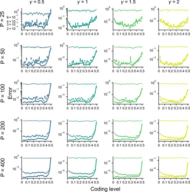
Error as a function of coding level across different values of $P$ and $γ$ .

Dots denote performance of a readout of the expansion layer in simulations. Thin lines denote performance of a readout of the input layer in simulations. Thick lines denote theory for expansion layer readout performance. Standard error of the mean was computed across 10 realizations of network weights and tasks. Parameters: $D = 3$ , $M = 20, 000$ .

Figure 3

Download asset Open asset

Effect of coding level on the expansion layer representation.

(A) Effect of activation threshold on coding level. A point on the surface of the sphere represents a neuron with effective weights $J_{i}^{e f f}$ . Blue region represents the set of neurons activated by $x$ , i.e., neurons whose input exceeds the activation threshold $θ$ (inset). Darker regions denote higher activation. (B) Effect of coding level on the overlap between population responses to different inputs. Blue and red regions represent the neurons activated by $x$ and $x^{'}$ , respectively. Overlap (purple) represents the set of neurons activated by both stimuli. High coding level leads to more active neurons and greater overlap. (C) Kernel $K (x, x^{'})$ for networks with rectified linear activation functions (Equation 1), normalized so that fully overlapping representations have an overlap of 1, plotted as a function of overlap in the space of task variables. The vertical axis corresponds to the ratio of the area of the purple region to the area of the red or blue regions in (B). Each curve corresponds to the kernel of an infinite-width network with a different coding level $f$ . (D) Dimension of the expansion layer representation as a function of coding level for a network with $M = 10, 000$ and $D = 3$ .

Figure 4 with 2 supplements

Download asset Open asset

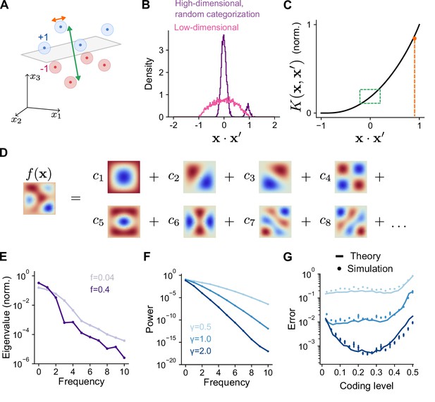
Frequency decomposition of network and target function.

(A) Geometry of high-dimensional categorization tasks where input patterns are drawn from random, noisy clusters (light regions). Performance depends on overlaps between training patterns from different clusters (green) and on overlaps between training and test patterns from the same cluster (orange). (B) Distribution of overlaps of training and test patterns in the space of task variables for a high-dimensional task ( $D = 200$ ) with random, clustered inputs as in (A) and a low-dimensional task ( $D = 5$ ) with inputs drawn uniformly on a sphere. (C) Overlaps in (A) mapped onto the kernel function. Overlaps between training patterns from different clusters are small (green). Overlaps between training and test patterns from the same cluster are large (orange). (D) Schematic illustration of basis function decomposition, for eigenfunctions on a square domain. (E) Kernel eigenvalues (normalized by the sum of eigenvalues across modes) as a function of frequency for networks with different coding levels. (F) Power $c_{α}^{2}$ as a function of frequency for Gaussian process target functions. Curves represent different values of $γ$ , the length scale of the Gaussian process. Power is averaged over 20 realizations of target functions. (G) Generalization error predicted using kernel eigenvalues (E) and target function decomposition (F) for the three target function classes shown in (F). Standard error of the mean is computed across 100 realizations of network weights and target functions.

Figure 4—figure supplement 1

Download asset Open asset

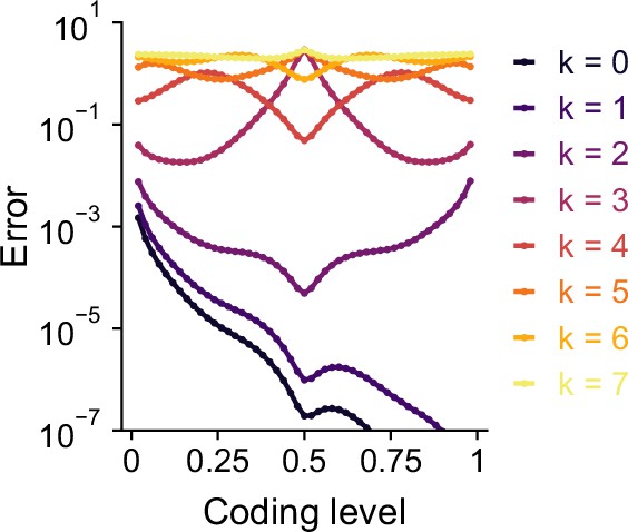
Error as a function of coding level for learning pure-frequency spherical harmonic functions.

Frequency is indexed by $k$ . Errors are calculated using analytically using Equation 4 and represent the predictions of the theory for an infinitely large expansion. Curves are symmetric around $f = 0.5$ except for $k = 0$ and $k = 1$ . Results are shown for $D = 3$ .

Figure 4—figure supplement 2

Download asset Open asset

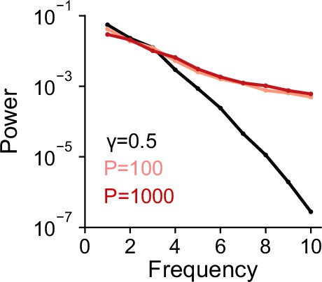
Frequency content of categorization tasks.

Power as a function of frequency for random categorization tasks (colors) and for Gaussian process task (black). Power is averaged over realizations of target functions.

Figure 5

Download asset Open asset

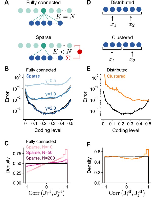
Performance of networks with sparse connectivity.

(A) Top: Fully connected network. Bottom: Sparsely connected network with in-degree $K < N$ and excitatory weights with global inhibition onto expansion layer neurons. (B) Error as a function of coding level for fully connected Gaussian weights (gray curves) and sparse excitatory weights (blue curves). Target functions are drawn from Gaussian processes with different values of length scale $γ$ as in Figure 2. (C) Distributions of synaptic weight correlations $C o r r (J_{i}^{e f f}, J_{j}^{e f f})$ , where $J_{i}^{e f f}$ is the ith row of $J^{e f f}$ , for pairs of expansion layer neurons in networks with different numbers of input layer neurons $N$ (colors) when $K = 4$ and $D = 3$ . Black distribution corresponds to fully connected networks with Gaussian weights. We note that when $D = 3$ , the distribution of correlations for random Gaussian weight vectors is uniform on $[- 1, 1]$ as shown (for higher dimensions the distribution has a peak at 0). (D) Schematic of the selectivity of input layer neurons to task variables in distributed and clustered representations. (E) Error as a function of coding level for networks with distributed (black, same as in B) and clustered (orange) representations. (F) Distributions of $C o r r (J_{i}^{e f f}, J_{j}^{e f f})$ for pairs of expansion layer neurons in networks with distributed and clustered input representations when $K = 4$ , $D = 3$ , and $N = 1, 000$ . Standard error of the mean was computed across 200 realizations in (B) and 100 in (E), orange curve.

Figure 6

Download asset Open asset

Task-independence of optimal anatomical parameters.

(A) Error as a function of in-degree $K$ for networks learning Gaussian process targets. Curves represent different values of $γ$ , the length scale of the Gaussian process. The total number of synaptic connections $S = M K$ is held constant. This constraint introduces a trade-off between having many neurons with small synaptic degree and having fewer neurons with large synaptic degree (Litwin-Kumar et al., 2017). $S = 10^{4}$ , $D = 3$ , $f = 0.3$ . (B) Error as a function of expansion ratio $M / N$ for networks learning Gaussian process targets. $D = 3$ , $N = 700$ , $f = 0.3$ . (C) Distribution of granule-cell-to-Purkinje cell weights $w$ for a network trained on nonnegative Gaussian process targets with $f = 0.3$ , $D = 3$ , $γ = 1$ . Granule-cell-to-Purkinje cell weights are constrained to be nonnegative (Brunel et al., 2004). (D) Fraction of granule-cell-to-Purkinje cell weights that are silent in networks learning nonnegative Gaussian process targets (blue) and random categorization tasks (gray).

Figure 7 with 2 supplements

Download asset Open asset

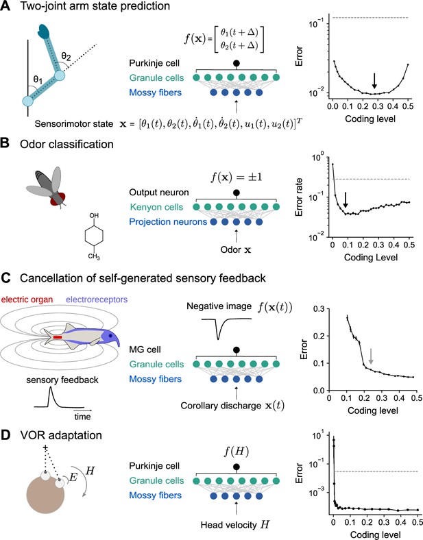
Optimal coding level across tasks and neural systems.

(A) Left: Schematic of two-joint arm. Center: Cerebellar cortex model in which sensorimotor task variables at time $t$ are used to predict hand position at time $t + δ$ . Right: Error as a function of coding level. Black arrow indicates location of optimum. Dashed line indicates performance of a readout of the input layer. (B) Left: Odor categorization task. Center: *Drosophila* mushroom body model in which odors activate olfactory projection neurons and are associated with a binary category (appetitive or aversive). Right: Error rate, similar to (A), right. (C) Left: Schematic of electrosensory system of the mormyrid electric fish, which learns a negative image to cancel the self-generated feedback from electric organ discharges sensed by electroreceptors. Center: Electrosensory lateral line lobe (ELL) model in which MG cells learn a negative image. Right: Error as a function of coding level. Gray arrow indicates location of coding level estimated from biophysical parameters (Kennedy et al., 2014). (D) Left: Schematic of the vestibulo-cular reflex (VOR). Head rotations with velocity $H$ trigger eye motion in the opposite direction with velocity $E$ . During VOR adaptation, organisms adapt to different gains ( $E / H$ ). Center: Cerebellar cortex model in which the target function is the Purkinje cell’s firing rate as a function of head velocity. Right: Error, similar to (A), right.

Figure 7—figure supplement 1

Download asset Open asset

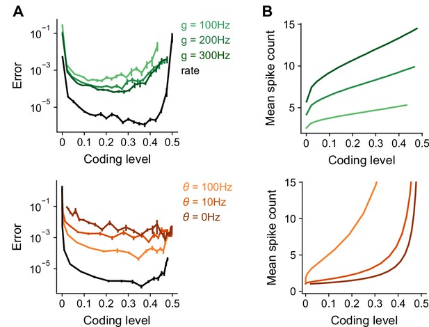
Optimal coding levels in the presence of spiking noise.

(A) Error as a function of coding level in a spiking model. The firing rate of neuron i (in Hz) is given by $h_{i}^{μ} = ϕ (g J_{i}^{e f f} x^{μ} - θ)$ , where $g$ is a gain term that adjusts the amplitude of the activity and $θ$ is the activation threshold. The spike count s_i for a neuron $i$ in response to pattern µ is sampled from a Poisson distribution: $s_{i} = P o i s (h_{i}^{μ} τ)$ represents the time window in which a Purkinje cell integrates spikes, and is set to 0.1 s. Coding level is measured as the fraction of cells with a nonzero spike count. Coding level is adjusted by tuning either the activation threshold $θ$ (top) or the gain $g$ (bottom). Black curve shows the performance of a rate model as in the main text. Standard error of the mean was computed across 10 realizations of network weights. (B) Mean spike count of active expansion layer neurons during the time window $τ$ as a function of coding level.

Figure 7—figure supplement 2

Download asset Open asset

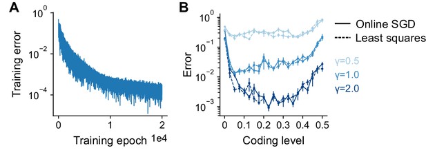
Task-dependence of optimal coding level remains consistent under an online climbing fiber-based plasticity rule.

During each epoch of training, the network is presented with all patterns in a randomized order, and the learned weights are updated with each pattern (see Methods). Networks were presented with 30 patterns and trained for 20,000 epochs, with a learning rate of $η = 0.7 / M$ . Other parameters: $D = 3, M = 10, 000$ . (A) Performance of an example network during online learning, measured as relative mean squared error across training epochs. Parameters: $f = 0.3$ , $γ = 1$ . (B) Generalization error as a function of coding level for networks trained with online learning (solid lines) or unregularized least squares (dashed lines) for Gaussian process tasks with different length scales (colors). Standard error of the mean was computed across 20 realizations.

Tables

Table 1

Summary of simulation parameters.

$M$ : number of expansion layer neurons. $N$ : number of input layer neurons. $K$ : number of connections from input layer to a single expansion layer neuron. $S$ : total number of connections from input to expansion layer. $f$ : expansion layer coding level. $D$ : number of task variables. $P$ : number of training patterns. $γ$ : Gaussian process length scale. $ϵ$ : magnitude of noise for random categorization tasks. We do not report $N$ and $K$ for simulations in which $J^{e f f}$ contains Gaussian i.i.d. elements as results do not depend on these parameters in this case.

Figure panel	Network parameters	Task parameters
Figure 2E	$M = 10, 000$	$D = 50, P = 1, 000, ϵ = 0.1$
Figures 2F, 4G and 5B (full)	$M = 200, 000$	$D = 3, P = 30$
Figure 5B and E	$M = 200, 000, N = 7, 000, K = 4$	$D = 3, P = 30$
Figure 6A	$S = M K = 10, 000, N = 100, f = 0.3$	$D = 3, P = 200$
Figure 6B	$N = 700, K = 4, f = 0.3$	$D = 3, P = 200$
Figure 6C	$M = 5, 000, f = 0.3$	$D = 3, P = 100, γ = 1$
Figure 6D	$M = 1, 000$	$D = 3, P = 50$
Figure 7A	$M = 20, 000$	$D = 6, P = 100$ ; see Methods
Figure 7B	$M = 10, 000, N = 50, K = 7$	$D = 50, P = 100, ϵ = 0.1$
Figure 7C	$M = 20, 000, N = 206, 1 \leq K \leq 3$	see Methods
Figure 7D	$M = 20, 000, N = K = 24$	$D = 1, P = 30$ ; see Methods
Figure 2—figure supplement 1	$M = 10, 000$	See Figure
Figure 2—figure supplement 2	$M = 20, 000$	$D = 3, P = 30$
Figure 2—figure supplement 3	$M = 20, 000$	$D = 3, P = 30$
Figure 2—figure supplement 4	$M = 20, 000$	$D = 3$
Figure 7—figure supplement 1	$M = 20, 000$	$D = 3, P = 200$
Figure 7—figure supplement 2	$M = 10, 000, f = 0.3$	$D = 3, P = 30, γ = 1$