Flexible coding of time or distance in hippocampal cells
- Rappaport Faculty of Medicine and Research Institute, Technion - Israel Institute of Technology, Israel
- Center for Memory and Brain, Boston University, United States
- Department of Biomedical Engineering, Boston University, United States
- Tel Aviv Sourasky Medical Center, Israel
Figures
Figure 1
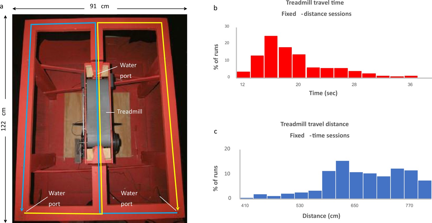
Experimental setup.
(a) The figure-eight maze with treadmill (gray belt) located in the central stem. Water ports are located near the treadmill and at the two lower corners of the maze. Blue line indicates right-to-left alternation; yellow line indicates left-to-right alternation. (b, c) Distribution of the fixed-time sessions treadmill travel times (b) and the fixed-distance sessions treadmill travel distances (c).
© 2013, Elsevier. Figure 1A is reproduced from Figure 1A from Kraus et al., 2013, with permission from Elsevier. It is not covered by the CC-BY 4.0 licence and further reproduction of this panel would need permission from the copyright holder.
Figure 2 with 1 supplement
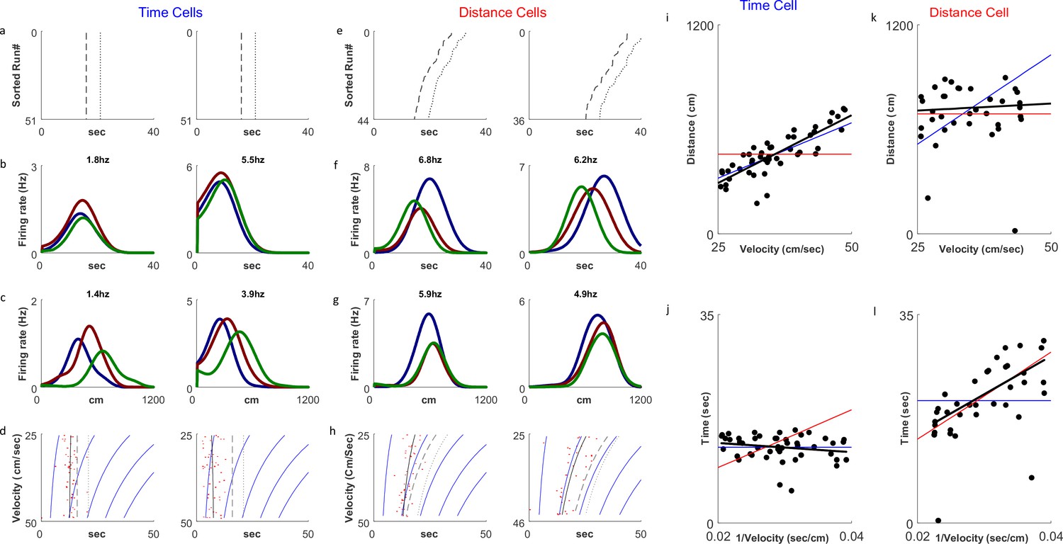
Distance and time cells coding.
(a–h) Examples of two time-coding cells (columns 1–2) and two distance-coding cells (columns 3–4). Row a depicts neural firing as a function of the distance the animal traveled, sorted by the runs’ velocities. The colors represent three velocity groups for which the tuning curves, by time or distance, are presented in rows b and c, respectively. Row d shows the onsets of each run (red dots) and their linear fit (black curve) to the relation for the time cells and for the distance cells. The dashed curve represents the end-of-run time, and the dotted curve represents the end of the analyzed period (treadmill stop time, plus 5 seconds). The blue curves are equi-distance points in time. A black curve (the linear fit) which is parallel to the equi-distance curves demonstrates a cell with strong distance coding. (i–l) Examples of the analysis of time (i, j) and distance (k, l) encoding cells. Top row plots depict distance vs. velocity and bottom row plots depict onset vs. 1/velocity. Red line represents an ideal Distance Cell, based on the average distance traveled until the onset time. Blue line represents an ideal Time Cell, based on the average time of the onset and the black line is the linear fit. The closer the slope of the black line is to that of the red line, relative to slope of the blue line, the more the cell encodes distance-encoding, while if the slope is closer to the slope of the blue line, the is more it is time-encoding.
Figure 2—figure supplement 1
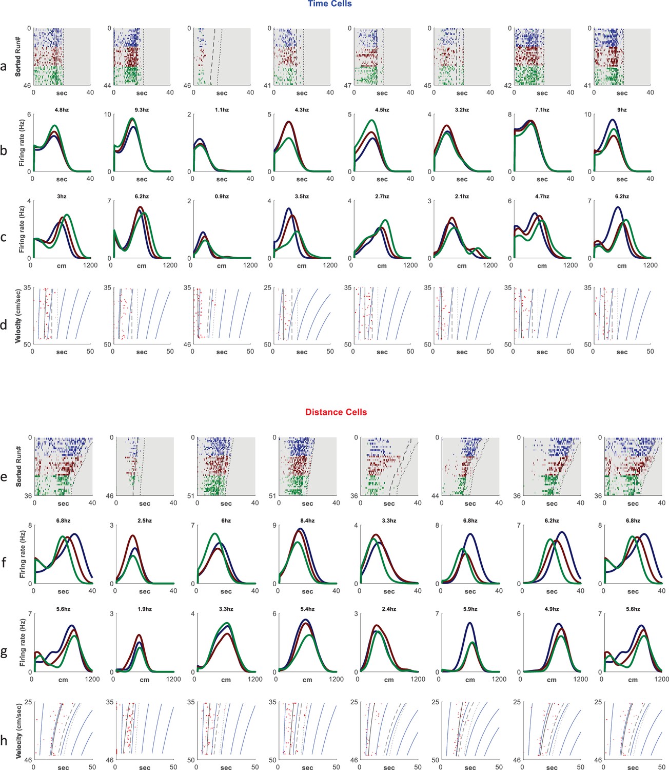
Additional examples of cells showing time coding (a–d) and distance encoding (e–h).
Rows a,e depict neural firing as a function of time, sorted by the run’s velocities. The colors represent three velocity groups for which the tuning curves, either by time or distance, are presented in rows b, f and c, g respectively. Rows d, h show the onsets of each run (red dots) and their linear fit (black curve) based on the relation for the time cells and for the distance cells. Dashed curves represent treadmill stop time and dotted curves represent end of period analyzed (treadmill stop time plus 5 s). Blue curves are equi-distance points in time while dashed curve represents end of run time. The more a linear fit curve is vertical the more significant is the time coding of that cell.
Figure 3 with 3 supplements
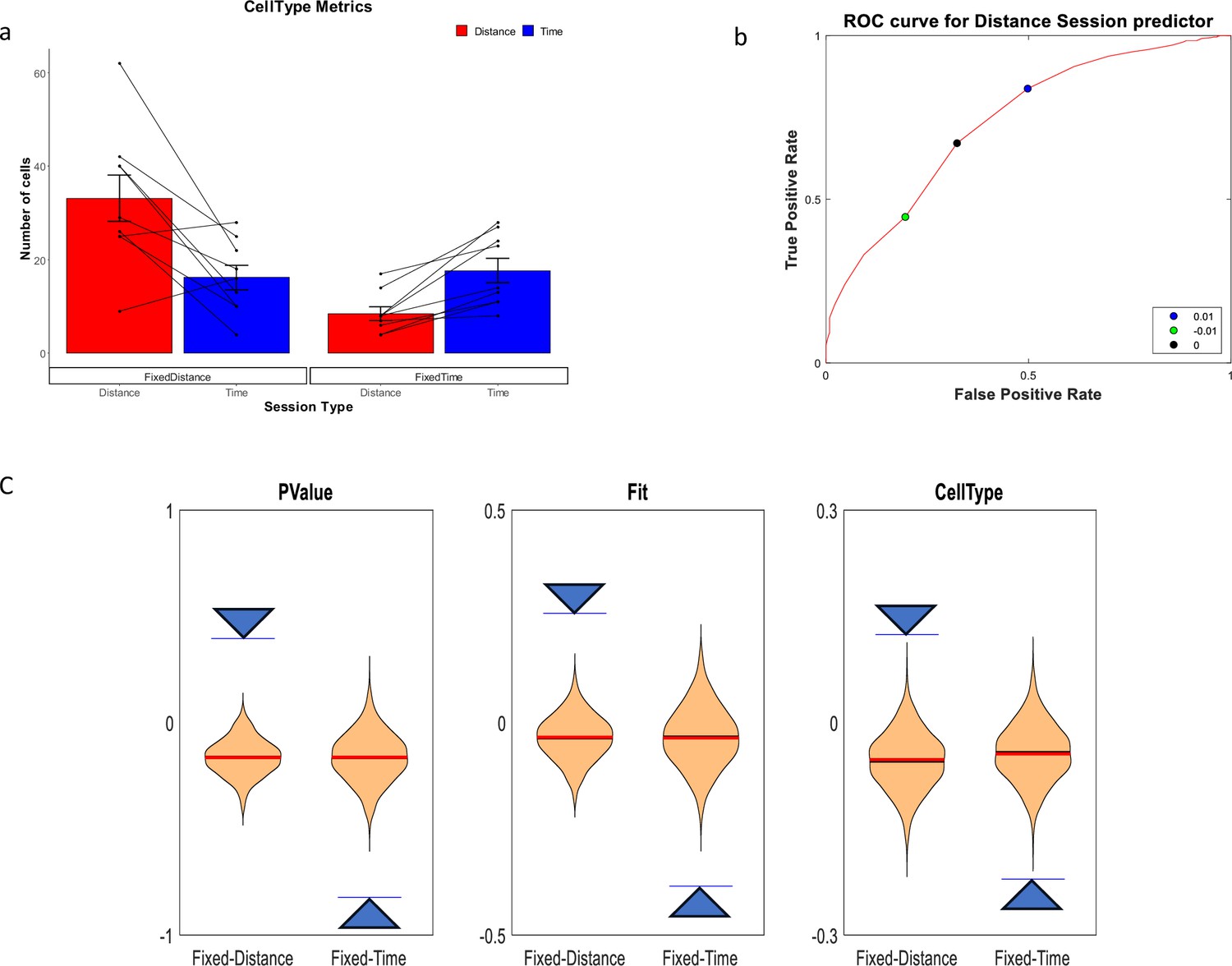
Distance and Time Cells classification.
(a) Cells type classified by the CellType metric, averaged over all animals and trials, for fixed-distance and fixed-time experiments (n=18 experiments, mean ± SEM) p<<0.001 by Pearson's chi-squared test using two categories. Diagonal lines represent individual animals. (b) ROC curve (red) showing that the chosen discriminating threshold of 0 (black point) is optimal. The True Positive Rate (TPR) is the percentage of cells classified as distance cells on the fixed-distance session, while the False Positive Rate (FPR) is the percentage of cells classified as distance cells on the fixed-time sessions. (c) Shuffling distribution of the three metrics: CellType, FIT and P-Value. The type of experiment, either fixed-time or fixed-distance, was randomized 1000 times for each of the sessions. All experiments were truncated to 16 s in order to prevent biases. The vertical axis is the Time-Distance balance index (TDI), defined as (#DistanceCells-#TimeCells)/(#DistanceCells + TimeCells) and is between 0 and 1 if there are more distance cells than time cells and between –1 and 0 if there are more time cells than distance cells. The arrows are indicating the actual results which are significant compared to the shuffle distribution.
Figure 3—figure supplement 1
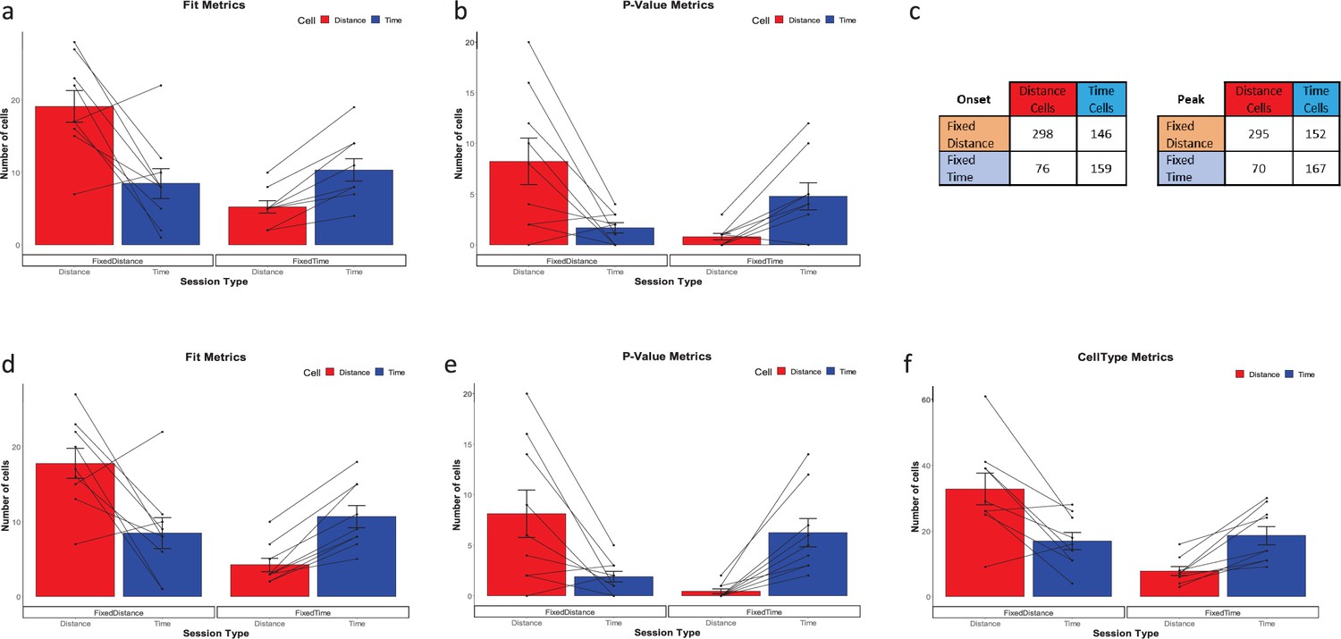
Additional metrics.
Cells type classified by the FIT metric (a) and p-Value metric (b), averaged over all animals and trials, for fixed distance and fixed time experiments (n=18 experiments, mean ± SEM) p<<0.001 by Pearson's chi-squared test using two categories. The whiskers show the SEM and the points and the lines connecting the points represent individual animal results. (c) Comparison of onset vs peak analysis cells count in each category (d–f) CellType, Fit and p-Value metrics results for a peak-based analysis.
Figure 3—figure supplement 2
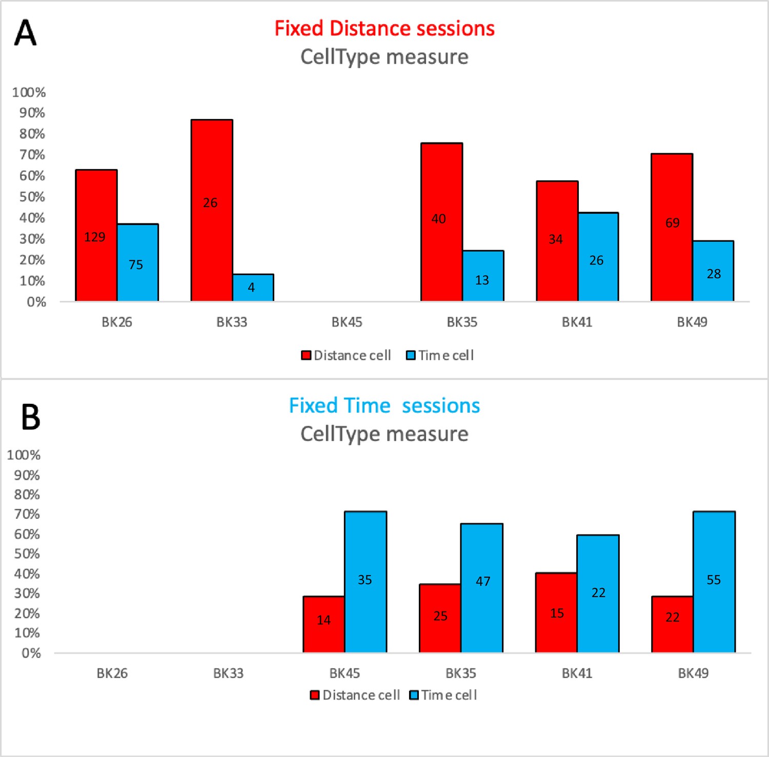
The distribution of Time and Place cells, per animal, at various metrics, for Time and Distance sessions.
Animals BK26 (n=3 experiments) and BK33 (n=1 experiment) participated only in distance sessions, while BK45 (n=3 experiments) participated only in a time session, and BK35 (n=3 experiments), BK41 (n=4 experiments) and BK49 (n=4 experiments) participated in both types of sessions. All distributions show a significant dependency on the session type (χ2(1)>12, p<<0.001 for BK35,BK49,BK45,BK33 and χ2(1)=5.7, p<0.02 for BK26 by Pearson's chi-squared test using two categories.), except for animal BK41 (χ2(1)=2.38, p=0.12). The bars represent the percentage of the respective cell type from the entire population of cells in the respective session. The numbers inside the bars represent the number of cells. For the single session animals, the reference distribution used for the χ2 test was taken from the entire population distribution (55% Distance Cells and 45% Time Cells).
Figure 3—figure supplement 3
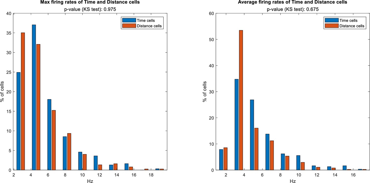
Distribution of max and average firing rates for Time and Distance cells.
Total 304 time cells and 374 distance cells evaluated. The time cells and distance cells distributions are similar (p=0.975, Kolmogorov-Smirnov test for the max firing rate, p=0.675 for the average firing rate).
Additional files
Download links
A two-part list of links to download the article, or parts of the article, in various formats.
Downloads (link to download the article as PDF)
Open citations (links to open the citations from this article in various online reference manager services)
Cite this article (links to download the citations from this article in formats compatible with various reference manager tools)
Flexible coding of time or distance in hippocampal cells
eLife 12:e83930.
https://doi.org/10.7554/eLife.83930


