Bayesian analysis of phase data in EEG and MEG
- Faculty of Engineering, University of Bristol, United Kingdom
- School of Computing, Engineering & Intelligent Systems, Ulster University, United Kingdom
Figures
Figure 1

The syntactic target for the experiment.
In the adjective–noun (AN) stimulus, there are noun phrases at the phrase rate, 1.5625 Hz; this structure is absent in the adjective–verb (AV) stimulus because AV pairs do not form a phrase. 3.125 Hz corresponds to the syllable rate in this experiment.
Figure 2
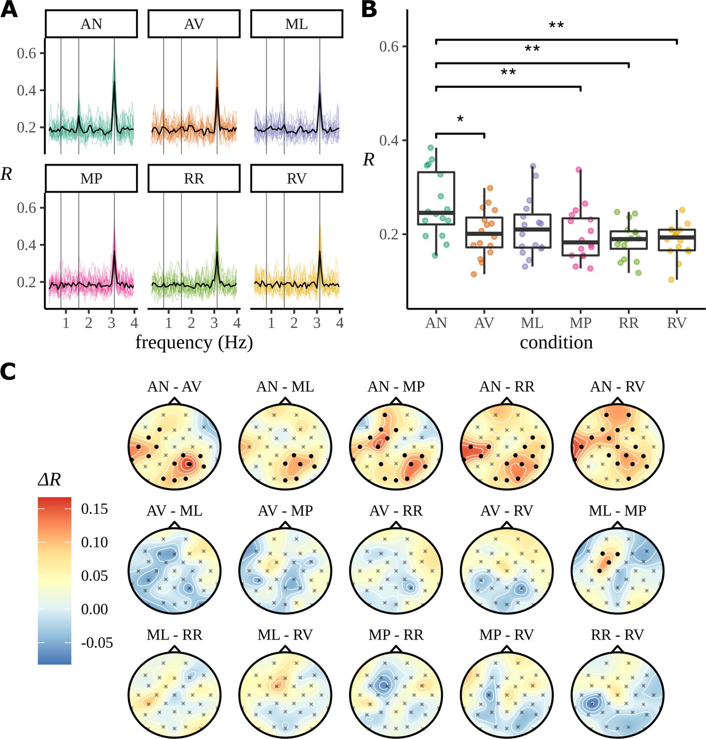
Summarising the inter-trial phase coherence (ITPC) for different conditions.
(A) Coloured lines show the ITPC for each participant after averaging over electrodes and is traced across all frequencies. The mean trace, calculated by averaging over all participant traces, is overlaid in black. Vertical lines mark the sentence, phrase, and syllable frequencies as increasing frequencies, respectively. (B) Statistical significance was observed with an uncorrected paired two-sided Wilcoxon signed-rank test (∗0.05, ∗∗0.01). (C) ITPC differences for each condition pair calculated at the phrase frequency and interpolated across the skull. Filled circular points mark clusters of electrodes that were discovered to be significantly different (p<0.05) by the cluster-based permutation test.
Figure 3

Pseudowords and position-controlled syllables.
All six pseudowords used in the experiment are numbered. Groups of position-controlled syllables have been coloured.
Figure 4
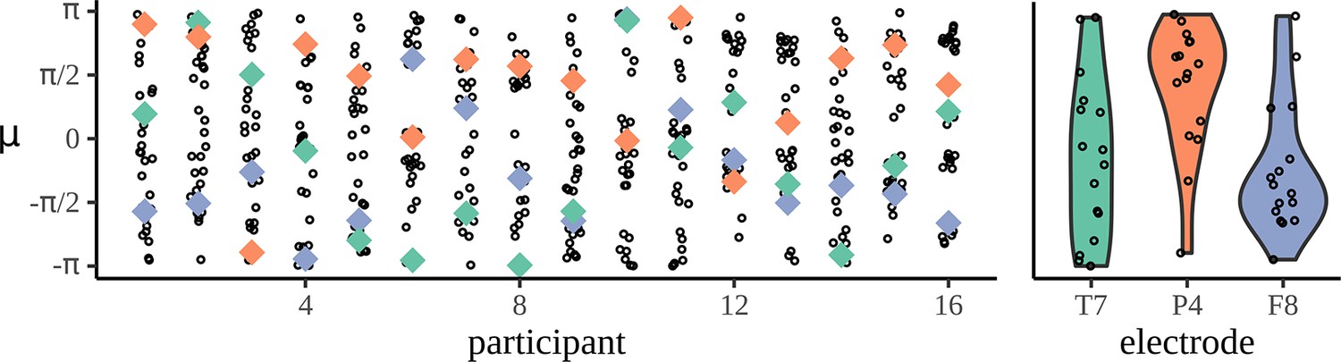
Mean phases are uniform across participants.
The left-hand panel shows the distribution of phases across electrodes for each participant: each column corresponds to one participant and each dot marks the mean phase µ for each of the 32 electrodes calculated at the phrase frequency for the adjective–noun (AN) grammatical condition. To show how a given electrode varies across participant, three example electrodes are marked, T7 in green, P4 in orange, and F8 in purple. The right-hand panel shows the distribution of mean phases, µ, across participants.
Figure 5
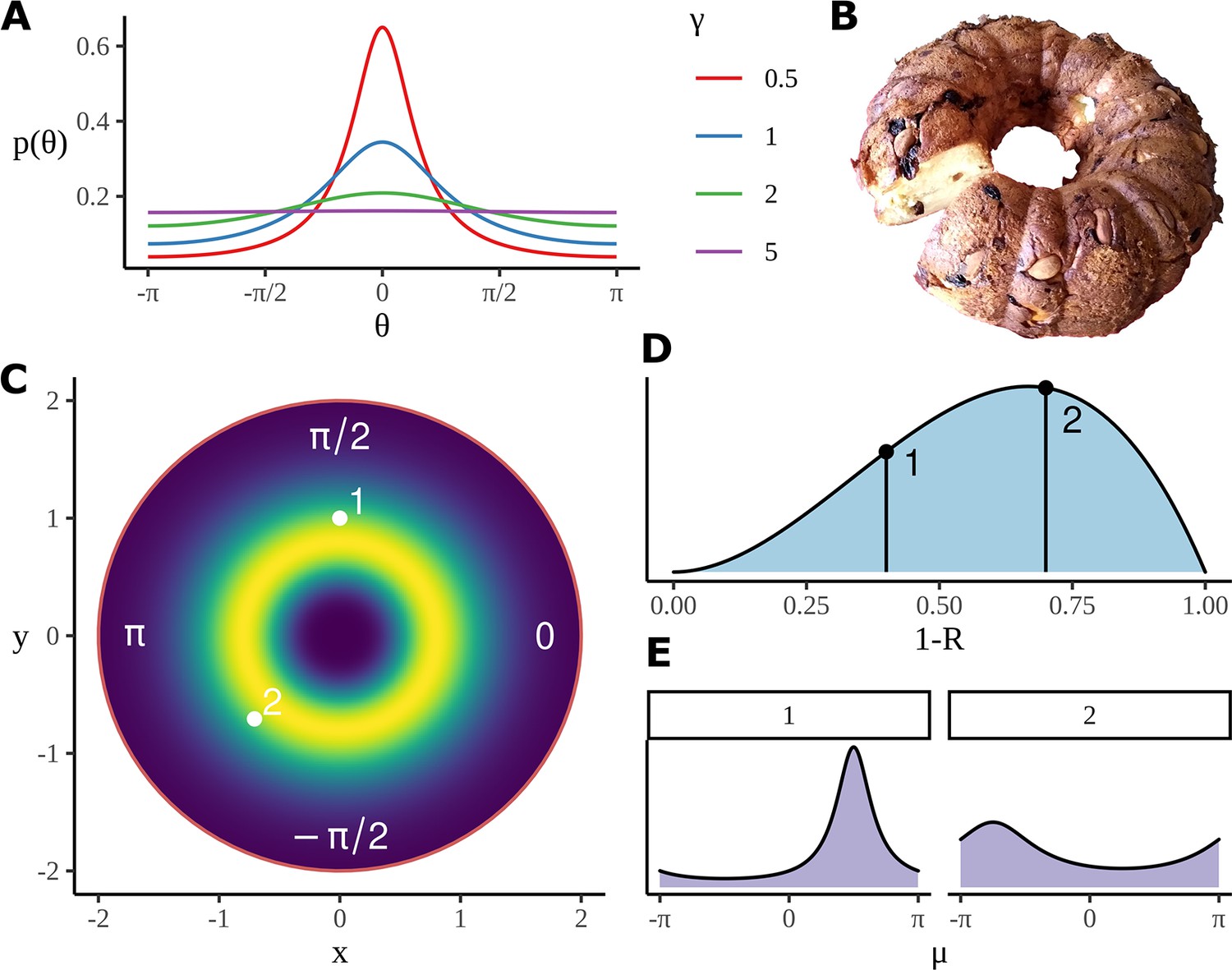
Model construction and geometry.
(A) Example wrapped Cauchy density functions for different values of the scale parameter. (B) The Bundt distribution has a shape reminiscent of a cake made in a Bundt tin. (C) The mean phase is sampled from an axially symmetric prior distribution with a soft constraint on the radius. Highlighted pairs give the location of example points; these points correspond to the mean angle for a wrapped Cauchy distribution using . (D) An example distribution for which determines the parameter in the wrapped Cauchy distribution. is related to other parameters such a condition and participant number through a logistic regression, as in Equation 19, the priors for the slopes in the regression are used to produce the distribution shown here; as before, two example points are chosen, each will correspond to a different value of in the corresponding wrapped Cauchy distribution. (E) Example wrapped Cauchy distributions are plotted in correspondence with the numbered prior proposals in (C) and (D).
Figure 6

Posterior distributions.
(A) The traces show point estimates of the mean resultant length calculated across all 58 frequencies using the optimisation procedure. (B) The marginal posterior distributions for each transformed condition effect are shown with a violin plot. Posteriors over condition differences are given directly above, the colour of which represents the condition against which the comparison is made. For example, the green interval above the adjective–verb (AV) condition describes the posterior difference . Posterior differences and marginal intervals are all given as 90% highest density intervals (HDIs) marked with posterior medians. (C) Posterior medians are interpolated across the skull for all condition comparisons. Filled circle shows those electrodes where zero was not present in the 95% HDI for the marginal posteriors over the quantity in Equation 22.
Figure 7

Participant attentiveness and localised electrode effects.
(A) The intervals show participant effects for the grammatical adjective–noun (AN) condition given as 50/90% highest density intervals (HDIs) and posterior medians. (B) The posterior distributions over the standard deviation of participant slopes for each condition. Outer vertical lines mark the 90% posterior HDIs, inner lines mark the posterior median. (C) The skull plot from Figure 6C for the AN–AV difference with electrode names marked. (D) Posterior distributions over electrode differences for those positions on the skull where the grammatical condition shows a higher coherence of phases at the average participant in (C). Intervals give 50/90% HDIs and the posterior medians. AV, adjective–verb.
Figure 8
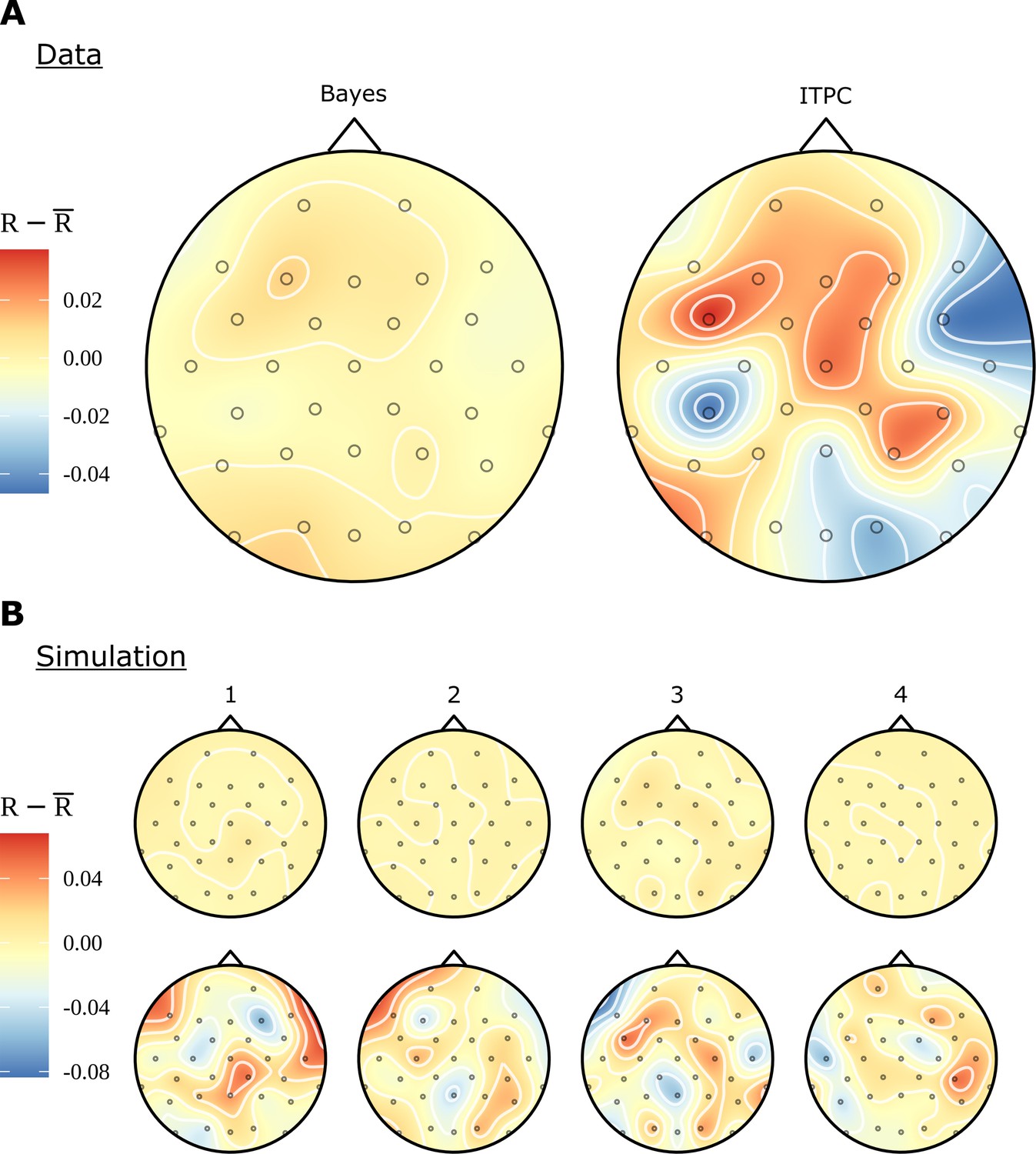
Comparison of electrode effects for no signal.
(A) Topographic headcaps for the phrase data using the random words condition (RR). When calculating phase coherence using the inter-trial phase coherence (ITPC) for this condition, there is an apparent high but misleading variation in electrodes across the skull. This does not manifest in the Bayesian result due to regularisation of the electrode effects. (B) Data was simulated from the generative Bayesian model four times with electrode effects set to zero to provide a known ground truth. Plots can be thought of as results from four separate experiments. On this simulated data, the ITPC shows variation similar to (A); the Bayesian results are consistent with the ground truth. The ITPC has an upward bias, so in all figures the mean was subtracted for ease of comparison.
Figure 9
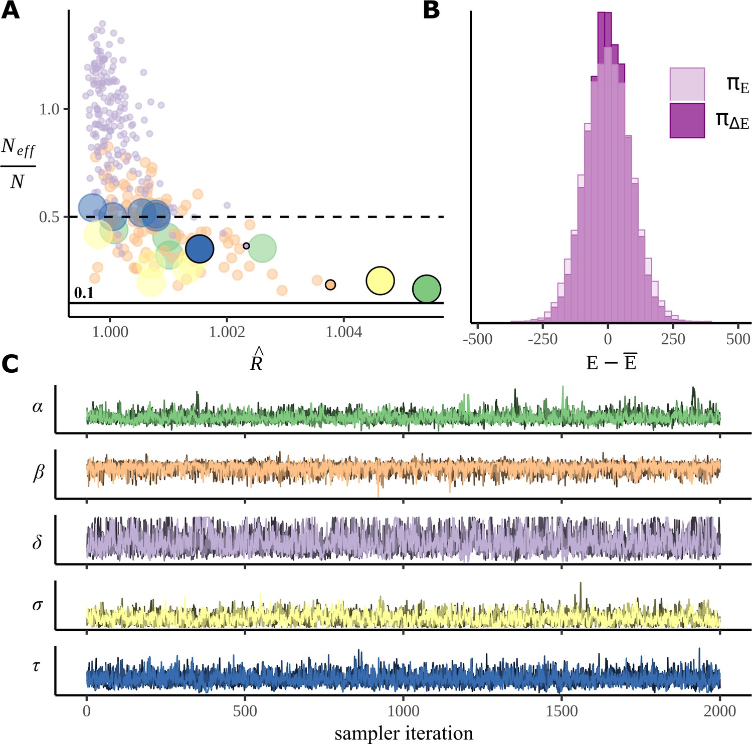
Sampler performance and diagnostics.
(A) The performance of the sampler is illustrated by plotting (R-hat) against the ratio of the effective number of samples for each parameter in the model. Points represent individual model parameters grouped by colour with a different colour for each parameter type. For convenience, the dot sizes are scaled, so the more numerous parameters have smaller dots, the less numerous, fewer, so, for example, with only six examples, is large. (B) A histogram comparing the marginal energy distribution , and the transitional energy distribution of the Hamiltonian. (C) Post-warmup trace plots. All four chains for the poorest performing parameter within each parameter group are overlaid. Corresponding points in (A) are marked with a black border and zero transparency.
Figure 10
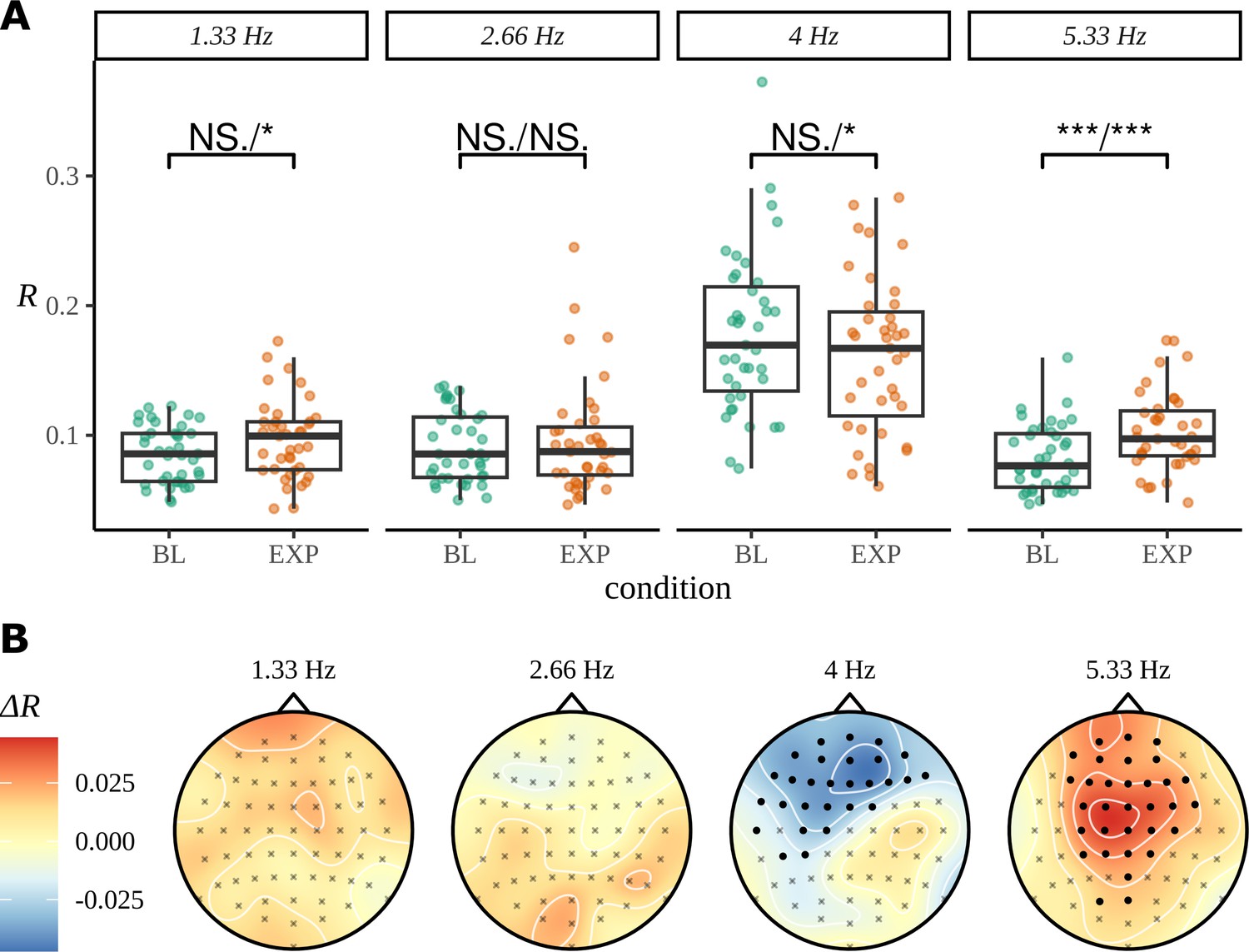
Inter-trial phase coherence (ITPC) analysis.
(A) ITPC averages across all trials and electrodes for each of the 39 participants. We replicate the statistical procedure as stated in Pinto et al., 2022 of paired one-sided test of a greater ITPC mean of experimental condition (EXP) at the pseudoword rate (1.33 Hz) and its first and second harmonics (2.66 Hz, 5.33 Hz). A one-sided test for a larger ITPC value of the baseline condition (BL) at the syllable rate is also performed. Significance values on the specified test results of an uncorrected paired Wilcoxon signed-rank test (left) and an uncorrected paired t-test (right). (B) Statistically significant clusters of electrodes were found using a cluster-based permutation test between these two conditions at 4 Hz and 5.33 Hz.
Figure 11
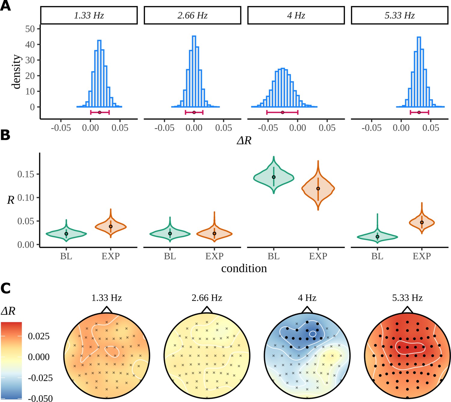
Bayes analysis for the statistical learning data set.
(A) Posterior distributions over the condition difference are shown for all frequencies of interest. In each case, the full posterior is given by the histogram and is annotated by its 90% highest density interval (HDI) and posterior median. (B) Marginal posterior distributions over the mean resultant length for each condition and frequency of interest. (C) Posterior means for the difference at each of the 64 electrodes are interpolated across the skull. Filled circles label those electrodes where zero was not contained by the 95% HDI calculated from the quantity in Equation 22.
Figure 12
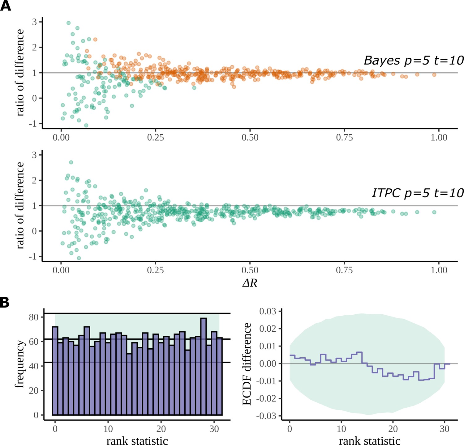
Simulation study.
(A) The Bayesian model has a higher true detection rate for lower participant numbers. The bias of the estimate is also greatly reduced by the Bayesian model. As the real difference increases along the x axis, the variation in model estimates reduces in both methods; however, the distribution of these points around is much more symmetric for the Bayesian model; this result highlights its bias reduction. The y axis has been restricted to help highlight the behaviour of interest. (B) Simulation-based calibration for the same participant and trial numbers where the rank of is analysed. There is no evidence to suggest a tendency of the Bayesian model to overestimate or underestimate the difference.
Figure 13
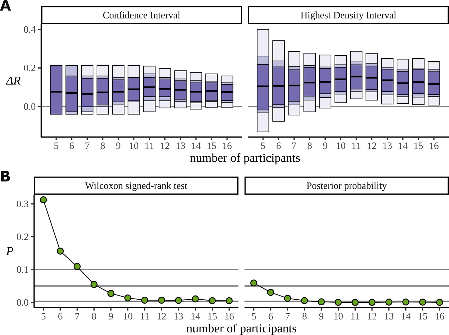
Efficiency of the frequentist and Bayesian approaches for participant number.
(A) Confidence intervals arising from a two-sided paired Wilcoxon signed-rank (left), alongside Bayesian highest density intervals (right), calculated for the condition difference AN-RR in the phrase dataset. The intervals give widths 90/95/99.7% for each method respectively. (B) The p-value arising from the same significance test (left) compared with the probability of observing a value less than zero by the posterior distribution (right).
Figure 14
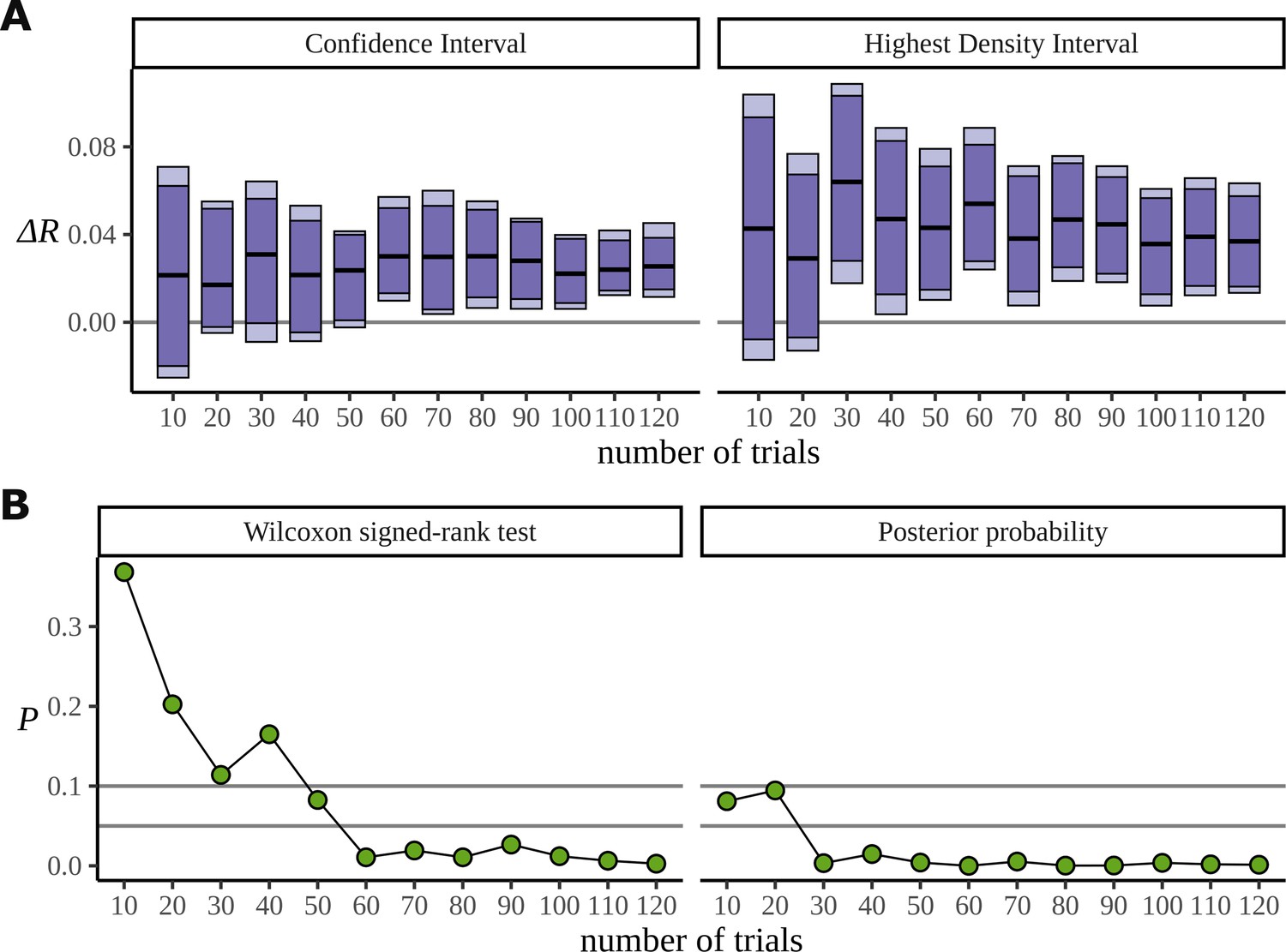
Efficiency of the frequentist and Bayesian approaches for trial number.
(A) Confidence intervals arising from a two-sided paired Wilcoxon signed-rank (left), alongside Bayesian highest density intervals (HDIs) (right), calculated for the condition difference EXP-BL in the statistical learning dataset. The intervals are given for confidence levels of 90 and 95%. On the right are the HDIs for the same levels. (B) The p-value arising from the significance test (left) compared with the probability of observing a value less than zero by the posterior distribution (right).
Appendix 5—figure 1

True discovery rates.
A summary of more participant and trial numbers of the plots shown in Figure 12A. For five participants, a doubling of the number of trials still provides insufficient information for the inter-trial phase coherence (ITPC) and resulting significance test to conclude that a difference exists in any simulation. Bars show the 95% confidence intervals on this measure estimated through bootstrap.
Appendix 6—figure 1

False discovery rates.
The frequentist approach to inter-trial phase coherence (ITPC) differences using a paired Wilcoxon signed-rank test has a type 1 error that increases with both participant and trial number. Bars show the 95% confidence intervals on this measure estimated through bootstrap.
Appendix 8—figure 1
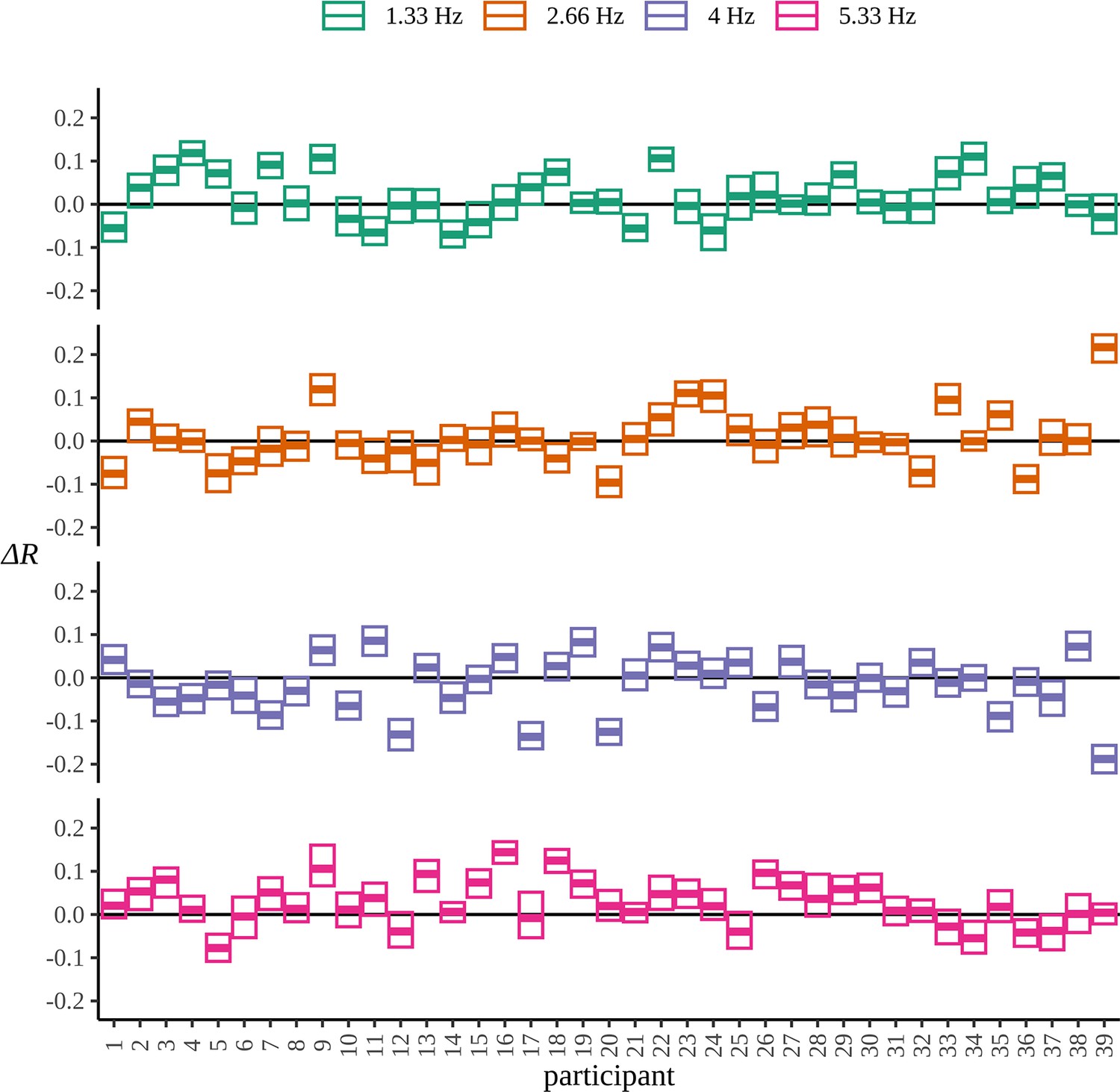
Participant posteriors.
Highest density intervals containing 99% of the posterior probability for each participant and frequency over the difference in mean resultant length EXP-BL.
Appendix 9—figure 1
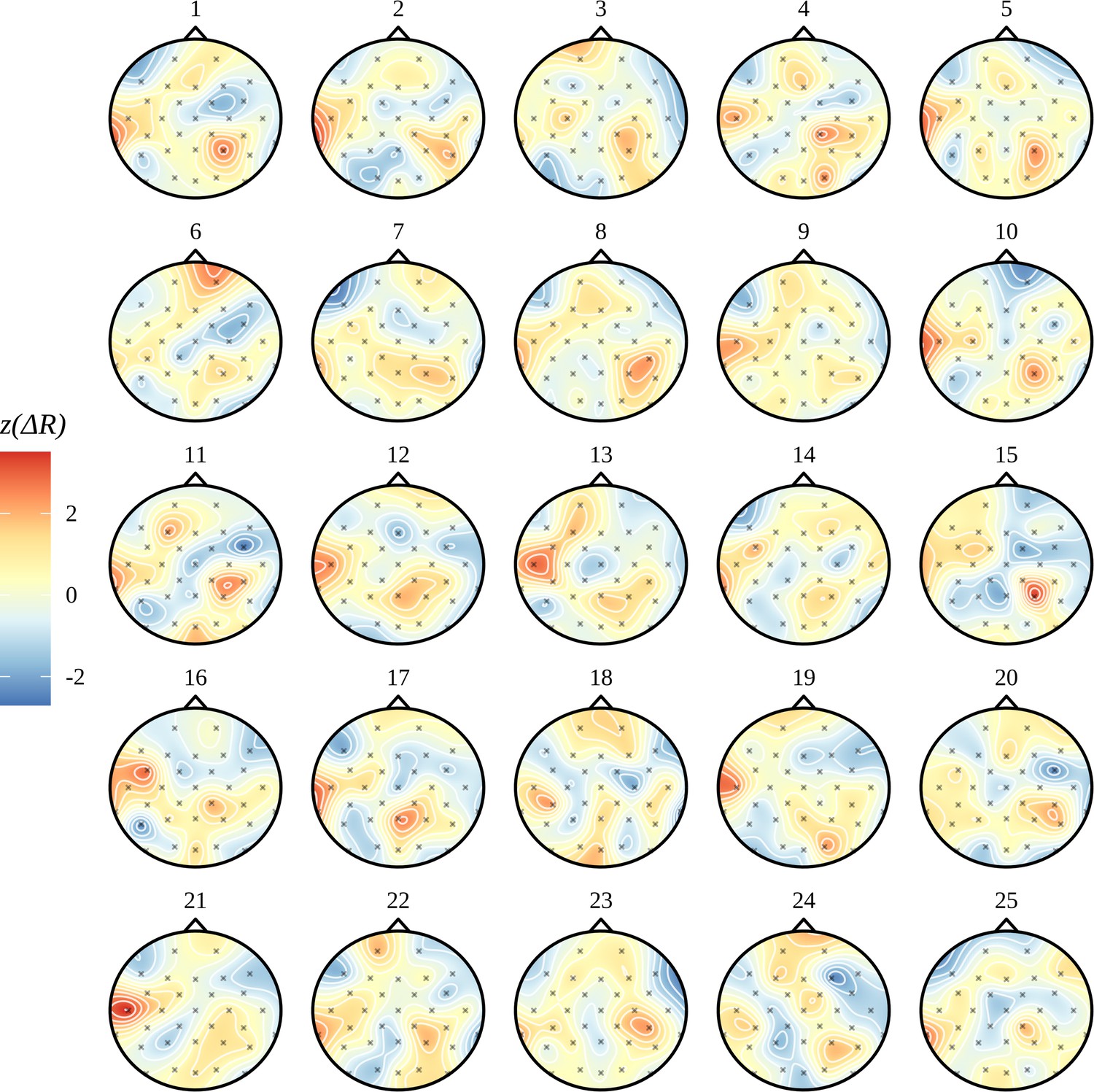
Joint headcap posterior.
Here we visualise uncertainty in the posterior over the difference AN-AV and how it captures a range of plausible activity patterns. As expected, samples demonstrate variation about the mean shown in Figure 6B of a right parietal and left temporal activation. AN: adjective–noun; AV: adjective–verb.
Tables
Table 1
Summary of posterior values for the statistical learning dataset.
All values are rounded to three decimal places. The difference shown is EXP-BL. HDI: highest density interval.
| Frequency (Hz) | Mean | Median | SD | 90% HDI |
|---|---|---|---|---|
| 1.33 | 0.016 | 0.016 | 0.010 | [0.001, 0.032] |
| 2.66 | 0.000 | 0.000 | 0.009 | [–0.014, 0.015] |
| 4 | –0.025 | –0.025 | 0.016 | [–0.052, 0.000] |
| 5.33 | 0.030 | 0.030 | 0.009 | [0.016, 0.046] |
Appendix 3—table 1
Table of conditions for the phrase dataset.
| Condition | Description | Example |
|---|---|---|
| AN | Adjective–noun pairs | …old rat sad man… |
| AV | Adjective–verb pairs | …rough give ill tell… |
| ML | Adjective–pronoun verb–preposition | …old this ask in… |
| MP | Mixed grammatical phrases | …not full more green… |
| RV | Random words with every fourth a verb | …his old from think… |
| RR | Random words | …large out fetch her… |
Additional files
Download links
A two-part list of links to download the article, or parts of the article, in various formats.
Downloads (link to download the article as PDF)
Open citations (links to open the citations from this article in various online reference manager services)
Cite this article (links to download the citations from this article in formats compatible with various reference manager tools)
Bayesian analysis of phase data in EEG and MEG
eLife 12:e84602.
https://doi.org/10.7554/eLife.84602


