A comprehensive model of Drosophila epithelium reveals the role of embryo geometry and cell topology in mechanical responses
- Department of Biophysics, University of Texas Southwestern Medical Center, United States
- Department of Chemical and Biomolecular Engineering, University of California, Berkeley, United States
- Chemical Sciences Division, Lawrence Berkeley National Laboratory, United States
- Department of Bioinformatics, University of Texas Southwestern Medical Center, United States
- Department of Material Science and Engineering, University of Texas at Arlington, United States
Figures
Figure 1 with 1 supplement
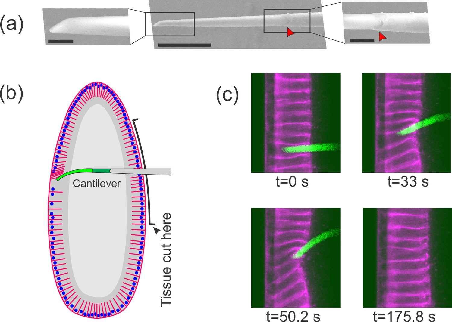
Flexible cantilevers can be used as a probe for tissue properties.
(a) Scanning electron microscopy (SEM) image of a typical cantilever. Scale bars are 5, 30, and 10 μm respectively from left to right. Left and right panels are zoomed-in views of boxed regions in the central panel. The junction where the glass pipette ends and the flexible, polymer-only portion begins is indicated with a red arrowhead. Technical details of cantilever microfabrication are shown in Figure 1—figure supplement 1. (b) Schematic of the pulling experiment. The embryo is cut along the ventral side and the cantilever is inserted through the cut. At the relevant developmental stage, cells have a ‘hole’ on their basal side such that they are open to the interior. The flexible tip of the cantilever is inserted into a cell through the basal hole and translated so as to deform the cellular layer. (c) A sample measurement. To visualize cellular deformations arising from the applied force, cellular membranes are stained with a bright fluorescent dye (CellMask Deep Red) injected into the perivitelline space prior to measurement. The cantilever (green) is inserted into one of the cells (magenta) and is pulled upward. The resulting deflection of the cantilever as well as the deformation of the cellular layer is readily visible and quantifiable.
Figure 1—figure supplement 1
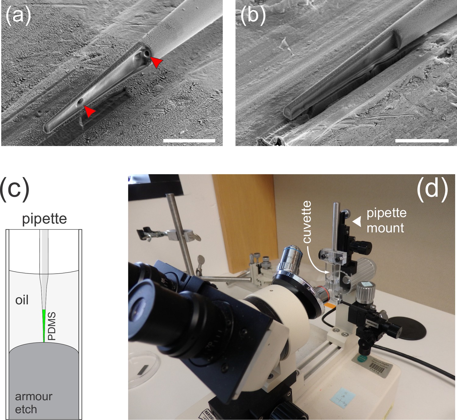
Details of cantilever microfabrication.
(a–b) Longitudinal sections through the tip of a polymer-filled glass pipette made using cryo focused ion beam milling. The sample in (a) was microfabricated by back-filling a glass pipette with polydimethylsiloxane (PDMS)-boron-dipyrromethene (BODIPY) mixture, whereas the sample in (b) was filled through the front by capillary action. The sample in (a) contains sub-micron-sized bubbles trapped in the polymer (red arrowheads). Feeding in the polymer through the tip eliminates bubbles, so this was the final protocol we adopted. (c) Schematic of the setup used to microfabricate cantilevers. BODIPY-infused PDMS is loaded into a pulled glass pipette. The pipette is then immersed into a dilute solution of hydrofluoric acid (Armour etch, https://www.armourproducts.com/) to etch away the glass from the 60-µm-long portion of the tip. (d) A cuvette with the etching solution mounted on a retrofitted Microforge instrument. The pipette can be immersed into the etching solution using a micromanipulator and is simultaneously observed through a horizontally mounted microscope.
Figure 2 with 1 supplement
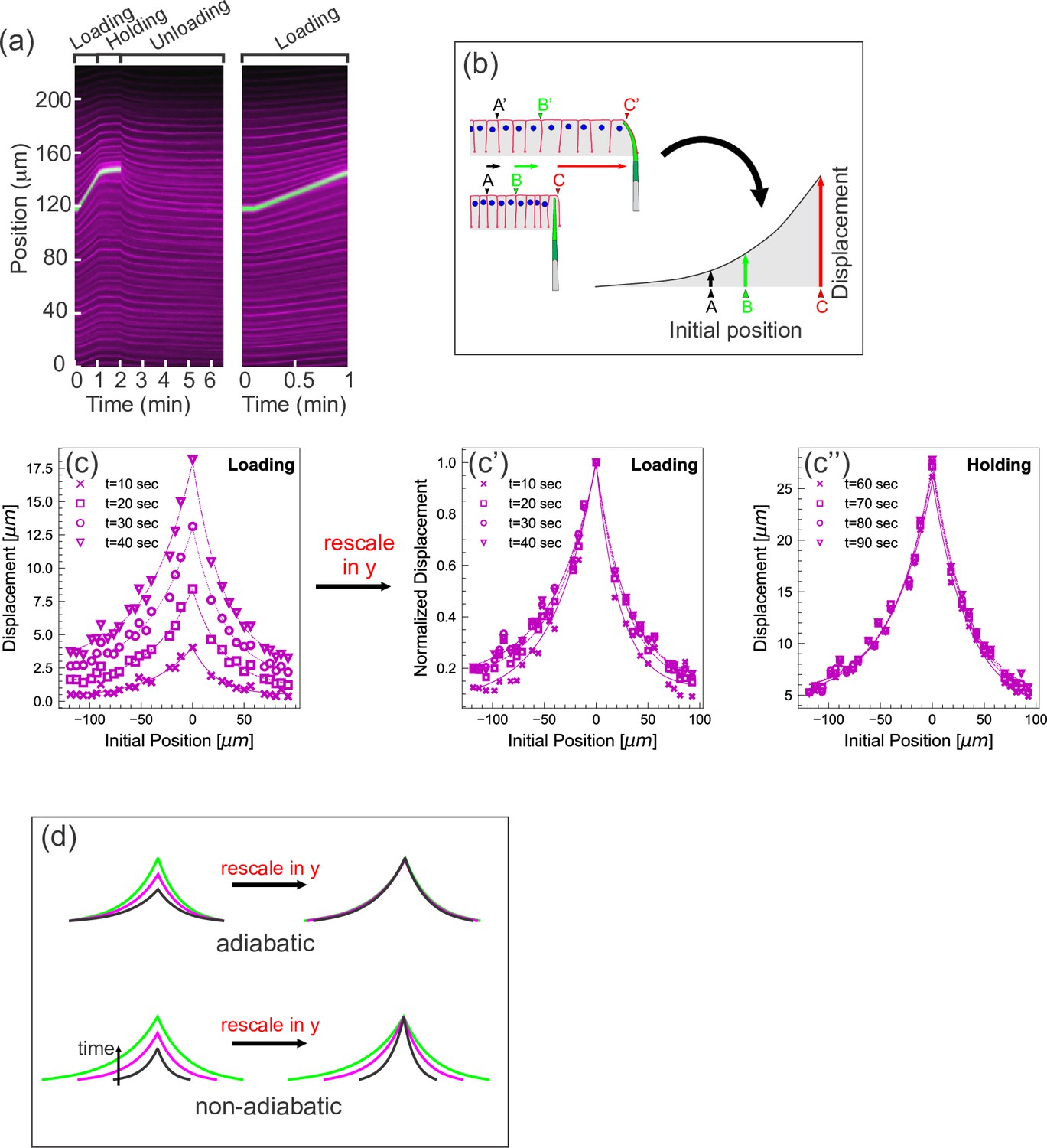
Quantifying tissue deformation during cantilever-based experiments.
(a) Left kymograph corresponds to a complete loading-unloading cycle. Right panel is a zoomed-in portion of the same kymograph showing the loading phase only. Green streak reflects signal from the cantilever; magenta streaks reflect signal from the cell membranes. During the loading phase, when the cantilever base is being translated 0.5 µm/s, the green cantilever trace appears as a straight line, since the deflection of the soft cantilever tip is small relative to the translation of the base. (b) Schematic illustrating how a tissue deformation profile is constructed based on the data in a kymograph. (c) Tissue deformation profiles at several time points during the loading phase, extracted from the kymograph in (a). Deformation profiles were highly reproducible between individual experiment, shown in Figure 2—figure supplement 1. (c') Same as (c), with the curves linearly re-scaled along the y-axis so as to have the same maximum at zero. (c’’) Tissue deformation profile at several time points during the holding phase, also extracted from the kymograph in (a). (d) Cartoon showing the expected outcomes of linearly re-scaling tissue deformation profiles for force loading under two mechanical regimes. In adiabatic regimes, curves from different time points should appear roughly the same when linearly re-scaled along the y-axis only. In non-adiabatic regimes, linearly re-scaling along the y-axis only is insufficient to generate similar curves.
Figure 2—figure supplement 1
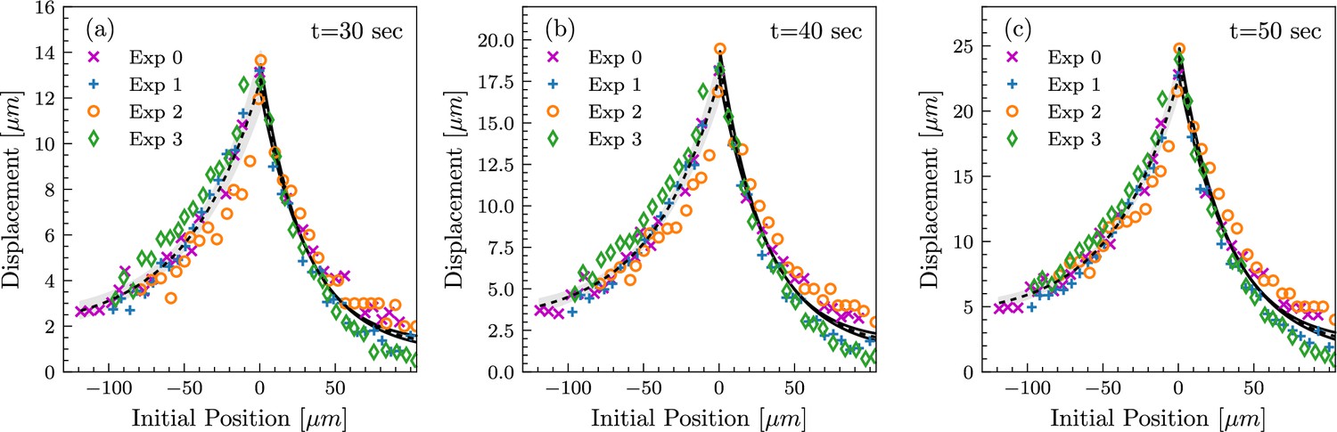
Tissue deformation profiles are highly reproducible between measurements.
Tissue deformation curves from four independent experiments, shown at time points t=30 sec, t=40 sec, and t=50 sec (a, b, and c, respectively), in the loading phase. Analogous to the measurements in Figure 2c. In all four experiments, the length of the lateral membranes at the beginning of pulling was between 15 and 20 µm, corresponding to the mid-cellularization stage.
Figure 3 with 1 supplement
Quantifying applied force during cantilever-based experiments.
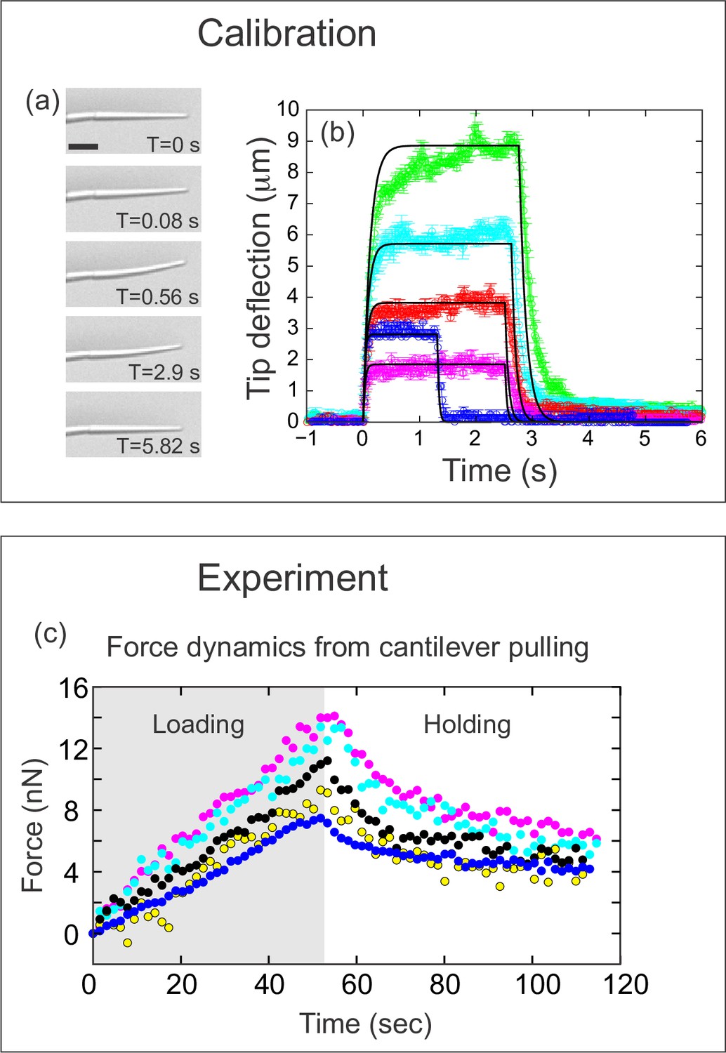
(a) Images from force calibration experiment. A cantilever was dragged through a fluid of known viscosity (Tween 20). Different snapshots show the profile of the cantilever at different times. Scale bar: 20 μm. (b) Quantification from force calibration experiment. Cantilever tip deflection as a function of time for five different cantilevers being dragged through Tween 20. The flexible tip quickly reaches a steady-state degree of deflection when dragged at a fixed velocity, and thus is under the influence of a constant force. The approach used to calculate the elastic modulus of the boron-dipyrromethene (BODIPY)-infused polydimethylsiloxane (PDMS) from these data is given in the Materials and methods section. Additional approaches are described in Figure 3—figure supplement 1. The differences in magnitude of force deflection seen here are due to the different dimensions of each cantilever. Cantilevers used for in vivo experiments were individually calibrated taking the dimensions of the particular cantilever into account. (c) Force on cantilever as a function of time in five different in vivo pulling experiments. Force was calculated from cantilever deflection as described in Materials and methods. Only the loading (gray background) and holding (white background) phases of the experiments are shown, since the cantilever is no longer exerting force during the unloading phase. Maximal force at the end of loading was 11.1±1.2 nN; force at the end of the holding phase was 5.0±0.45 nN.
Figure 3—figure supplement 1
Complementary measurements used to determine the Young’s modulus of the microfabricated cantilevers.
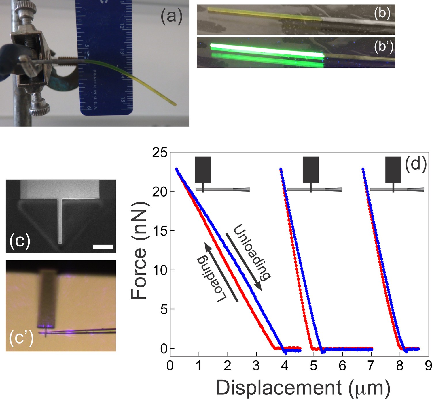
(a) A rod of fluorescent boron-dipyrromethene (BODIPY)-infused polydimethylsiloxane (PDMS) is suspended under its own weight. The Young’s modulus is readily extracted from the shape of the deformed beam, its dimensions, and the density of PDMS (see Materials and methods). (b–b') The rod from (a) was placed on a gel imager to illustrate its intense fluorescence under UV. (c–d) Atomic force microscopy (AFM) measurements on microfabricated cantilevers. (c) A custom AFM probe made from a commercially available AFM cantilever using ion beam milling. The narrow 2-mm-wide tip at the end of the probe provides a defined point of force application, at the same time ensuring firm grip between the AFM probe and the sample. Scale bar = 10 μm. (c’) AFM tip in contact with a microfabricated cantilever as seen through the optics of the AFM. Violet glare is the laser from the position sensitive detector of the AFM. (d) Three representative AFM measurements from a single cantilever. Schematics at the top illustrate the location where the microfabricated cantilever contacted the custom AFM tip. The three measurements are the corresponding force-displacement curves with the loading part shown in red, and the unloading portion shown in blue. The curves are shifted along the x-axis for better visibility (since the reference point on the x-axis is inessential). The two rightmost curves are repetitions with the AFM tip contacting the cantilever at the same location. The Young’s modulus for each cantilever examined (n=6) was calculated as described in the Materials and methods from the following information: the width of the cantilever; the distance from the AFM contact point to the junction with the glass scaffold, and the slope from the force-displacement curve.
Figure 4 with 2 supplements
Three-dimensional computational model of the Drosophila embryo.
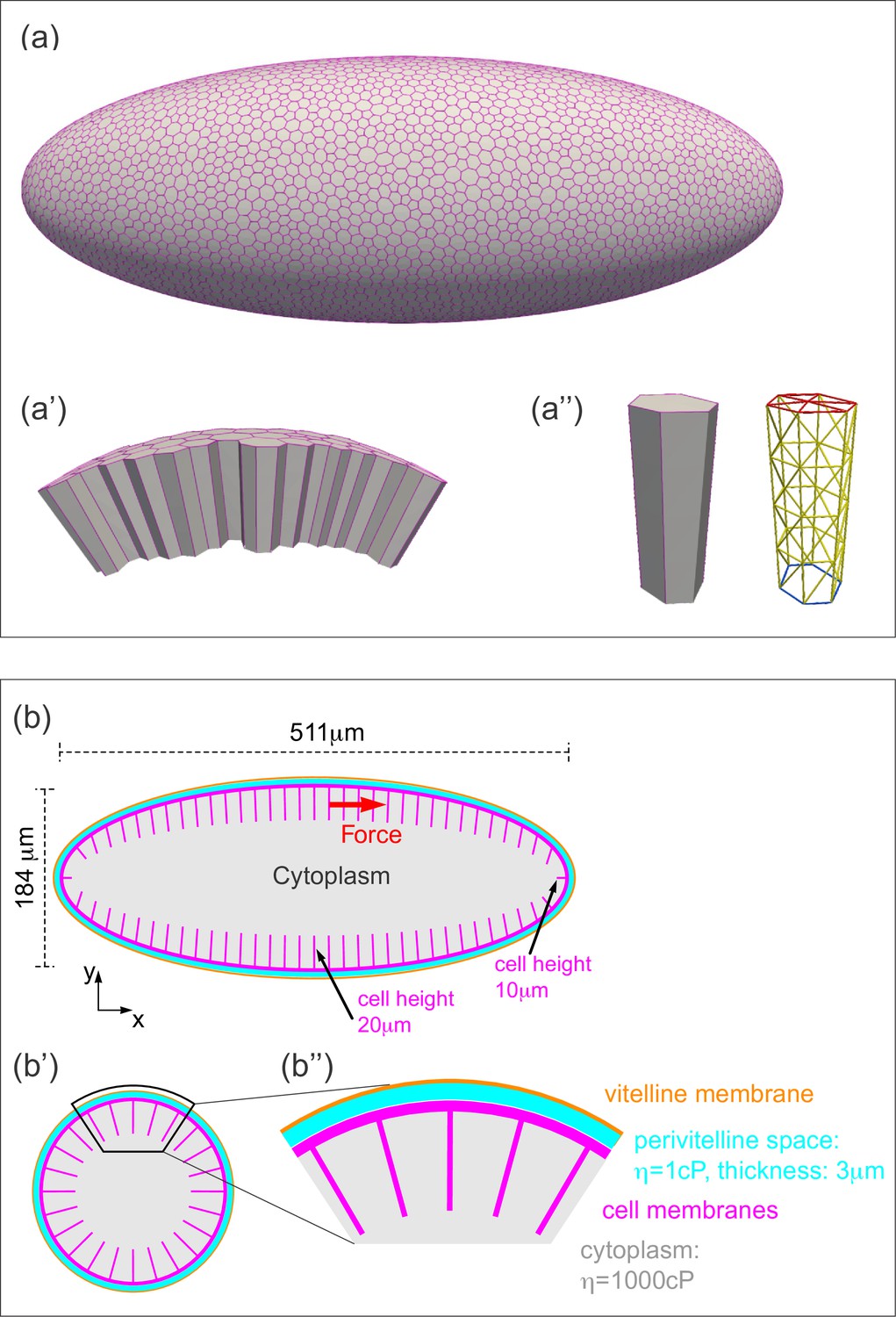
(a–a'') Illustrations of the cellular structures represented in the computational model. (a) An ellipsoid was tiled with a disordered hexagonal network to represent the cell boundaries on the surface of the embryo. (a') The cells themselves are three-dimensional prisms; a small portion of the surface, comprised of several cells, is shown here. (a'') Cells are represented as open prisms with lateral (yellow) and apical (red) surfaces modeled as networks of elastic springs, each with spring constant k; the basal (blue) surface of each cell is left open. (b–b'') Geometry of components of the simulated model embryo, not drawn to scale. (b) The long and short axis of the model embryo are 511 μm and 184 μm, respectively. Cell height is assigned in a gradient, with 20 μm heights in the middle diminishing to 10 μm heights at the poles. (b') Cartoon cross-section of model embryo and (b'') a portion of the cross-section. The vitelline membrane is 3 μm thick and filled with a fluid of 1 cP viscosity. The fluid in the interior of the embryo is assigned a viscosity of 1000 cP, agreeing with published measurements (Doubrovinski et al., 2017; Selvaggi et al., 2018). Details of numerical implementation and validation of the numerical method are described in the Materials and methods, Figure 4—figure supplement 1, and Figure 4—figure supplement 2.
Figure 4—figure supplement 1
Schematic explaining terms used in the numerical model.
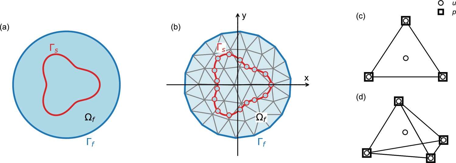
Our numerical approach combines the immersed boundary method and the finite element method, as described in the ‘Numerical model’ section of the Materials and methods. (a) Outer boundary of the computational domain (dark blue line) encloses fluid domain (light blue area); in our model, the computational domain is equivalent to the entire embryo. Boundary of the solid is denoted by (red line); in our model, the solid boundaries correspond to the cellular surfaces. (b) Same as (a), illustrating discretization of the solid and the fluid domains. (c,d) Two- and three-dimensional finite elements used in the simulations. Velocity (u) is defined on the nodes and on the center of mass, pressure (p) is defined only at the nodes.
Figure 4—figure supplement 2
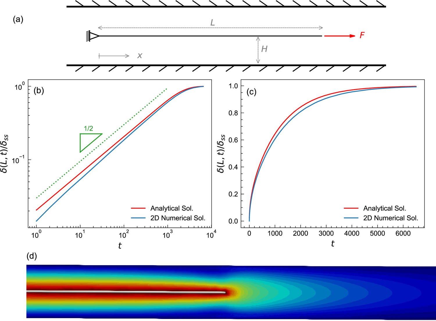
Test case to benchmark numerical method.
(a) A schematic of the fluid-structure interaction test problem showing a plate submerged in a fluid. The left end is fixed, the right end is subjected to a constant pulling force. The initial length of the plate is 5. The plate was placed in the center of a fluid domain having a length L of 8 and a height H of 0.05; the diagram shown is not to scale. The plate was discretized into a triangular mesh of linear springs whose spring constant was k=0.13, fluid viscosity was set to μ=1. The top and bottom boundaries of the fluid domain are Dirichlet (no-slip), while the left and the right boundaries are Neumann zero gradient boundaries (i.e., open boundaries). The fluid domain was discretized using a structured finite element mesh of right triangles with sides ∆x×∆y=0.005 × 0.0025. A constant pulling force of F=0.05 was applied to the right end of the plate. (b,c) Time evolution of a plate from (a) shown on logarithmic (b) and linear (c) scales, plotting normalized displacement of the rightmost point from initial position (with maximal displacement set to 1). The numerical solution (blue) agrees well with the analytical solution (red), which is described in the Appendix. (d) Iso-surfaces depicting the velocity magnitude profile around the plate, obtained from the numerical solution.
Figure 5
Results from parameter sweep with uniform elasticity explain relaxation dynamics or loading force but not both.
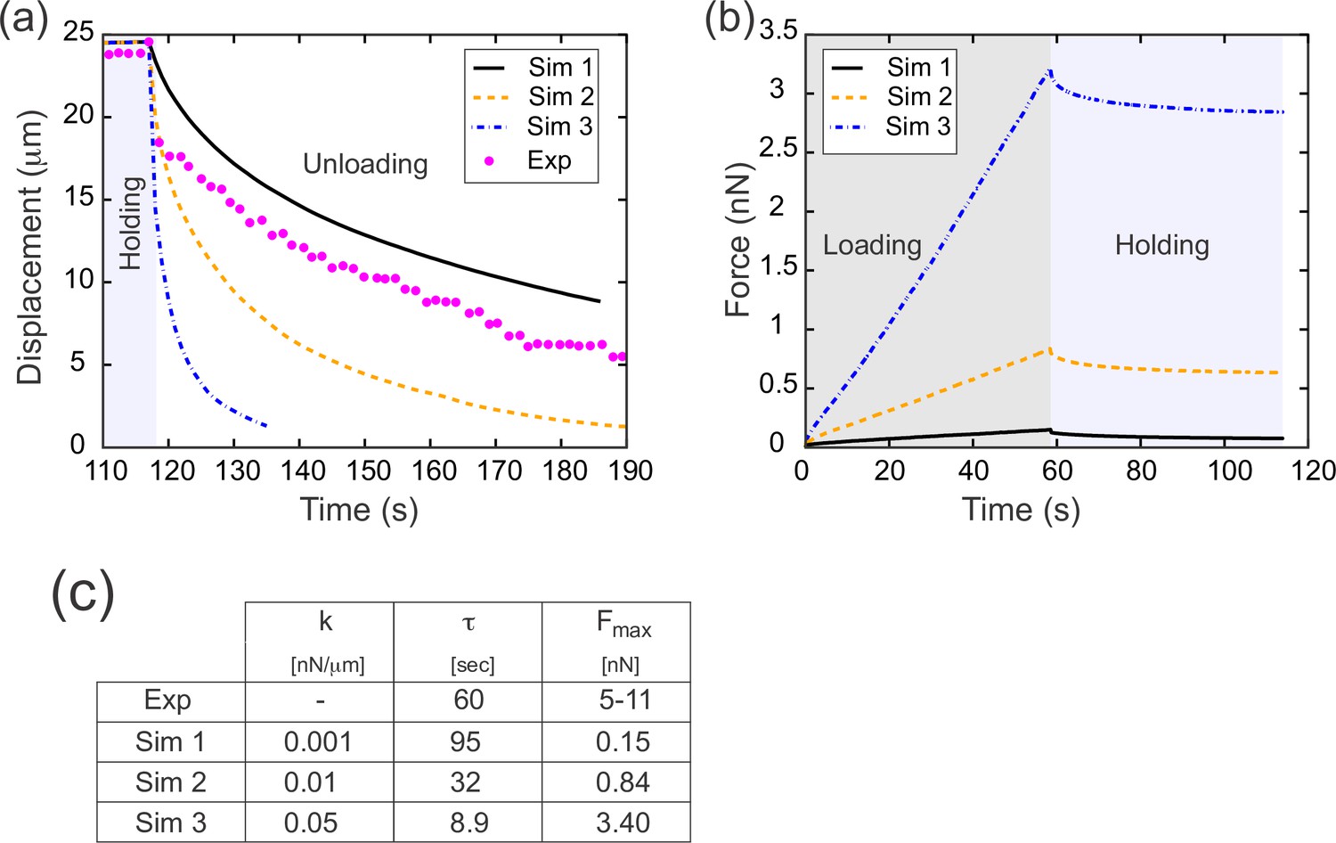
(a) Parameter fitting for the spring constant k. The computational model was run with a range of values for the single free parameter k; see text. The externally applied force was removed to assess relaxation of the pulled edge during unloading. A constant value equal to the asympototic value was subtracted from each curve; when plotted on a log plot, the slope of resulting line gives the exponential decay rate, τ. (b) Force versus time for the model in (a) during the loading (gray background) and holding (light blue background) phases. Compare with Figure 3c, which shows the equivalent experimentally measured forces. (c) Table of decay rates and maximal force for experiment and model parameter sweep. The value of k which best fits decay dynamics (0.001 nN/μm) drastically underestimates the loading force required.
Figure 6
Floppy and stiff networks contribute differently to loading and unloading dynamics.
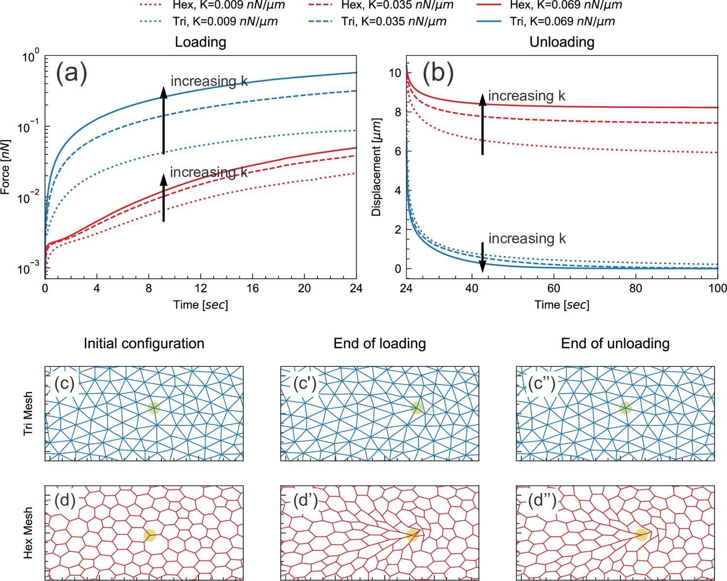
(a) Time evolution of force during the loading phase in simplified model tissues with triangular or hexagonal networks of springs. For both triangular (blue) and hexagonal (red) networks, the force required to impose a fixed displacement increases with increasing spring constant k. (b) Time evolution of force during the unloading phase in the same model tissues. Tissue relaxation is faster with increasing k in the triangular (blue) case, but slower with increasing k in the hexagonal (red) case. (c–d) Time points from the same model, showing the part of the network surrounding the node where force is applied (indicated by pale green circle). Images shown are from simulations where k=0.035 nN/μm. The triangular network largely returns to its original configuration by the end of unloading (c''), but the hexagonal network remains significantly deformed at the same time point (d'').
Figure 7 with 1 supplement
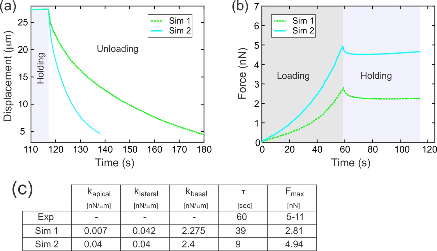
A difference in apical and basal elasticity determines tissue dynamics.
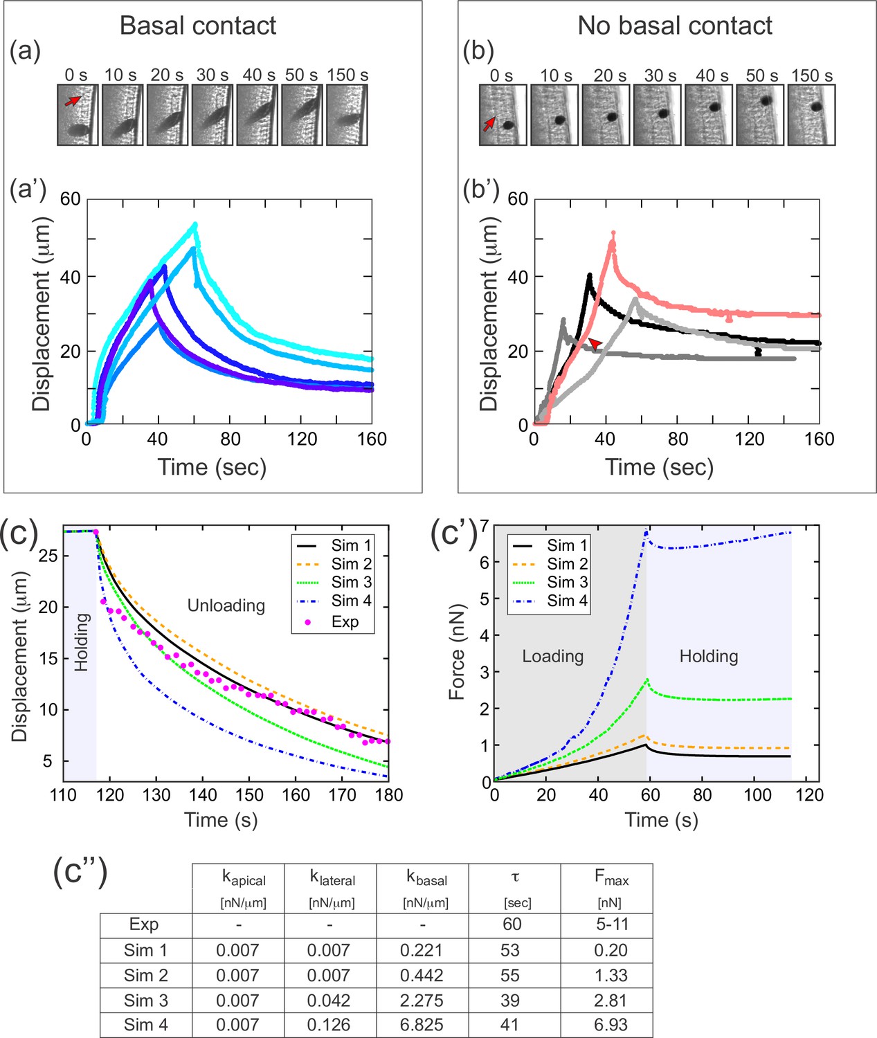
(a–a') Ferrofluid pulling experiment with droplets that contact the basal edge. The data in this panel has been previously reported (Doubrovinski et al., 2017). (a) Time frames from a typical experiment. The droplet was pulled toward the magnet and then released after approximately 50 s. The red arrow indicates the position of the cellularization front (i.e., the basal side of the newly forming cells). The droplet is clearly in contact with the basal side at all time points. (a') Displacement of the ferrofluid droplet is plotted as a function of time for several experiments. For easiest comparison, the experiments chosen for this plot most closely match the total displacements in b'. The speed of these droplets decreased as they approached the magnet, indicating a build-up of elastic stress in the epithelium. (b–b') Ferrofluid pulling experiment with smaller droplets that do not contact the basal edge. (b) Time frames from a typical experiment. The red arrow indicates the basal surface. In this sample, the droplet remains in the apical-lateral domain and does not contact the basal side at any time. (b') Ferrofluid droplet displacement measured in four different pulling experiments. In the gray/black curves, the droplet is never in contact with the basal side. These droplets do not slow down as they approach the magnet, indicating that elastic stress is not building up. The pink curve corresponds to a droplet that made mechanical contact with the basal side at the beginning of the experiment, but moved apically and lost contact with the basal surface at the time point indicated by the arrowhead. The acceleration that occurs at this time point is further evidence that the basal domain is more strongly elastic than the apical-lateral domain. (c–c'') Parameter fitting to assess mechanical contributions of lateral and basal structures. The computational model was run with a range of values for the parameters klateral and kbasal while holding kapical fixed. Compare with Figure 5 for fitting with a single spring constant k. Also see Figure 7—figure supplement 1 for an additional simulation varying kapical. (c) The externally applied force was removed to assess relaxation of the pulled edge during unloading. This data was used to calculate τ. (c') Force versus time for the model in (c) during the loading (gray background) and holding (light blue background) phases. (c'') Table of decay rates and maximal force for experiment and model parameter sweep. Increased elasticity within lateral and basal structures affects mechanics during loading (characterized by Fmax), with only minor effects on unloading (characterized by τ). Simulation 4 (blue curve) is our ‘best fit’, approximately matching both the rate of unloading and the maximal force seen in experiments.
Figure 7—figure supplement 1
The effects of apical elasticity on recoil.
The data here was generated in the same way as in Figure 7c–c’’. Simulation 1 in this figure supplement is the same as Simulation 3 in the main Figure 7c–c’’. Increasing kapical about sixfold (while holding kbasal and klateral approximately constant), resulted in a substantial (approximately fourfold) decrease in decay constant τ.
Figure 8
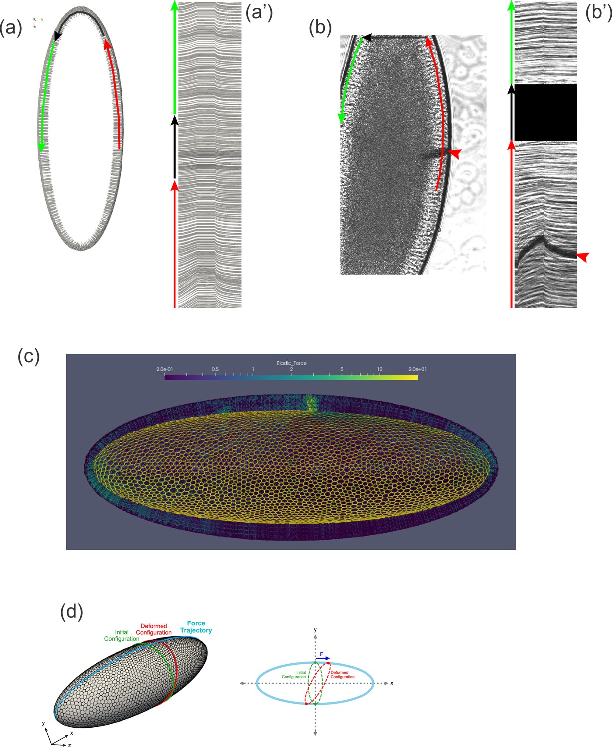
Tissue geometry constrains mechanical responses.
(a) A thin section through the sagittal plane of the model from Figure 7c (Simulation 4), shown at a single time point. The red, black, and green arrows indicate the curves used to generate the kymograph in (a'). (a') Kymograph corresponding to model data in (a). Traces at the top of the kymograph are not strictly horizontal, showing that motion is detected even on the opposite side of the model embryo from the force application. (b) A time point from a ferrofluid droplet pulling experiment. Ferrofluid droplet indicated by red arrowhead. The red, black, and green arrows indicate the curves used to generate the kymograph in (b'). (b') Kymograph corresponding to experimental data in (b). Traces at the top of the kymograph are not strictly horizontal, showing that motion is detected even on the opposite side of the embryo from the droplet-applied force. (c) Color plot indicating the distribution of stress across the model embryo from Figure 7c (Simulation 4), averaged over the last 5 s of the pulling phase. Note that stress spreads across the whole tissue and is upregulated at the poles. (d) A schematic explaining how tissue geometry can affect the dynamics. An imaginary ellipsoid encircling the embryo is shown at two points: at the initial time point (green) and during force loading (red). Applying force at one point causes the imaginary ellipse to stretch, leading to an increase in elastic stress.
Videos
Video 1
Cantilever pulling experiment.
Cell outlines are marked magenta (CellMask dye). Cantilever is green (boron-dipyrromethene [BODIPY] dye).
Video 2
Cantilever pulling experiment with nuclei.
Cell outlines are marked magenta (CellMask dye). Cantilever is green (boron-dipyrromethene [BODIPY] dye). Nuclei (Histone-RFP) are cyan. Nuclei deform as the tissue is pulled and they restore their shape after the tissue is allowed to relax.
Video 3
Simulation of pulling experiment.
The color indicates elastic stress distribution, calculated as E*(L-L0) for each elastic spring, where E is the spring constant, L0 is the rest length, and L is instantaneous length. Note that stress is elevated (green) near the poles in the lateral membranes particularly during the holding phase.
Video 4
Ferrofluid pulling experiment.
Brightfield is shown in grayscale, CellMask dye fluorescence is shown in red. Note that the tissue is moving even on the opposite side of the embryo as the tissue is being pulled locally.
Tables
Key resources table
| Reagent type (species) or resource | Designation | Source or reference | Identifiers | Additional information |
|---|---|---|---|---|
| Genetic reagent (Drosophila melanogaster) | gap43-Cherry | Gift from the lab of Eric F. Wieschaus | https://www.nature.com/articles/nature07522 | |
| Chemical compound, drug | Cell Mask Plasma Membrane Stain (Deep Red) | Thermo Fisher Scientific | C10046 | https://www.thermofisher.com/order/catalog/product/C10046 |
Additional files
Download links
A two-part list of links to download the article, or parts of the article, in various formats.
Downloads (link to download the article as PDF)
Open citations (links to open the citations from this article in various online reference manager services)
Cite this article (links to download the citations from this article in formats compatible with various reference manager tools)
A comprehensive model of Drosophila epithelium reveals the role of embryo geometry and cell topology in mechanical responses
eLife 12:e85569.
https://doi.org/10.7554/eLife.85569


