Core PCP mutations affect short-time mechanical properties but not tissue morphogenesis in the Drosophila pupal wing
Figures
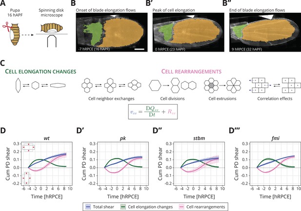
Core planar cell polarity (PCP) does not orient cellular behaviors and tissue reshaping during pupal blade elongation flows: (A) Cartoon of pupal wing dissection at 16 hAPF and imaging using a spinning disk microscope.
(B–B″) Images of a wt wing at −7, 0, and 9 hRPCE (for this movie these times correspond to 16, 23, and 32 hAPF). The green and orange regions correspond to the hinge and blade, respectively. Anterior is up; proximal to the left. Scale bar, 100 μm. (C) Schematic of the cellular contributions underlying anisotropic tissue deformation. The tissue shear rate component , which quantifies the rate of anisotropic tissue deformation along the proximal–distal wing axis, is decomposed into deformations arising from the rate of change of cell shapes and the deformations arising from the cellular rearrangements (Etournay et al., 2015; Merkel et al., 2017). Total shear is the sum of cell elongation changes (green) and cell rearrangements (magenta). (D–D′″) Accumulated proximal–distal (Cum PD) tissue shear during blade elongation flows in the blade region averaged for (D) wt (n = 4), (D′) pk (n = 3), (D″) stbm (n = 3), and (D′″) fmi (n = 2) movies. Solid line indicates the mean, and the shaded regions enclose ± standard error of the mean (SEM). Differences in total accumulated shear are not statistically significant (Figure 1—figure supplement 2C). Time is relative to peak cell elongation (hRPCE).
-
Figure 1—source data 1
Numerical data for Figure 1D–D′′′, accumulated proximal–distal tissue shear during blade elongation flows in the blade region for wt and core PCP mutants.
- https://cdn.elifesciences.org/articles/85581/elife-85581-fig1-data1-v3.zip
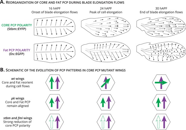
Reorganization of the core and Fat planar cell polarity (PCP) systems during pupal blade elongation flows.
(A) Evolution of the PCP network during pupal blade elongation flows (Merkel et al., 2014; Aigouy et al., 2010). Core PCP polarity is based on Stbm::YFP. Initially, core PCP polarity is organized toward the wing margin. As tissue flows occur, it reorients toward the distal tip. Fat PCP polarity is based on the pattern of Ds::EGFP. Fat PCP is initially also margin organized. By the end of the blade elongation, Fat PCP is perpendicularly oriented to core PCP. Cartoon adapted from Merkel et al., 2014. (B) Schematic of the core (green arrow) and Fat (purple arrow) PCP patterns in wt, pk, stbm, and fmi wings (Merkel et al., 2014). During pupal tissue flows in wt wings, core PCP reorients toward the distal tip of the wing. By the end of blade elongation flows, core and Fat PCP are perpendicularly aligned. In pk mutant wings, core and Fat PCP remain aligned and core polarity is reduced. In stbm and fmi wings, the core PCP network is strongly reduced (empty green arrow), whereas the Fat PCP pattern is unperturbed (purple arrow).
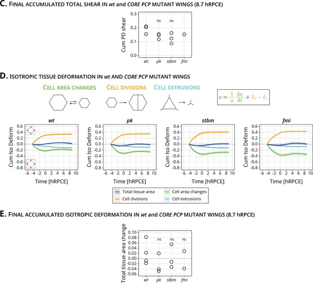
Quantification of final pupal tissue deformation and cellular contributions to isotropic tissue area.
(C) Statistical analysis of the final accumulated proximal–distal (Cum PD) tissue shear in wt (n = 4 ), pk (n = 3), stbm (n = 3), and fmi (n = 2) movies. Significance is estimated using the Kruskal–Wallis test. ns, p-val >0.05. (D) Isotropic tissue deformation is decomposed into contributions from change in cell area , cell division rate , and cell extrusion rate . Quantification of accumulated isotropic tissue deformation and its components in wt (n = 4), pk (n = 3), stbm (n = 3), and fmi (n = 2) movies. The cellular contributions are cell area changes (green), cell divisions (yellow), and cell extrusions (cyan). Solid line indicates the mean, and the shaded regions enclose ± standard error of the mean (SEM). The time is relative to peak cell elongation (hRPCE). (E) Statistical analysis of the final pupal accumulated tissue area change in wt (n = 4), pk (n = 3), stbm (n = 3), and fmi (n = 2) movies. Significance is estimated using an analysis of variance (ANOVA) test. ns, p-val >0.05.
-
Figure 1—figure supplement 2—source data 1
Numerical data of Figure 1—figure supplement 2C.
- https://cdn.elifesciences.org/articles/85581/elife-85581-fig1-figsupp2-data1-v3.zip
-
Figure 1—figure supplement 2—source data 2
Numerical data of Figure 1—figure supplement 2D.
- https://cdn.elifesciences.org/articles/85581/elife-85581-fig1-figsupp2-data2-v3.zip
-
Figure 1—figure supplement 2—source data 3
Numerical data of Figure 1—figure supplement 2E.
- https://cdn.elifesciences.org/articles/85581/elife-85581-fig1-figsupp2-data3-v3.zip
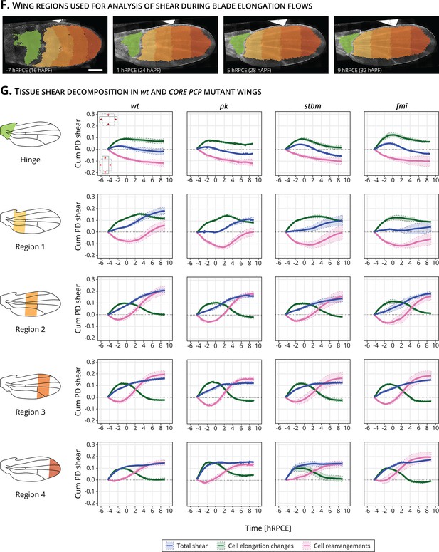
Regional analysis of tissue shear in the hinge and four blade subregions.
(F) Images of a wt wing at −7, 1, 5, and 9 hRPCE (relative to peak cell elongation), corresponding to 16, 24, 28, and 32 hAPF in this movie. The green region corresponds to the hinge, and the four blade subregions are shown in an orange color palette. Scale bar, 100 μm. (G) Total accumulated proximal–distal (Cum PD) tissue shear (dark blue curve) and its decomposition into cell elongation changes (green curve) and cell rearrangements (magenta curve) for the hinge and four blade subregions for wt (n = 4), pk (n = 3), stbm (n = 3), and fmi (n = 2). Solid line indicates the mean, and the shaded regions enclose ± standard error of the mean (SEM). Time is relative to peak cell elongation (hRPCE).
-
Figure 1—figure supplement 3—source data 1
Numerical data of Figure 1—figure supplement 3G.
- https://cdn.elifesciences.org/articles/85581/elife-85581-fig1-figsupp3-data1-v3.zip
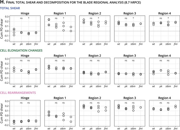
Statistics of final shear in the blade subregions and its cellular contributions.
(H) Quantification of the final accumulated proximal–distal (Cum PD) total shear (top row), shear caused by cell elongation changes (middle row), and shear caused by cell rearrangements (bottom row) in the hinge (left column) and four blade subregions for wt (n = 4), pk (n = 3), stbm (n = 3), and fmi (n = 2). Significance is estimated using the Kruskal–Wallis test. *p-val ≤0.05; ns, p-val >0.05.
-
Figure 1—figure supplement 4—source data 1
Numerical data of Figure 1—figure supplement 4H.
- https://cdn.elifesciences.org/articles/85581/elife-85581-fig1-figsupp4-data1-v3.zip
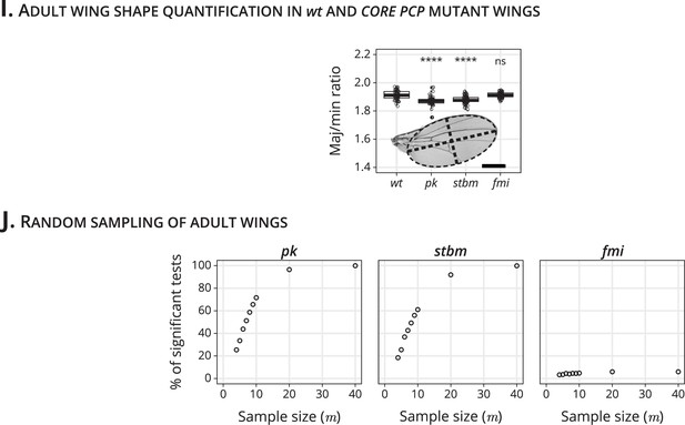
Adult wing shape quantification and random sampling.
(I) Quantification of the adult wing blade major (maj) to minor (min) ratio for wt, pk, stbm, and fmi wings (n ≥ 47). Scale bar, 500 μm. Each empty circle indicates one wing, and the box plots summarize the data: thick black line indicates the median; the boxes enclose the first and third quartiles; lines extend to the minimum and maximum without outliers, and filled circles mark outliers. Significance is estimated using the Kruskal–Wallis test. ****p-val ≤0.0001; ns, p-val>0.05. (J) Percentage of statistically significant tests obtained by comparing random sampling of wt and the three PCP mutant adult wings. The statistical analysis was run 10,000 times with all the sample sizes studied (3, 4, 5, 6, 7, 8, 9, 10, 20, and 40). The random sample size was the same for all genotypes. The statistical significance was computed using the wt genotype as a reference group.
-
Figure 1—figure supplement 5—source data 1
Numerical data of Figure 1—figure supplement 5I.
- https://cdn.elifesciences.org/articles/85581/elife-85581-fig1-figsupp5-data1-v3.zip
-
Figure 1—figure supplement 5—source data 2
Numerical data of Figure 1—figure supplement 5J.
- https://cdn.elifesciences.org/articles/85581/elife-85581-fig1-figsupp5-data2-v3.zip
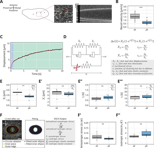
Rheological model for the response to laser ablation: (A) Schematic of a wt wing at −8 hRPCE.
Linear laser ablation experiments were performed in the blade region enclosed by the red square. Dots on the wing cartoon indicate sensory organs. The red line corresponds to the ablation, and the kymograph was drawn perpendicularly to the cut (yellow). Scale bar, 5 μm. (B) Initial recoil velocity upon ablation (simplified as recoil velocity in the y-axis title) along the proximal–distal (PD) axis at −8 hRPCE for wt (gray) and pk (blue) tissues (n ≥ 9). Significance is estimated using the Mann–Whitney U-test. ***p-val ≤0.001. (C) Example of the measured displacement after laser ablation (black dots) and corresponding exponential fit of the mechanical model (red curve). The blue and green regions highlight the displacement in the fast and slow timescale, respectively. (D) Description of the mechanical model that was devised to analyze the tissue response upon laser ablation. After the cut, the spring with elastic constant is ablated (red scissor), and the tissue response is given by the combination of the two Kelvin–Voigt models arranged in series. These two correspond to the fast response given by and and the slow response given by and . The mechanical stress is constant. The membrane displacement is calculated as a sum of the displacement () associated with the fast timescale () and the displacement () associated with the slow timescale (). (E–E′′′) Values obtained for each of the four fitting parameters when fit to the data. (E) Displacement associated with the fast and (E′) slow timescale for wt (gray) and pk (blue). (E′′) Fast and (E′′′) slow timescale for wt (gray) and pk (blue) (n ≥ 5). Significance is estimated using the Student’s t-test. **p-val ≤0.01; ns, p-val >0.05. (F) Example of a circular laser ablation used for analysis with elliptical shape after circular ablation (ESCA). The left image shows the final shape of the ablation around 2 min after cut, and the right image shows the corresponding segmented image, where the inner and outer pieces were fit with ellipses. After the fitting, the model outputs the anisotropic and isotropic stress (equations shown on the right side). Scale bar, 20 μm. A = anterior, P* = posterior, D = distal, P = proximal. (F′) Anisotropic stress for wt (gray) and pk (blue) tissues at −8 hRPCE (n ≥ 4). Significance is estimated using the Mann–Whitney U-test. ns, p-val >0.05. (F″) Isotropic stress for wt (gray) and pk (blue) tissues at −8 hRPCE (n ≥ 4). Significance is estimated using the Mann–Whitney U-test. ns, p-val >0.05. Time is relative to peak cell elongation (hRPCE). In all plots, each empty circle indicates one cut, and the box plots summarize the data: thick black line indicates the median; the boxes enclose the first and third quartiles; lines extend to the minimum and maximum without outliers, and filled circles mark outliers.
-
Figure 2—source data 1
Numerical data for Figure 2B, initial recoil velocity upon ablation along the proximal–distal (PD) axis for wt and pk tissues.
- https://cdn.elifesciences.org/articles/85581/elife-85581-fig2-data1-v3.zip
-
Figure 2—source data 2
Numerical data for Figure 2E, values for fitted parameters of the rheological model.
- https://cdn.elifesciences.org/articles/85581/elife-85581-fig2-data2-v3.zip
-
Figure 2—source data 3
Numerical data for Figure 2F–F″, values for anisotropic and isotropic stress deteremined with elliptical shape after circular ablation (ESCA).
- https://cdn.elifesciences.org/articles/85581/elife-85581-fig2-data3-v3.zip
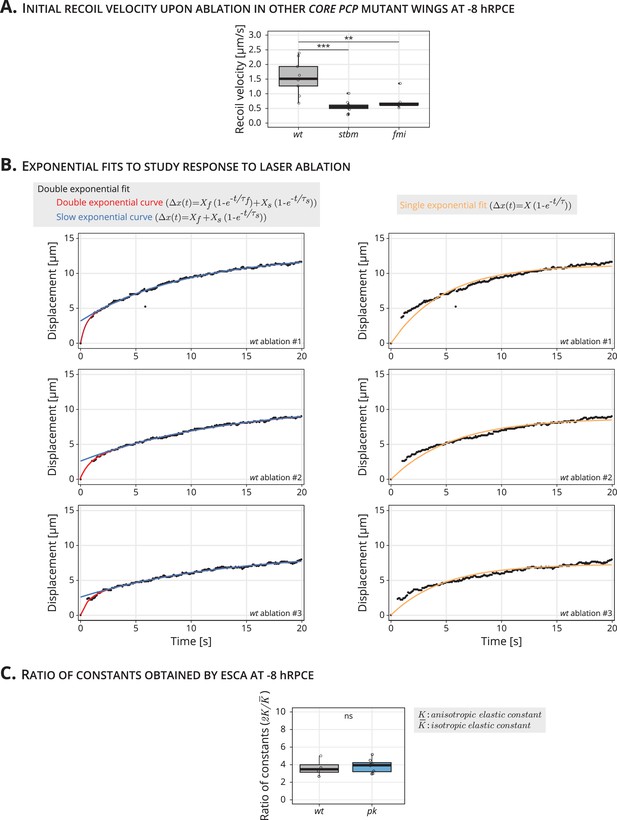
Initial recoil velocity upon linear laser ablation for stbm and fmi mutant wings, exponential fits of cell response upon laser ablation, and ratio of elastic constants obtained by elliptical shape after circular ablation (ESCA) at −8 hRPCE.
(A) Initial recoil velocity upon ablation (simplified as recoil velocity in the y-axis title) along the proximal–distal (PD) axis for wt (gray), stbm (green), and fmi (purple) mutant wings at −8 hRPCE (n ≥ 9). Significance is estimated using the Kruskal–Wallis test. ***p-val ≤0.001; **p-val ≤0.01. (B) Example of exponential fits of the cell response to laser ablation in three different wt wings at −8 hRPCE. The left plots shows the double exponential plot used with the Kelvin–Voigt model (red) and the slow exponential curve generated using the parameters from the double exponential fit (blue). The right plots show a single exponential fit (orange). These plots show that the double exponential fit captures both the fast and slow response to laser ablation. (C) Ratio of elastic constants () for wt and pk (blue) at −8 hRPCE (n ≥ 4). Significance is estimated using the Mann–Whitney U-test. ns, p-val >0.05. Time is relative to Peak Cell Elongation (hRPCE). In (A) and (C), each empty circle indicates one cut, and the box plots summarize the data: thick black line indicates the median; the boxes enclose the first and third quartiles; lines extend to the minimum and maximum without outliers, and filled circles mark outliers.
-
Figure 2—figure supplement 1—source data 1
Numerical data of Figure 2—figure supplement 1A.
- https://cdn.elifesciences.org/articles/85581/elife-85581-fig2-figsupp1-data1-v3.zip
-
Figure 2—figure supplement 1—source data 2
Numerical data of Figure 2—figure supplement 1B.
- https://cdn.elifesciences.org/articles/85581/elife-85581-fig2-figsupp1-data2-v3.zip
-
Figure 2—figure supplement 1—source data 3
Numerical data of Figure 2—figure supplement 1C.
- https://cdn.elifesciences.org/articles/85581/elife-85581-fig2-figsupp1-data3-v3.zip
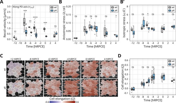
Dynamics of stress and cell elongation throughout blade elongation flows in wt and pk mutant.
(A) Initial recoil velocity upon ablation (simplified as recoil velocity in the y-axis title) along the proximal–distal (PD) axis throughout blade elongation flows for wt (gray) and pk (blue) tissues (n ≥ 3). Significance is estimated using the Mann–Whitney U-test. ****p-val ≤0.0001; ***p-val ≤0.001; **p-val ≤0.01; ns, p-val >0.05. (B) Elliptical shape after circular ablation (ESCA) results for anisotropic stress for wt (gray) and pk (blue) tissues throughout blade elongation flows (n ≥ 3). Significance is estimated using the Mann–Whitney U-test. *p-val <0.05; ns, p-val >0.05. (B′) ESCA results for isotropic stress for wt (gray) and pk (blue) throughout blade elongation flows (n ≥ 3). Significance is estimated using the Mann–Whitney U-test. *p-val <0.05; ns, p-val >0.05. (C) Color-coded PD component of cell elongation in the blade region between the second and third sensory organs found in the intervein region between L2 and L3. The images correspond to wt (top row) and pk (bottom row) wings throughout blade elongation flows. Scale bar, 5 μm. (D) Quantification of the PD component of cell elongation in this region throughout blade elongation flows for wt (gray) and pk (blue) (n ≥ 3). Significance is estimated using the Mann–Whitney U-test. ns, p-val >0.05. Time is relative to peak cell elongation (hRPCE). In all plots, each empty circle indicates one experiment, and the box plots summarize the data: thick black line indicates the median; the boxes enclose the first and third quartiles; lines extend to the minimum and maximum without outliers, and filled circles mark outliers.
-
Figure 3—source data 1
Numerical data for Figure 3A, initial recoil velocity upon ablation along the proximal–distal (PD) axis throughout blade elongation flows for wt and pk mutant tissues.
- https://cdn.elifesciences.org/articles/85581/elife-85581-fig3-data1-v3.zip
-
Figure 3—source data 2
Numerical data for Figure 3B–B′, elliptical shape after circular ablation (ESCA) results for anisotropic and isotropic stress in wt and pk mutant tissues throughout blade elongation flows.
- https://cdn.elifesciences.org/articles/85581/elife-85581-fig3-data2-v3.zip
-
Figure 3—source data 3
Numerical data for Figure 3D, proximal–distal (PD) component of cell elongation Q throughout blade elongation flows for wt and pk mutant tissues.
- https://cdn.elifesciences.org/articles/85581/elife-85581-fig3-data3-v3.zip
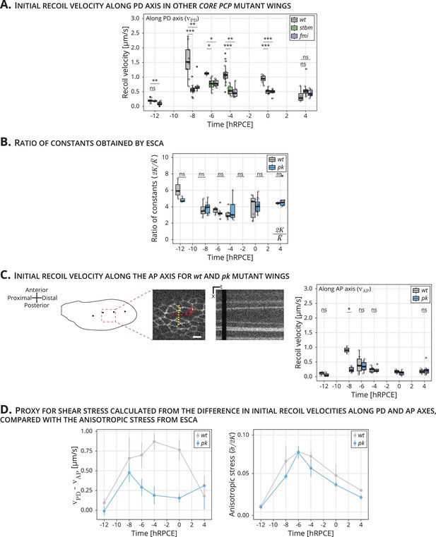
Study of pupal wing mechanics over time.
(A) Initial recoil velocity upon ablation (simplified as recoil velocity in the y-axis title) along the proximal–distal (PD) axis for wt (gray), stbm (green), and fmi (purple) mutant wings throughout blade elongation flows (n ≥ 4). Significance is estimated using the Kruskal–Wallis test. ***p-val ≤0.001; **p-val ≤0.01; *p-val ≤0.05; ns, p-val >0.05. (B) Ratio of elastic constants () for wt and pk (blue) throughout blade elongation flows (n≥3). Significance is estimated using the Kruskal–Wallis test. ns, p-val >0.05. Time is relative to peak cell elongation (hRPCE). (C) Left: Schematic of a wt wing at −8 hRPCE. Linear laser ablation experiments were performed in the blade region enclosed by the red square. Dots on the cartoon indicate sensory organs. Red line corresponds to the ablation; the kymograph was drawn perpendicularly to the cut (yellow). Scale bar, 5 μm. Right: Initial recoil velocity upon ablation (simplified as recoil velocity in the y-axis title) along the anterior–posterior (AP) axis for wt (gray) and pk (blue) mutant wings throughout blade elongation flows (n ≥ 3, n = 2 in wt wings at 0 hr). Significance is estimated using the Mann–Whitney U-test. *p-val ≤0.05; ns, p-val >0.05. (D) Proxy for shear stress calculated as the difference between the initial recoil velocity along the PD (vPD) and AP (vAP) axes for wt (gray) and pk (blue) mutant wings (left plot), compared to the anisotropic stress () outputted by elliptical shape after circular ablation (ESCA; right plot). Filled colored dots correspond to the mean value, and the error bars report the standard error of the mean (SEM). Significance is estimated using the Kruskal–Wallis test. **p-val ≤0.01; *p-val ≤0.05; ns, p-val >0.05. Time is relative to peak cell elongation (hRPCE). In (A–C), each empty circle indicates one experiment, and the box plots summarize the data: thick black line indicates the median; the boxes enclose the first and third quartiles; lines extend to the minimum and maximum without outliers, and filled circles mark outliers.
-
Figure 3—figure supplement 1—source data 1
Numerical data of Figure 3—figure supplement 1A, initial recoil velocity upon ablation along the proximal–distal (PD) axis throughout blade elongation flows for wt, stbm, and fmi tissues.
- https://cdn.elifesciences.org/articles/85581/elife-85581-fig3-figsupp1-data1-v3.zip
-
Figure 3—figure supplement 1—source data 2
Numerical data of Figure 3—figure supplement 1B, elliptical shape after circular ablation (ESCA) report of ratio of elastic constants throughout blade elongation flows for wt and pk.
- https://cdn.elifesciences.org/articles/85581/elife-85581-fig3-figsupp1-data2-v3.zip
-
Figure 3—figure supplement 1—source data 3
Numerical data of Figure 3—figure supplement 1C, initial recoil velocity along the anterior–posterior (AP) axis for wt and pk.
- https://cdn.elifesciences.org/articles/85581/elife-85581-fig3-figsupp1-data3-v3.zip
-
Figure 3—figure supplement 1—source data 4
Numerical data of Figure 3—figure supplement 1D, proxy for shear stress calculated as the difference between the initial recoil velocities along the proximal–distal (PD) and anterior–posterior (AP) axes for wt and pk, and elliptical shape after circular ablation (ESCA) report of anisotropic stress throughout blade elongation flows for wt and pk.
- https://cdn.elifesciences.org/articles/85581/elife-85581-fig3-figsupp1-data4-v3.zip
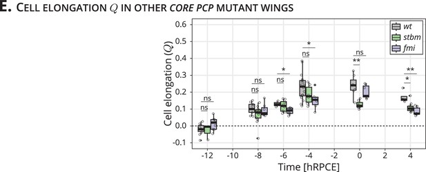
Quantification of cell elongation in the blade region throughout blade elongation flows.
(E) Quantification of in the blade throughout blade elongation flows for wt (gray), stbm (green), and fmi (purple) mutant wings (n ≥ 4). Significance is estimated using the Kruskal–Wallis test. **p-val ≤0.01; *p-val ≤0.05; ns, p-val >0.05. Time is relative to peak cell elongation (hRPCE). Each empty circle indicates one experiment, and the box plots summarize the data: thick black line indicates the median; the boxes enclose the first and third quartiles; lines extend to the minimum and maximum without outliers, and filled circles mark outliers.
-
Figure 3—figure supplement 2—source data 1
Numerical data of Figure 3—figure supplement 2E, proximal–distal (PD) component of cell elongation Q throughout blade elongation flows for wt, stbm, and fmi tissues.
- https://cdn.elifesciences.org/articles/85581/elife-85581-fig3-figsupp2-data1-v3.zip
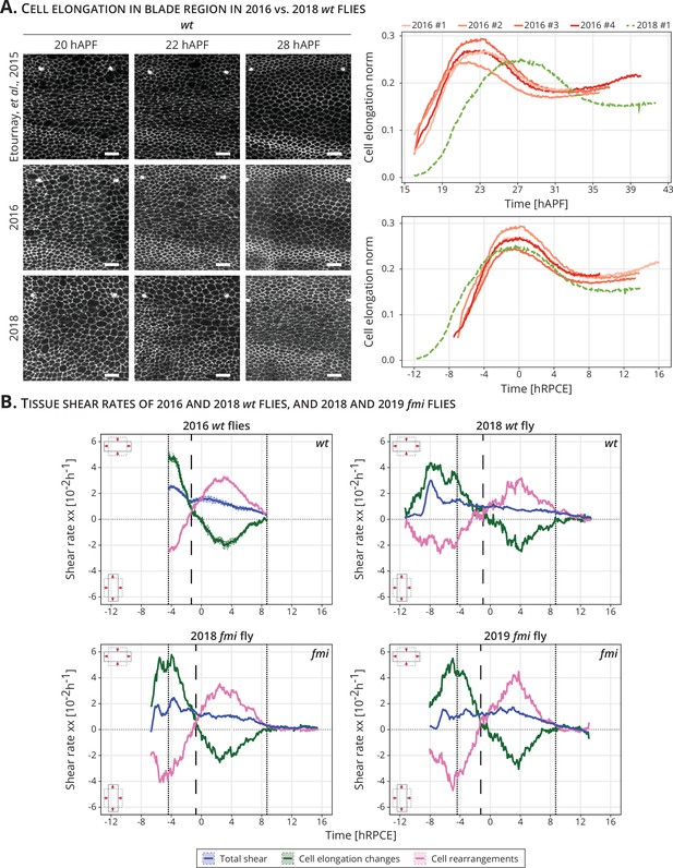
Delay and time alignment of old and newer flies: (A) Left: Snapshots of the blade region of long-term timelapses of wt pupal wing morphogenesis acquired in different years.
Scale bar, 10 μm. Right: Cell elongation norm during blade elongation flows for old flies (orange palette, 2016 flies) and new flies (green curve, 2018 fly). Top plot: Cell elongation magnitude for each movie not aligned in time. The peak of cell elongation is delayed from around 23 to 28 hAPF. Bottom plot: Cell elongation magnitude after alignment in time to the peak of cell elongation. Time is now expressed in hours relative to peak cell elongation (hRPCE). (B) Cell dynamics underlying anisotropic tissue deformation for 2016 wt (n = 4, top left), 2018 wt flies (n = 1, top right), and 2 fmi flies imaged in 2018 (bottom left) and 2019 (bottom right). The vertical dashed line marks the timepoint where cell rearrangements flip from AP- to PD-oriented per movie. The two dotted lines mark the start and the end of the analyzed wt long-term timelapses acquired in 2016. The time is relative to the peak of cell elongation (hRPCE).
Videos
Shown here is an example of a linear laser ablation, cutting three to four cells, in wt (left) or pk pupal wings.
The movie goes dark during the ablation itself. Thereafter, the tissue displaces. Anterior is up; proximal is left.
Tables
| Reagent type (species) or resource | Designation | Source or reference | Identifiers | Additional information |
|---|---|---|---|---|
| gene (Drosophila melanogaster) | w- | NA | FLYB:FBal0018186 | |
| gene (Drosophila melanogaster) | shg (shotgun; E-cadherin) | NA | FLYB:FBgn0003391 | |
| gene (Drosophila melanogaster) | pk30 | NA | FLYB:FBal0101223 | |
| gene (Drosophila melanogaster) | stbm6 | NA | FLYB:FBal0062423 | |
| gene (Drosophila melanogaster) | fmifrz3 | NA | FLYB:FBal0143193 | |
| strain, strain background (Drosophila melanogaster, male) | wt | Other | PMID:19429710 | Huang et al., 2009. Genotype: wt: w-; EcadGFP; |
| strain, strain background (Drosophila melanogaster, male) | pk | Bloomington Drosophila Stock Center | RRID:BDSC_44229 | Gubb et al., 1999. Genotype: w-; EcadGFP, pk30; |
| strain, strain background (Drosophila melanogaster, male) | stbm | Bloomington Drosophila Stock Center | RRID:BDSC_6918 | Wolff and Rubin, 1998. Genotype: w-; EcadGFP, stbm6; |
| strain, strain background (Drosophila melanogaster, male) | fmi | Bloomington Drosophila Stock Center | RRID:BDSC_6967 | Wolff and Rubin, 1998. Genotype: w-; EcadGFP, fmifrz3; |
| chemical compound, drug | Euparal | Carl Roth | 7356.1 | |
| chemical compound, drug | Holocarbon oil 700 | Sigma-Aldrich | H8898 | |
| chemical compound, drug | Isopropanol (2-propanol) | Sigma-Aldrich | 1.0104 | |
| software, algorithm | Fiji | Other | v. 2.0.0-rc-68/1.52e | Schindelin et al., 2012 |
| software, algorithm | Ilastik | Other | v. 1.2.2 | Berg et al., 2019 |
| software, algorithm | MATLAB | Other | v. 9.2.0.1226206 (R2017a) | MATLAB, 2017 |
| software, algorithm | PreMosa | Other | Blasse et al., 2017 | |
| software, algorithm | R | Other | v. 3.4.1 | R Development Core Team, 2020 |
| software, algorithm | Rstudio | Other | v. 3.6.1 | RStudio Team, 2020 |
| software, algorithm | TissueMiner | Other | v. TM_1.0.2 | Etournay et al., 2016 |
| other | Coverslip | Paul Marienfeld GmbH | 107052 | |
| other | Microscope slides | Paul Marienfeld GmbH | 1000200 | |
| other | Dumont #55 Forceps | Fine Science Tools | 11295–51 | |
| other | Vannas Spring Scissors | Fine Science Tools | 15000–08 |
Date of acquisition of all long-term timelapses.
| Genotype | Date of acquisition | Start [hAPF] | End [hAPF] |
|---|---|---|---|
| wt | March 30, 2016 | 16 | 39.83 |
| April 2, 2016 | 16 | 36.58 | |
| April 3, 2016 | 16 | 36.50 | |
| April 13, 2016 | 16 | 32.58 | |
| June 20, 2018 | 16 | 41.17 | |
| pk | April 9, 2016 | 16 | 39.00 |
| June 28, 2016 | 16 | 36.00 | |
| June 29, 2016 | 16 | 39.92 | |
| stbm | November 25, 2015 | 16 | 40.67 |
| November 28, 2015 | 16 | 35.33 | |
| December 11, 2014 | 16 | 37.58 | |
| fmi | October 20, 2018 | 16 | 39.17 |
| July 20, 2019 | 16 | 38.17 |
Parameters used to perform laser ablations.
| Linear ablations | Circular ablations | |
|---|---|---|
| Exposure time [s] | 0.05 | 0.05 |
| 488-nm laser intensity [%] | 50 | 50 |
| Time interval [s] | 0.09 | 2.55 |
| Pulses per shot | 25 | 25 |
| Shots per µm | 2 | 2 |
| Shooting time [s] | 0.67 | 147.28 |
| Thickness of stack ablated [µm] | 1 | 20 |
Additional files
-
MDAR checklist
- https://cdn.elifesciences.org/articles/85581/elife-85581-mdarchecklist1-v3.pdf
-
Source code 1
Fiji macro used to quantify size and shape of adult wings.
Inputs raw image of an adult wing and outputs text document containing quantifications of area, perimeter, major axis length, minor axis length, and other measurements not used in this manuscript.
- https://cdn.elifesciences.org/articles/85581/elife-85581-code1-v3.zip
-
Source code 2
Fiji macro used to draw kymographs from a laser ablation experiment.
Inputs stack of images from a timelapse laser ablation experiment. Outputs kymograph image that is later used to compute the initial recoil velocity upon ablation (Source code 3).
- https://cdn.elifesciences.org/articles/85581/elife-85581-code2-v3.zip
-
Source code 3
Matlab script used to calculate the initial recoil velocity upon laser ablation in linear cuts.
Inputs include the path to a folder containing the kymograph for each cut, as well as the pixel size in microns and time interval between image acquisition. Outputs a mat file containing the initial recoil velocity calculated as the average between the recoil velocities of the two membranes of the ablated cell.
- https://cdn.elifesciences.org/articles/85581/elife-85581-code3-v3.zip
-
Source code 4
Matlab script used to concatenate all calculated initial recoil velocities for a given dataset.
Inputs the path to a folder containing the mat files output from first script (Source code 3). Outputs a list of recoil velocities for each analyzed laser ablation experiment.
- https://cdn.elifesciences.org/articles/85581/elife-85581-code4-v3.zip


