Dynamic organization of cerebellar climbing fiber response and synchrony in multiple functional components reduces dimensions for reinforcement learning
- ATR Neural Information Analysis Laboratories, Japan
- RIKEN Center for Brain Science, Japan
- Department of Physiology, The University of Tokyo, Japan
- Department of Neurophysiology, The University of Tokyo, Japan
- International Research Center for Neurointelligence (WPI-IRCN), The University of Tokyo, Japan
- ATR Brain Information Communication Research Laboratory Group, Japan
- Department of Neurophysiology, University of Yamanashi, Japan
Figures
Figure 1 with 1 supplement
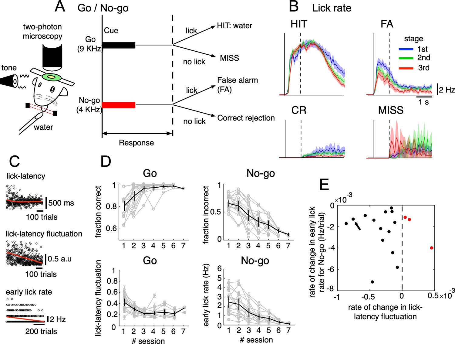
Go/No-go auditory-cue discrimination task and behavior changes during learning.
(A) Schematic diagram of a mouse performing the Go/No-go discrimination task under a two-photon microscope. (B) the lick rate of the four cue-response conditions sampled in the three learning stages (blue, green and red traces for 1st, 2nd, and 3rd stages, respectively). Thick lines and shadings represent mean ± s.e.m (n=12,334, 5,588, 7,681 and 914 trials for HIT, FA, CR and MISS, respectively). Solid and dashed vertical lines in A-B indicate the timing of cue onset and end of the response window, respectively. (C) from top to bottom, lick-latency, lick-latency fluctuation in Go trials and the early lick rate in No-go trials of a representative mouse (indicated by black arrow in E). Trials were sorted by the time course of training. Red traces indicate polynomial fittings of lick parameters as functions of trials (see Methods). (D) changes in four learning indices as functions of training sessions, including the fraction correct of Go cues, the fraction incorrect of No-go cues, lick-latency fluctuation in Go trials, and the early lick rate in No-go trials. Thin gray traces represent individual animals (n=17) and thick dark traces with error bars represent mean ± s.e.m across all animals. (E) scatterplot for rate of change in lick-latency fluctuation for Go cues (abscissa) and rate of change in early lick rate for No-go cues (ordinate) estimated from licking behavior of individual mice. Black dots were for mice whose rates were both negative and red dots were for the three mice that showed increased lick-latency fluctuation after learning (positive rate).
-
Figure 1—source data 1
Datasets used to create Figure 1.
- https://cdn.elifesciences.org/articles/86340/elife-86340-fig1-data1-v2.zip
Figure 1—figure supplement 1

Licking behavior in the early response window for individual mice.
Lick-latency (A) and lick-latency fluctuation (B) in HIT trials, early licks in No-go (CR and FA) trials (C), estimated from a window of 0–500ms after cue, of 17 mice. Trials were sorted by training session. Red traces in A-C indicated polynomial fits of the variables as the functions of trials (4th order for A and 1st order for B and C).
Figure 2 with 2 supplements
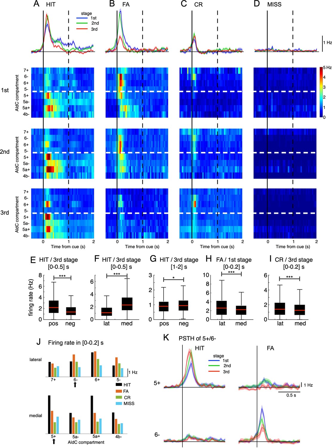
Opposite changes in CS firings in the lateral and medial parts of Crus II.
(A–D) Top row: population peri-stimulus time histograms (PSTHs) of CSs sampled for all recorded neurons (n=6,445) during three learning stages across four cue-response conditions: HIT trials (n=12,334, A), FA trials (n=5,588, B), CR trials (n=7,681, C), and MISS trials (n=914, D). From second to bottom rows: pseudo-color representation of PSTHs in each AldC compartment in Crus II sampled in three learning stages. Vertical black solid lines and black dashed lines represent the cue onset and the end of response window, respectively. Thick white dashed lines represent the boundary between lateral vs. medial hemispheres of Crus II. (E–I) Box plots show CS firing rate estimated for the AldC positive vs. negative compartments and lateral vs. medial Crus II in various configurations of the cue-response condition, learning stages and temporal windows. For each box plot, the black bar indicates the 25% and 75% and the central red mark indicates the median. Asterisks indicate the significance level of one-way ANOVA: * p<0.05, **** p<0.0001. (J) CS firing rate sampled in 0–0.2 s after cue onset for HIT (black bars), FA (orange bars), CR (green bars), and MISS (cyan bars) trials across all three learning stages for individual AldC compartments. Black arrows indicate the two representative AldC compartments that show the largest changes in CS activity after learning for HIT (5+) and FA (6-) trials. (K) PSTHs in HIT and FA trials of the two representative AldC compartments 5+ (n=1,117 and 575 for HIT and FA trials, respectively) and 6- (n=822 and 408 for HIT and FA trials, respectively) during learning. Thick lines and shadings in (A-D) and (K) represent mean ± s.e.m.
-
Figure 2—source data 1
Datasets used to create Figure 2.
- https://cdn.elifesciences.org/articles/86340/elife-86340-fig2-data1-v2.zip
Figure 2—figure supplement 1
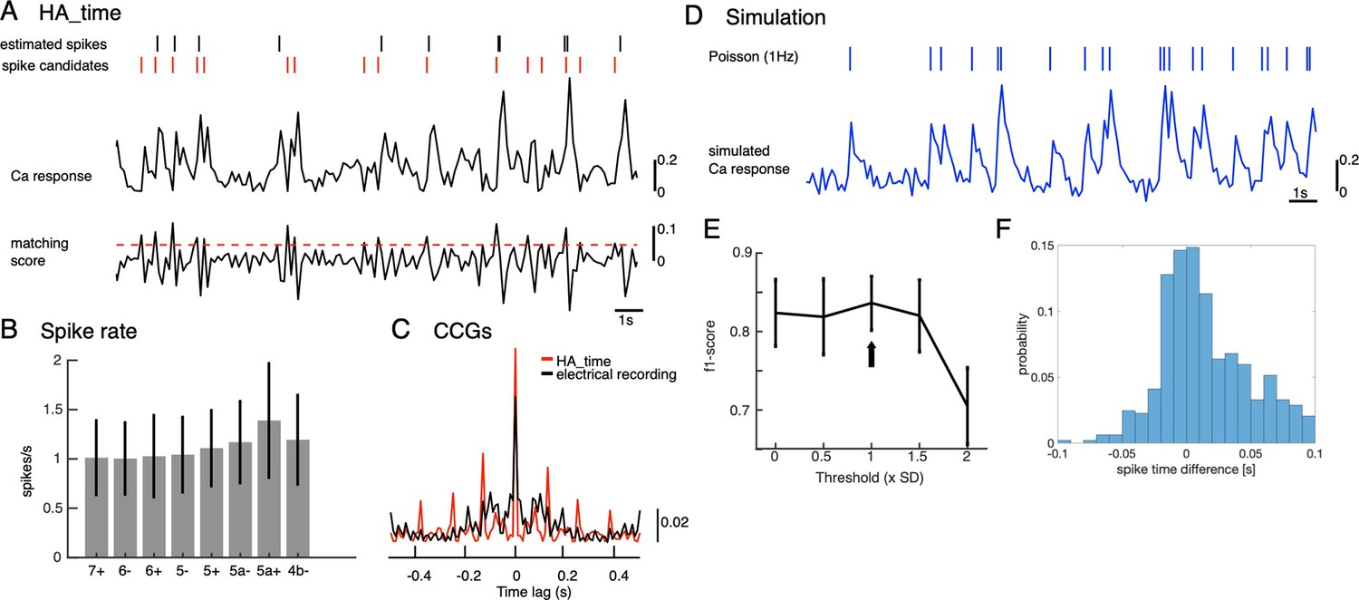
Illustration of CF reconstruction by HA_time and its examination.
(A) The spike model (inset) was estimated for Ca2+ signals (top trace) of two-photon recordings by Bayesian inference, assuming size and shape constancy of spikes. Spike candidates (red short bars) were selected by thresholding (threshold = 1 std, red dashed line) matching scores of Ca2+ signals (bottom trace) with the spike model, and spikes were selected by SVM from spike candidates. We optimized the threshold for matching score so as to maximize the F1-score so that it was >0.8 (black arrow, D). Finally, spike timings (black short bars) were estimated with temporal resolution of 100 Hz, so as to minimize residuals of observed and predicted Ca2+ signals by the model (Hoang et al., 2020b). (B) Spike rates of estimated CSs by HA_time across the AldC compartments. The mean firing rate (1.1±0.4 spikes/s) agrees with electrical recordings in behaving mice (Tsutsumi et al., 2020). (C) population CCG of spikes estimated by HA_time in a recording session of the AldC compartment 5+ (red histogram, n=20 cells) is consistent with that of multichannel electrical recording of Purkinje cells (black histogram, n=25 cells) reported in Blenkinsop and Lang, 2006. (D) Simulation of the Ca2+ signal (blue trace) was generated by convolution of the spike model and Poisson spikes (rate, 1 Hz, short blue bars), adding Gaussian noise (SNR = 10). (E–F) f1-score (E) and spike time difference between true and estimated spikes (F) by HA_time with the threshold values varied from 0 to 2 std in spike candidate selection. Simulated Ca2+ signals of a total of five Purkinje cells indicated that HA_time was capable of detecting roughly 90% of the spikes with mean spike time difference of about 30ms.
Figure 2—figure supplement 2

Synchrony dynamics and associated synchrony-response bidirectional changes in AldC compartments 5+and 6-.
(A) Synchrony analysis of representative sessions for 5+/HIT and 6-/FA trials. Upper: snapshots of synchronous firings in HIT trials at the boundary 5+/5- of two representative sessions in 1st and 3rd stages. Reference cells (black arrows) are those that show the largest difference in HIT-FA responses. Stair-plots indicate CCGs between the reference cell and the proximal cell (open arrows) that has the highest pairwise synchrony strength in the session. Lower: similar plots of representative sessions for 6-/FA trials. (B) Population CCGs for all sampled cell pairs in 5+/HIT (upper) and 6-/FA trials (lower) for the 1st and 3rd stages. Red traces in CCGs indicate shift predictors estimated for the correlation solely to cue stimuli. (C) Scatterplots of averaged spike counts and instantaneous synchrony across all trials, both estimated in the window of 300ms before the first lick, for HIT (left column) and FA (right column) trials in three stages of learning for two representative AldC compartments 5+ (upper row, n=1,117 and 575 for HIT and FA trials, respectively) and 6- (lower row, n=822 and 408 for HIT and FA trials, respectively). Thick black trace indicates correlation of the two quantities. Summary statistics of instantaneous synchrony and spike count were shown by horizontal and vertical box plots, respectively. For each box plot, the bar indicates the 25% and 75% and the central mark indicates the median. The whiskers extend to the most extreme data points not considered outliers. Asterisks indicate significant level of one-way ANOVA: n.s, p>0.05; * p<0.05; **** p<0.0001.
Figure 3 with 1 supplement
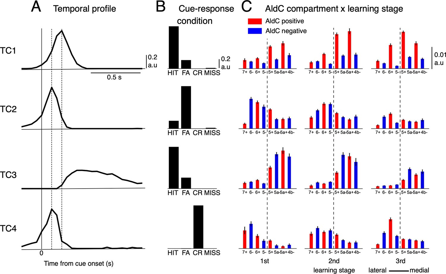
Tensor component analysis of CS activity.
(A–C) (A) Coefficients of temporal, (B) cue-response condition, and (C) neuronal factor of the four tensor components (TC1-TC4, from top to bottom) estimated by TCA. TCs are shown in their contribution order (see Methods for details). The three vertical lines in (A) represent the timing at 0, 100 and 200ms after the cue onset. Bars with lines in (C) show means and SDs of neuron factor coefficients, grouped by eight AldC compartments (shown in red and blue colors for AldC positive and negative compartments, respectively) and three learning stages (n=6,445 neurons). The thick dashed line in (C) indicates a functional boundary between the lateral and medial Crus II (Tsutsumi et al., 2019).
-
Figure 3—source data 1
Datasets used to create Figure 3.
- https://cdn.elifesciences.org/articles/86340/elife-86340-fig3-data1-v2.zip
Figure 3—figure supplement 1
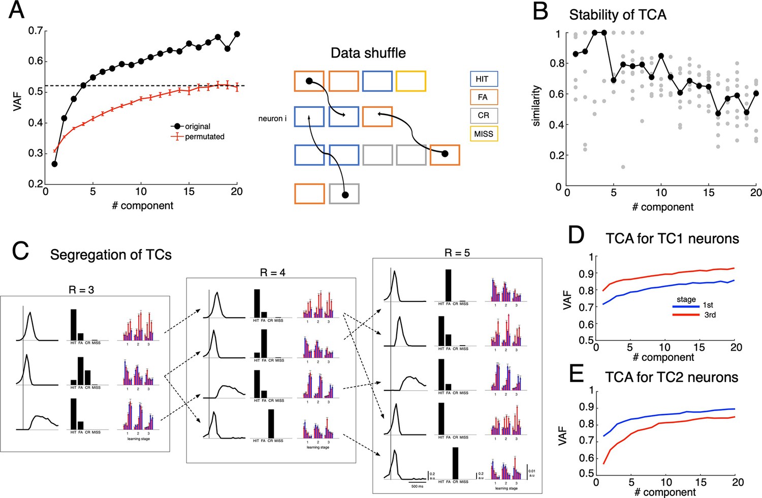
Tensor component analysis of population PSTHs with a varied number of tensor components and the permutation test.
(A) The fitting performance of TCA, which estimates variance accounted for (VAF) of the reconstructed data using optimal solutions (see Methods for details), with the number of tensor components varied from R=1–20 (left). The dashed black line indicates values at R=4, which explains approximately 50% of variance. Similar TCA was applied to data with spiking activity shuffled among neurons and trials (see right panel for schematic of data shuffle and Methods for details). The shuffle was conducted for n = 100 random permutations (red line indicates mean and error bars as s.e.m of VAF values). (B) Similarity scores, which measure the similarity between solutions of n=10 random initializations (gray dots) with the optimal solution, for each of the number of tensor components R. The black dots represent the median of similarity scores. (C) Optimal TCA solutions for R=3, 4, 5 showed the segregation of TCs while increasing R. Dashed arrows were drawn by visual inspection of the similarity in temporal profile, cue-response condition and zonal distribution, between the TCs. (D-E): TCA for the top 300 TC1 (D) and TC2 neurons (E) at the first (blue traces) and third (red traces) learning stages showed an opposite change in dimensionality of TC1-2 after learning (i.e. the dimensionality decreased for TC1 and increased for TC2).
Figure 4 with 2 supplements
Dynamics of synchrony and opposite changes in synchrony of TC1-TC2 neurons during the course of learning.
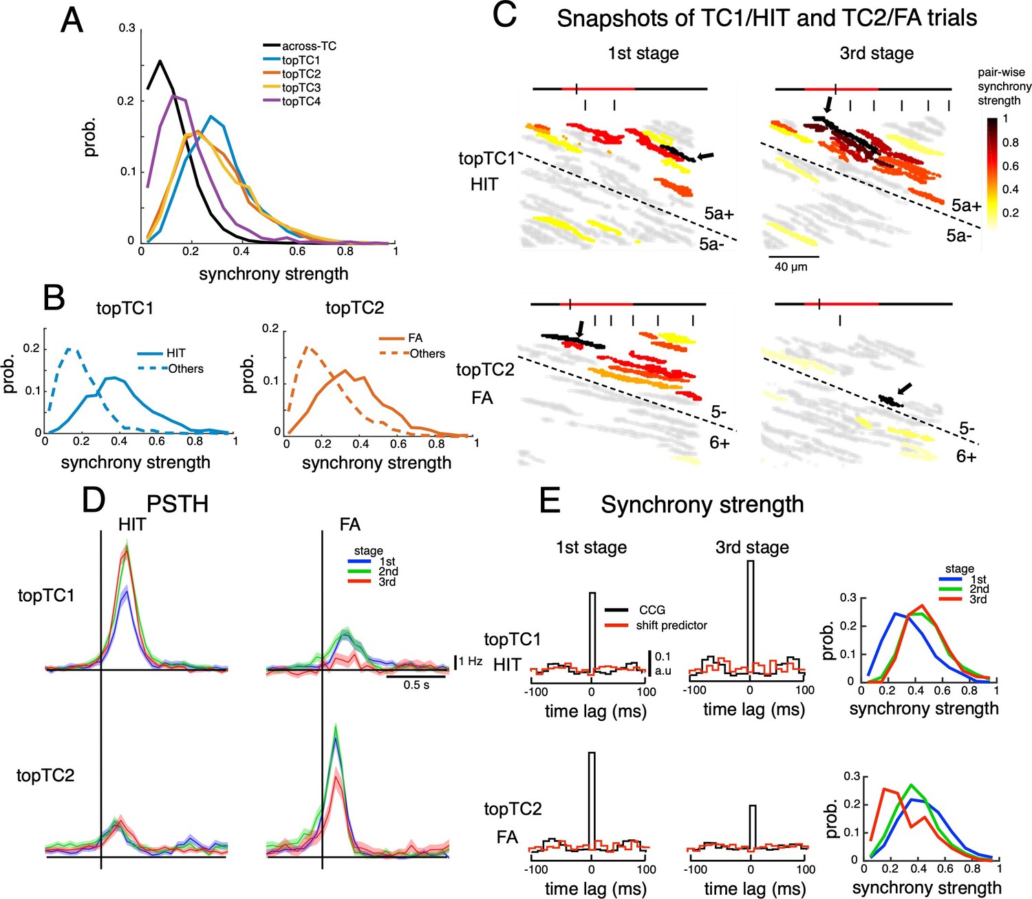
(A) Histograms of synchrony strength between topTC1-4 neurons (colored traces, n=508, 461, 581 and 546 for topTC1-4, respectively) in comparison with those across TCs (black trace). (B) Histograms of synchrony strength computed specifically in HIT trials for topTC1 neurons (solid blue trace) and in FA trials for topTC2 neurons (solid orange trace), contrasting with those in other cue-response conditions (dashed traces). (C) Representative images of synchronous firings in TC1/HIT (5a-/5a+) and TC2/FA (6+/5-) in the 1st and 3rd stages. The horizontal line shows the time course of –200ms to 1 s after cue onset with a small tick indicating the timing of the snapshot relative to the cue onset (the cue period of 500ms was shown in red color). Short vertical bars indicate lick timings. Snapshots capture responses of Purkinje cell dendrites (gray areas) co-activated in a time bin of 10ms. The hot-color spectrum represents pair-wise synchrony strength between reference cells (pointed by black arrows) and other cells in the same recording session (see Video 1). (D) PSTHs of topTC1-TC2 neurons in HIT (n=1,983 and 1,703 for topTC1 and topTC2, respectively) and FA (n=1,010 and 813 for topTC1 and topTC2, respectively) trials in three learning stages. (E) Population cross-correlograms (CCGs) of the 1st and 3rd stages indicated opposite changes in synchrony strength of topTC1-TC2 neurons during learning. Red traces in CCGs indicate shift predictors estimated for the correlation solely due to the cue stimulus. Solid lines in the right panels represent histograms of synchrony strength within topTC1 and topTC2 neurons in HIT and FA trials, respectively, for the three learning stages.
-
Figure 4—source data 1
Datasets used to create Figure 4.
- https://cdn.elifesciences.org/articles/86340/elife-86340-fig4-data1-v2.zip
Figure 4—figure supplement 1
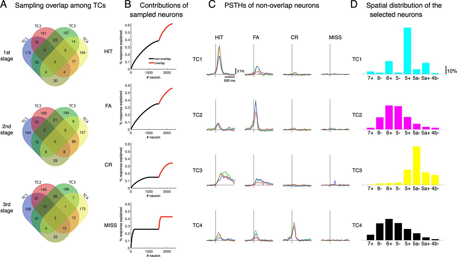
Neural sampling by TCA.
(A) At each learning stage, we sampled 300 neurons whose coefficients were highest for each of the tensor components, TC1-4. The Venn diagram shows the number of overlapping neurons by this sampling. We excluded overlapping neurons from further analysis in the main results. (B) The response explained was estimated by the ratio of accumulated responses of sampled neurons for 1 s after cue onset to the accumulated response of a total of 6,445 neurons. Black and red are for selected neurons without overlapping ones and overlapping neurons. (C) PSTHs in the four cue-response conditions of topTC neurons without overlapping neurons. (D) Spatial distribution of the selected topTC1-4 neurons.
Figure 4—figure supplement 2
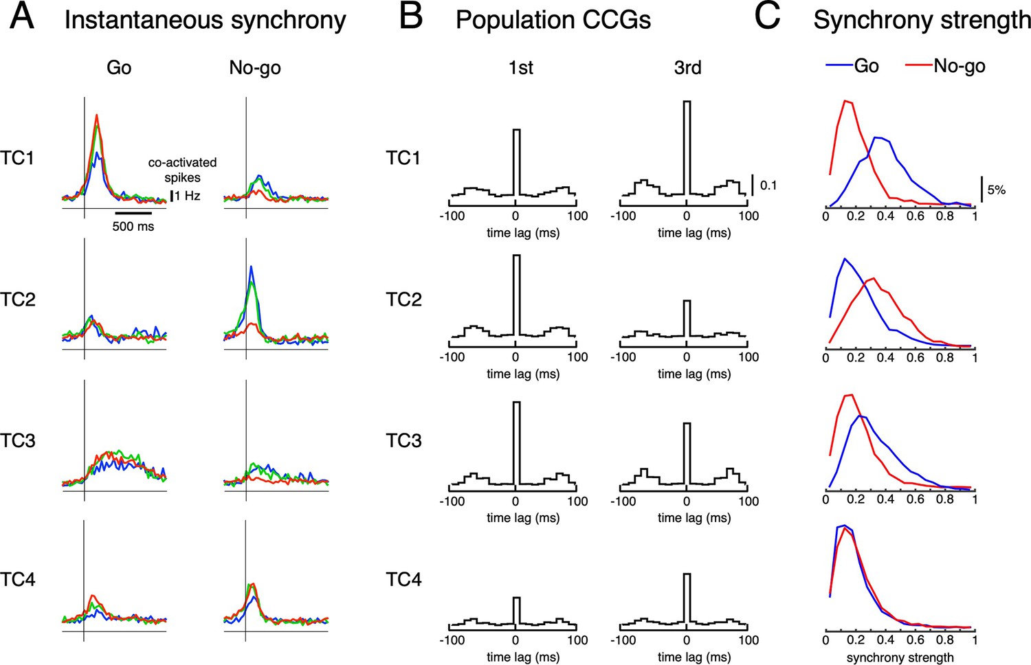
Synchronous firings of TCs.
(A) Averaged number of co-activated neurons following Go and No-go cues of the four TCs. Averaged instantaneous synchrony across trials. (B) Population CCGs of sampled topTC neurons in the 1st (first column) and 3rd (second column) learning stages. (C) Histograms of synchrony strength of topTC neurons for Go (blue) and No-go (red) cues. These results indicate that synchrony was high in cue-response conditions that are maximally associated with TC activities.
Figure 5 with 5 supplements
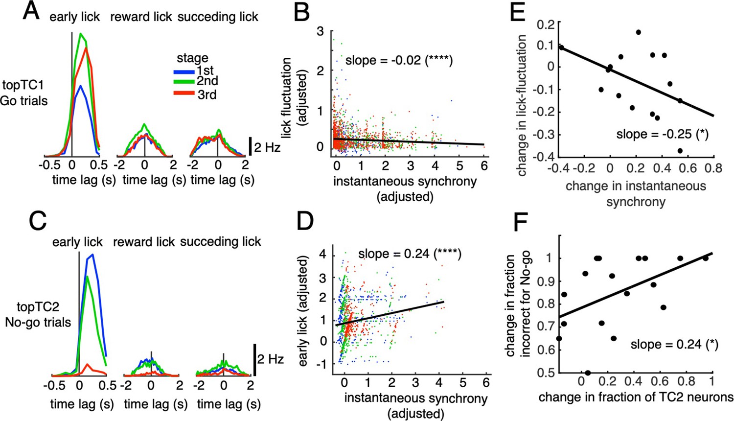
Correlations between synchronous activities in TC1-2 neurons and licking behavior.
(A) Synchronous CS-triggered lick responses of topTC1 neurons in the three response windows: early lick (0–0.5 s after cue onset), reward lick (0.5–2 s) and succeeding lick (2–4 s). (B) Scatterplot of instantaneous synchrony and lick-latency fluctuation in Go trials (n=2,115) of topTC1 neurons. (C) Synchronous spike-triggered lick responses of topTC2 neurons in the three response windows similar to those in A. (D) Scatterplot of instantaneous synchrony and number of early licks in No-go trials (n=965) of topTC2 neurons. Each dot in scatterplots of B-D corresponds to a single trial. We used a multiple linear regression model with the two learning variables as functions of instantaneous synchrony of the four topTCs and fraction correct. The black trace represents the correlation of two learning variables and instantaneous synchrony, with a slope and significance level indicated by asterisks. Note that the ordinate and abscissa of scatterplots in A-B were adjusted to show correlations specific to topTC1 or topTC2 neurons (see Methods). (E) The scatter showed correlation of the amount of change in instantaneous synchrony of TC1 neurons (abscissa) and amount of change in lick-latency fluctuation (ordinate) across n=17 mice. For individual mice, the amount of change was computed as differences between sessions that have the highest and lowest fraction correct for Go cues. Each black dot represents a single animal. (F) Plot similar to E, but for the amount of change in fraction of TC2 neurons (abscissa) and amount of change in fraction incorrect for No-go cues (ordinate). The amount of changes was computed as differences between sessions that have the highest and lowest fraction incorrect for No-go cues.
-
Figure 5—source data 1
Datasets used to create Figure 5.
- https://cdn.elifesciences.org/articles/86340/elife-86340-fig5-data1-v2.zip
Figure 5—figure supplement 1
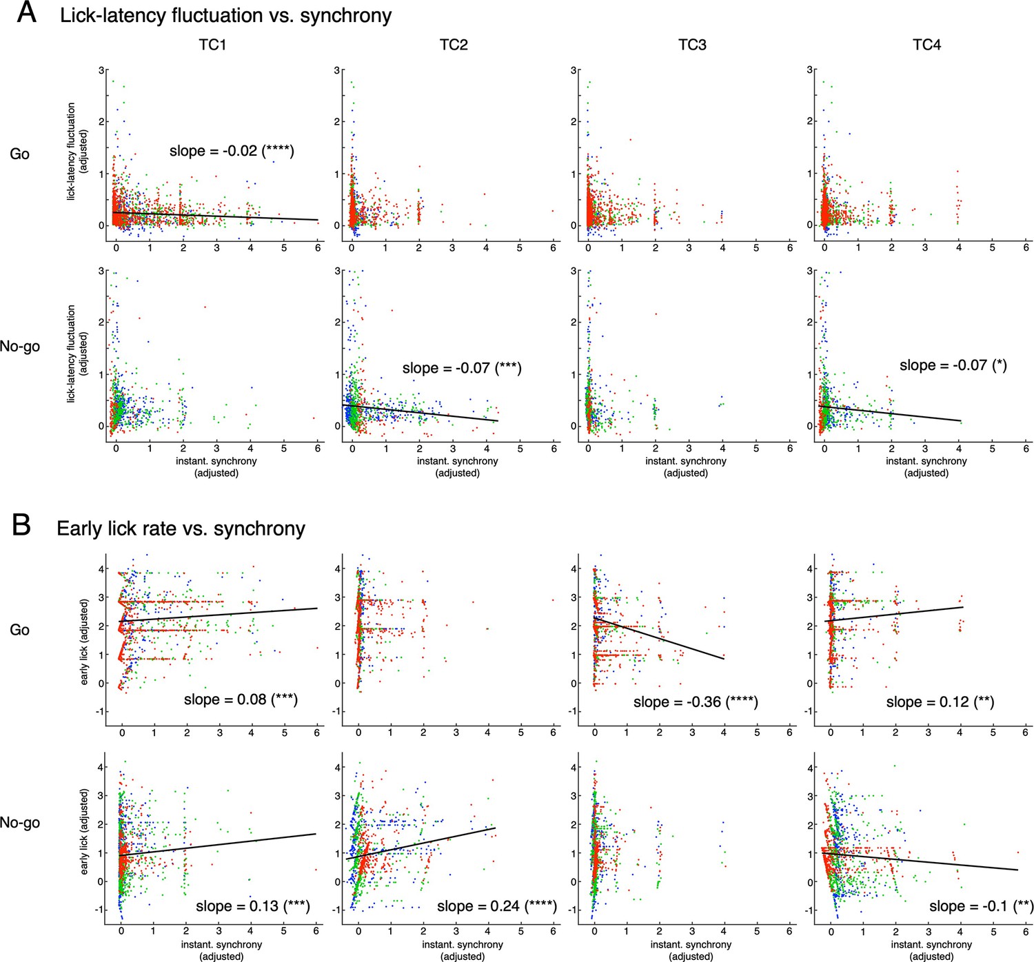
Multiple regression analysis for two lick variables (lick-latency fluctuation and early lick rate) and synchrony of topTC1-4 neurons.
The top and bottom rows in A and B are for Go and No-go cues, respectively. The four columns are for TC1 – TC4. Only significant correlations (p<0.05) are shown by black lines with slope values. The ordinate and abscissa were adjusted to show partial correlations of lick variable and synchrony of single TCs (see Methods for more details). Note that slopes for fraction correct variable were all significant (p<0.0001), but negative for lick-latency fluctuation/Go (top row in A) and early-lick-rate/No-go (bottom row in B) and positive for lick-latency fluctuation/No-go (bottom row in A) and early-lick-rate/Go (top row in B) combinations. These results are consistent with behavioral results that there was no learning in reduction of lick-latency fluctuation for No-go trials or early lick rate for Go trials.
Figure 5—figure supplement 2
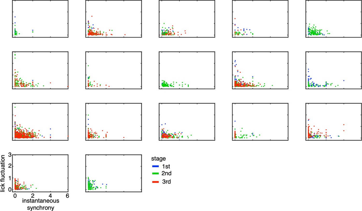
Lick-latency fluctuation in Go trials as a function of instantaneous synchrony in TC1 neurons for individual animals.
The scatters indicated lick-latency fluctuation for Go trials (ordinate) and instantaneous synchrony estimated among TC1 neurons in the same recording session (abscissa). Each dot represents a single trial (blue, green and red for 1st, 2nd, and 3rd stages, respectively). Each panel corresponds to a single animal.
Figure 5—figure supplement 3
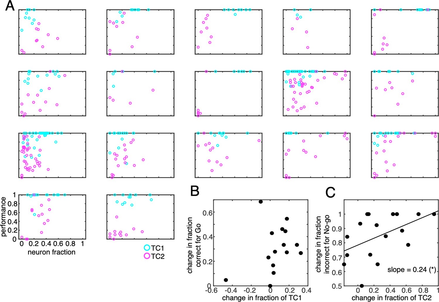
Behavioral performance as a function of neuron fraction for individual animals.
(A) Fraction correct for Go (=HIT/HIT + MISS) and fraction incorrect for No-go (=FA/FA + CR) cues were plotted as a function of the fraction of TC1 (cyan circles) and TC2 (magenta circles) neurons in each of the recording session, respectively. Each panel corresponds to a single animal. Each dot represents a session. (B) the scatter plots changes in fraction of TC1 neurons (abscissa) and changes in fraction correct for Go cues for 17 mice. Each dot represents a single animal. (C) Similar to B but for changes in fraction of TC2 neurons and fraction incorrect for No-go cues. (C) was reported in the main text as Figure 5F.
Figure 5—figure supplement 4

Decoding analysis of lick events.
(A) Spike-triggered lick response for all spike and lick events sampled from 0 to 1 s after the cue onset in HIT and FA trials. (B) Likelihood estimation of a lick given different kinds of spike events in a representative HIT trial. Spike events were sampled according to the three spiking models, including synchronous spikes of topTC1 neurons (blue), all spikes of topTC1 neurons (orange), and all spikes of all neurons in the same recording session (yellow). Note that 0.01 indicates the chance level (black) to correctly predict the occurrence of a single lick at 100 Hz precision. Black dots indicate licking events. (C) For each single lick event, the best model was determined for the maximal likelihood among the four models. Pie charts indicated the percentage of the best model for the entire TC1/HIT (left) and TC2/FA (right) trials.
Figure 5—figure supplement 5

Effect of muscimol injection on lick timing precision.
(A) Lick-latency in HIT trials for saline (left) and muscimol (right) conditions of 5 animals. Red traces showed 4th order polynomial fits of the lick-latency as functions of trials. (B) Increases of mean lick-latency fluctuation (ordinate, see Methods for more details) in 4 out of 5 animals indicated that muscimol effectively reduced precision of lick timing compared with saline conditions.
Figure 6 with 2 supplements
Tensor representation of individual Purkinje cells in Crus II.
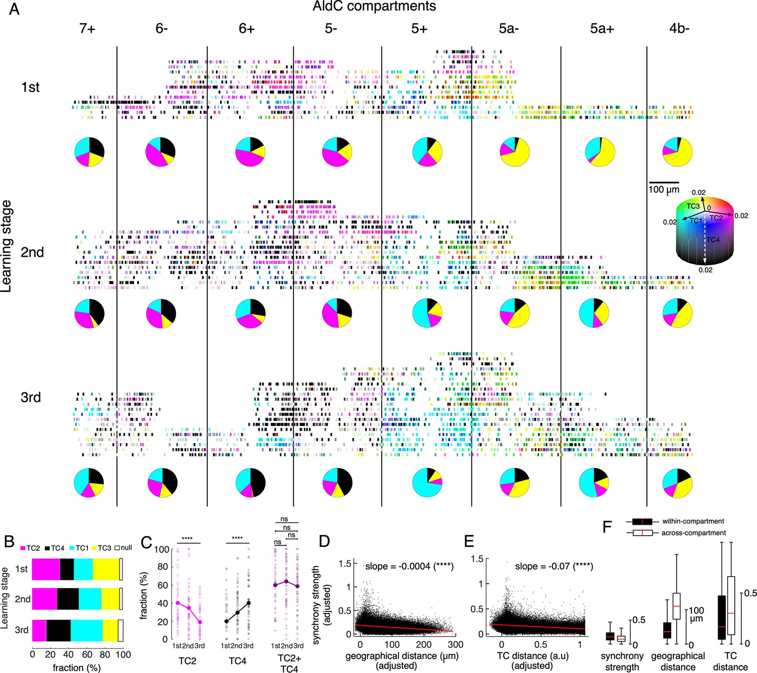
(A) CS firing in n=6,465 neurons in 8 AldC compartments (columns) and at three learning stages (rows) were evaluated by TCA. Each short bar indicated the location of a single cell relative to the AldC boundaries (vertical black lines). The color of each cell was mixed by coefficients of the four TCs (cyan – TC1, magenta – TC2, yellow – TC3 and black – TC4). Each row corresponds to a single recording session. For visualization purposes, the width of each AldC compartments was manually adjusted to 300 μm. Pie-charts indicate fraction of TC1-4 neurons in each AldC compartment and at each learning stage. (B) Fractions of neurons classified as TC1-4 in each of the three learning stages (color bars). Note that less than 6% of all recorded neurons could not be classified as TC1-4 (null, open bars). (C) Fractions of neurons in the lateral Crus II (AldC compartments 7+, 6-, 6+, 5-) classified as TC2 (magenta) and TC4 (black) and their summation (TC2 + TC4, dark magenta) in n=150 sessions (small open circles) and their means (solid large circles) for the three learning stages. (D–E) Correlations between the synchrony strength vs. geographical distance (D), synchrony strength vs. TC distance (E). A single black dot corresponds to a neuronal pair (n=170,396 pairs). The red line represents the correlation between measures with a slope and significance level indicated by asterisks. Note that the ordinate and abscissa of scatterplots in D-E were adjusted to show correlations specific to geographic distance or TC distance between neuron pairs, similar to the multiple regression analysis performed in Figure 5B&D. (F) Box plots show the three measures sampled for within-compartment (filled boxes, n=87,192 pairs) and across-compartment groups (open boxes, n=83,204 pairs). Description of the box plot is the same as in Figure 2E–I.
-
Figure 6—source data 1
Datasets used to create Figure 6.
- https://cdn.elifesciences.org/articles/86340/elife-86340-fig6-data1-v2.zip
Figure 6—figure supplement 1

PCA of Go/No-go data.
(A) Schematic of the input vector for TCA and PCA, in which cue-response conditions were concatenated for single neurons. Lower panel shows the VAF profile of PCA. (B) Scatter of the first two principal components with colors representing the selected topTC1-4 neurons (cyan, magenta, yellow and black circles, respectively), and the remaining neurons as gray circles. k-mean clustering using PC scatters of the topTC1-4 neurons show consistent result with neuronal classification by TCA (i.e, topTC1 neurons ~cluster #2, topTC2 neurons ~cluster #4, topTC3 neurons ~cluster #1, and topTC4 neurons ~cluster #3 and #4). (C) PCA at the level of trial-averaged (orange line) and single-trial (blue line) showed comparable VAF profiles. (D) Correlation of PSTH between TC1 and TC2 neurons in HIT and FA trials, respectively. Here, the topTC1 and topTC2 neurons were sampled across all learning stages, and further divided into 2 groups of ‘within-zone’ (dark blue columns) and ‘across-zone’ (light blue columns). The baseline was computed for all recorded neurons (gray columns). Bars with errors indicate means and standard deviations.
Figure 6—figure supplement 2
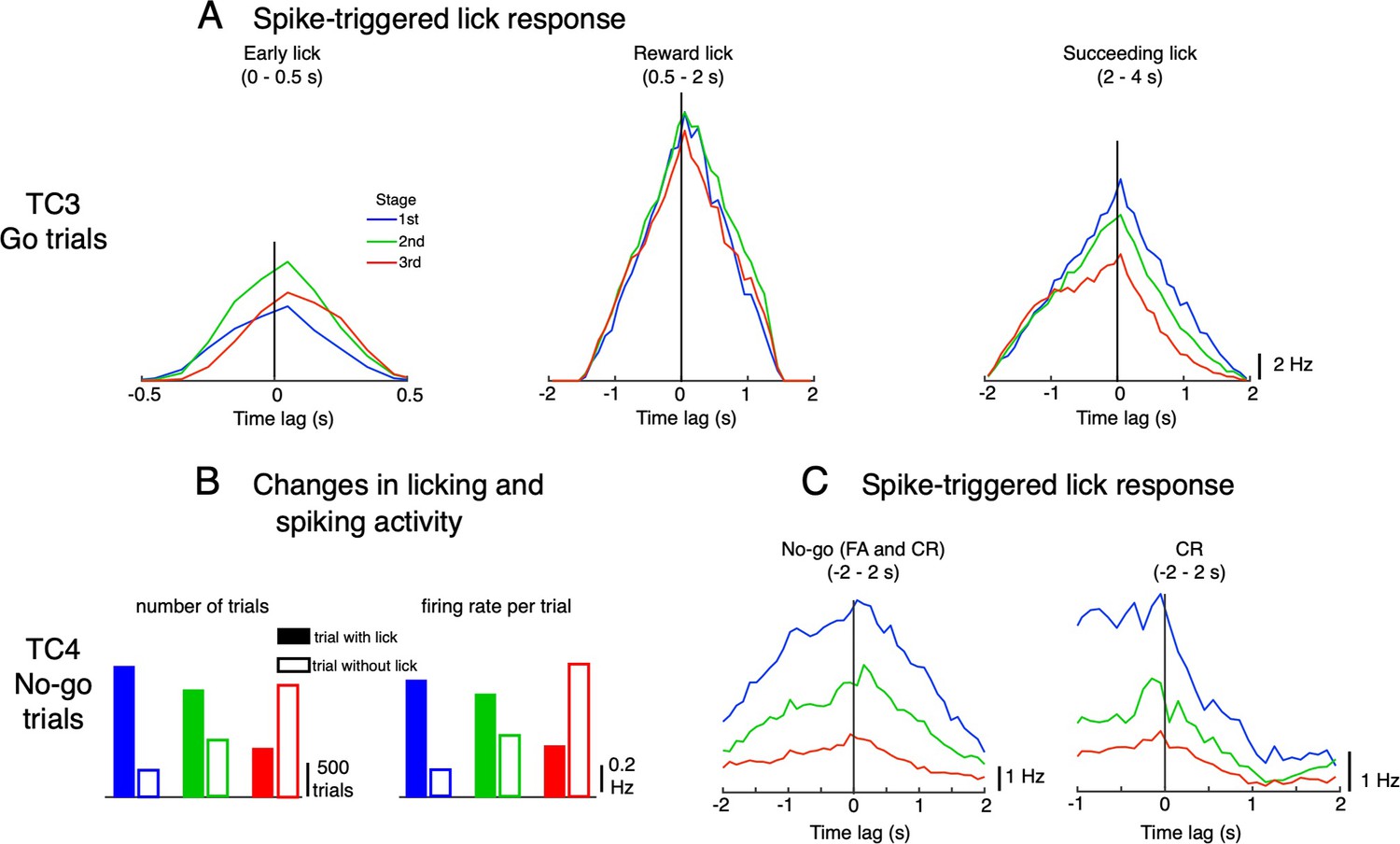
Possible functions of TC3 and TC4.
(A) Spike-triggered lick response for topTC3 neurons for Go trials in the three response windows: early lick (0–0.5 s), reward lick (0.5–2 s) and succeeding lick (2–4 s). Lick responses were largest for the reward window with a balanced distribution of negative-positive values, suggesting that TC3 is equally related to sensory feedback and motor control of reward licks. (B) Change in numbers of trials with (filled bars) and without licks (open bars) during learning, and mean firing rate per trial of topTC4 neurons for No-go cues. (C) Spike-triggered lick responses of topTC4 neurons plotted for No-go cues (including FA and CR trials, left) and separately for CR trials (right) in the window –2–2 s after cue. Note that according to the experimental design, the subsequent trial was delayed by 1 s from the last lick if the mouse continued to lick. Thus, to compute the spike-triggered lick response of TC4 in –2–2 s of No-go trials, the transition period of –1–0 s, during which there were no licks, was ignored.
Author response image 1

Synchrony strength of TC1 (cyan crosses) and TC2 (magenta crosses) neurons as function of fraction correct for Go cues (cyan lines) and fraction incorrect for No-go cues (magenta lines), respectively.
Each panel corresponds to a single animal. The scatter at the lower-right panel showed the rate of change (i.e. the slope of synchrony strength vs. performance) in TC1 synchronization (abscissa) and the rate of change in TC2 synchronization (ordinate) of 17 animals. Each black dot represents a single animal.
Videos
Video 1
CF firings in 10 ms bins of Ald-C compartment 5+neurons for HIT trials in two representative sessions of the 1st and 3rd learning stages.
Detailed description for the elements can be found in Figure 4C.
Video 2
Relationship of TC coefficient, synchrony strength and instantaneous synchrony within individual Ald-C compartment for HIT trials in the 1st and 3rd learning stages of TC1.
For each Ald-C compartment (column), the neuron which has highest TC1 coefficients (bottom row) was selected as a reference neuron. Instantaneous synchrony in a single trial (top row) and synchrony strength (second row) were estimated between the reference neuron and other neurons in the same compartment. While synchrony strength was static within session, instantaneous synchrony varies trial-to-trial with strong values observed for HIT trials but not trials of the other cue-response conditions.
Additional files
-
Supplementary file 1
Summary of two-photon recordings.
(a) The number of PCs sampled in individual AldC compartments at different learning stages. (b) The number of trials for each cue-response condition at different learning stages.
- https://cdn.elifesciences.org/articles/86340/elife-86340-supp1-v2.docx
-
MDAR checklist
- https://cdn.elifesciences.org/articles/86340/elife-86340-mdarchecklist1-v2.docx
Download links
A two-part list of links to download the article, or parts of the article, in various formats.
Downloads (link to download the article as PDF)
Open citations (links to open the citations from this article in various online reference manager services)
Cite this article (links to download the citations from this article in formats compatible with various reference manager tools)
Dynamic organization of cerebellar climbing fiber response and synchrony in multiple functional components reduces dimensions for reinforcement learning
eLife 12:e86340.
https://doi.org/10.7554/eLife.86340


