BrainPy, a flexible, integrative, efficient, and extensible framework for general-purpose brain dynamics programming
- School of Psychological and Cognitive Sciences, IDG/McGovern Institute for Brain Research, Peking-Tsinghua Center for Life Sciences, Center of Quantitative Biology, Academy for Advanced Interdisciplinary Studies, Bejing Key Laboratory of Behavior and Mental Health, Peking University, China
- Guangdong Institute of Intelligence Science and Technology, China
- Beijing Jiaotong University, China
Figures
Figure 1
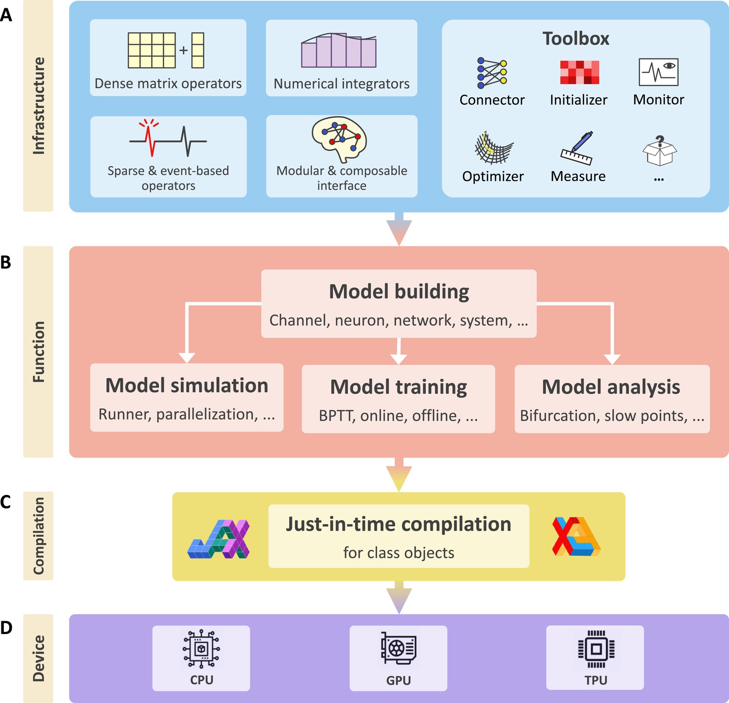
BrainPy is an integrative framework targeting general-purpose brain dynamics programming.
(A) Infrastructure: BrainPy provides infrastructure tailored for brain dynamics programming, including NumPy-like operators for computations based on dense matrices, sparse and event-based operators for event-driven computations, numerical integrators for solving diverse differential equations, the modular and composable programming interface for universal model building, and a toolbox useful for brain dynamics modeling. (B) Function: BrainPy provides an integrated platform for studying brain dynamics, including model building, simulation, training, and analysis. Models defined in BrainPy can be used for simulation, training, and analysis jointly. (C) Compilation: Based on JAX (Frostig et al., 2018) and XLA (Sabne, 2020), BrainPy provides just-in-time (JIT) compilation for Python class objects. All models defined in BrainPy can be JIT compiled into machine codes to achieve high-running performance. (D) Device: The same BrainPy model can run on different devices including Central Processing Unit (CPU), Graphics Processing Unit (GPU), or Tensor Processing Unit (TPU), without additional code modification.
Figure 2
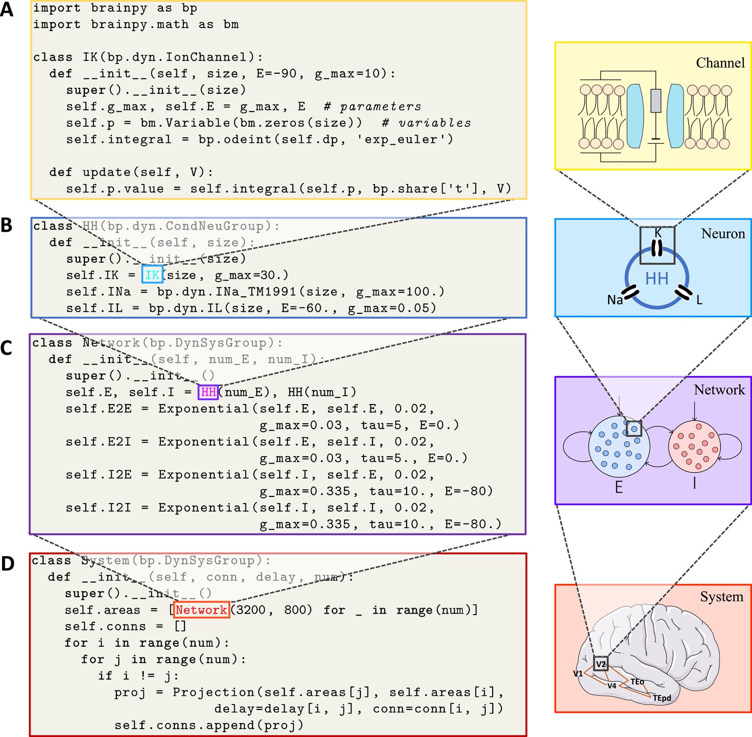
BrainPy supports modular and composable programming for building hierarchical brain dynamics models.
(A) An ion channel model is defined as a subclass of brainpy.dynz.IonChannel. The __init__() function specifies the parameters and states, while the update() function defines the updating rule for the states. (B) An Hodgkin–Huxley (HH)-typed neuron model is defined by combining multiple ion channel models as a subclass of brainpy.dyn.CondNeuGroup. (C) An E/I balanced network model is defined by combining two neuron populations and their connections as a subclass of brainpy.DynSysGroup. (D) A ventral visual system model is defined by combining several networks, including V1, V2, V4, TEo, and TEpd, as a subclass of brainpy.DynSysGroup. For detailed mathematical information about the complete model, please refer to Appendix 9.
Figure 3
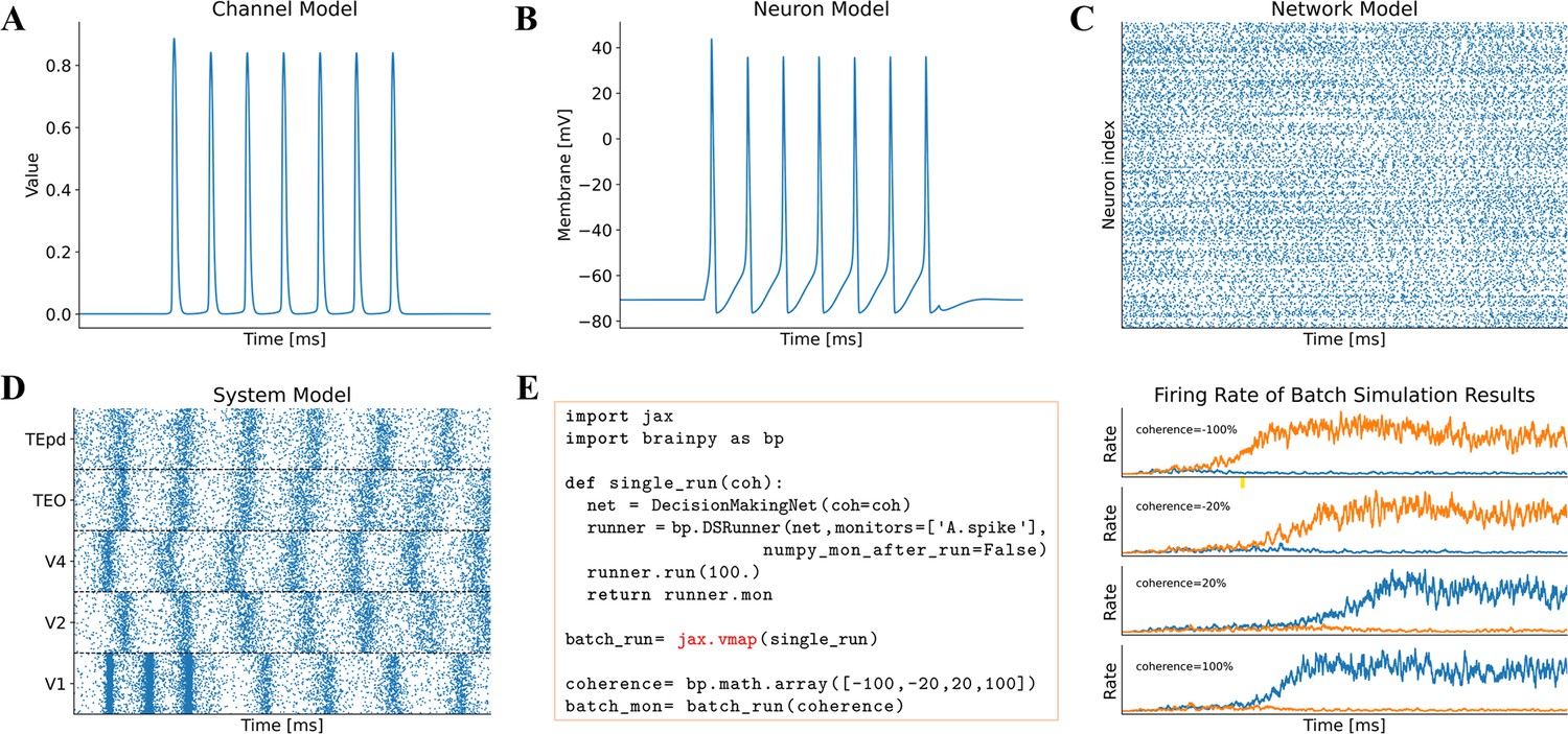
Model simulation in BrainPy.
The interface DSRunner supports the simulation of brain dynamics models at various levels. (A) The simulation of the potassium channel in Figure 2A. (B) The simulation of the HH neuron model in Figure 2B. (C) The simulation of the E/I balanced network, COBAHH (Brette et al., 2007) in Figure 2C. (D) The simulation of the ventral visual system model (the code please see Figure 2D, and the model please see Appendix 9). (E) Using jax.vmap to run a batch of spiking decision-making models (Wang, 2002) with inputs of different coherence levels. The left panel shows the code used for batch simulations of different inputs, and the right panel illustrates the firing rates under different inputs.
Figure 4
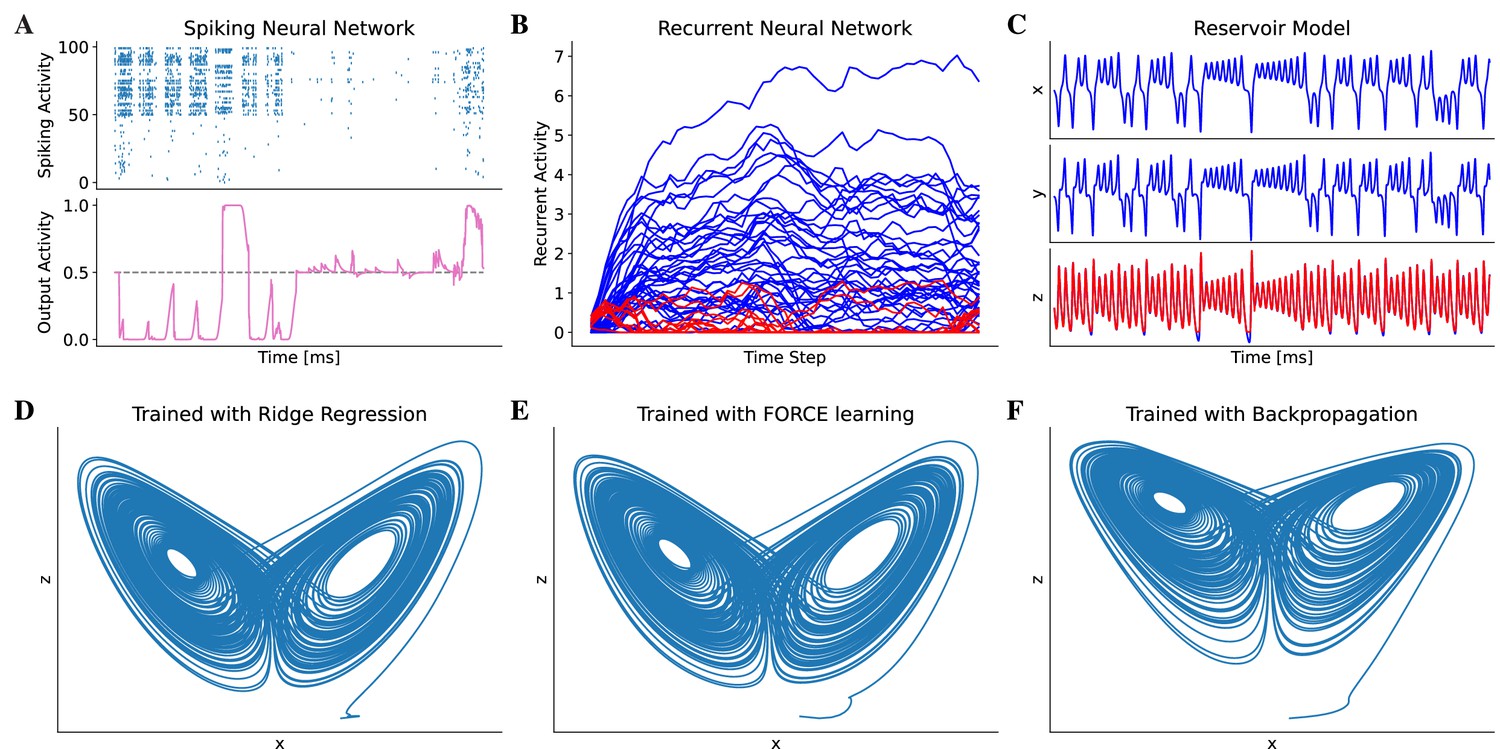
Model training in BrainPy.
BrainPy supports the training of brain dynamics models from data or tasks. (A) Training a spiking neural network (Bellec et al., 2020) on an evidence accumulation task (Morcos and Harvey, 2016) using the backpropagation algorithm with brainpy.BPTT. (B) Training an artificial recurrent neural network model (Song et al., 2016) on a perceptual decision-making task (Britten et al., 1992) with brainpy.BPTT. (C) Training a reservoir computing model (Gauthier et al., 2021) to infer the Lorenz dynamics with the ridge regression algorithm implemented in brainpy.OfflineTrainer. , and are variables in the Lorenz system. (D–F) The classical echo state machine (Jaeger, 2007) has been trained using multiple algorithms to predict the chaotic Lorenz dynamics. The algorithms utilized include ridge regression (D), FORCE learning (E), and backpropagation algorithms (F) implemented in BrainPy. The mean squared errors between the predicted and actual Lorenz dynamics were 0.001057 for ridge regression, 0.171304 for FORCE learning, and 1.276112 for backpropagation. Please refer to Appendix 10 for the training details.
Figure 5
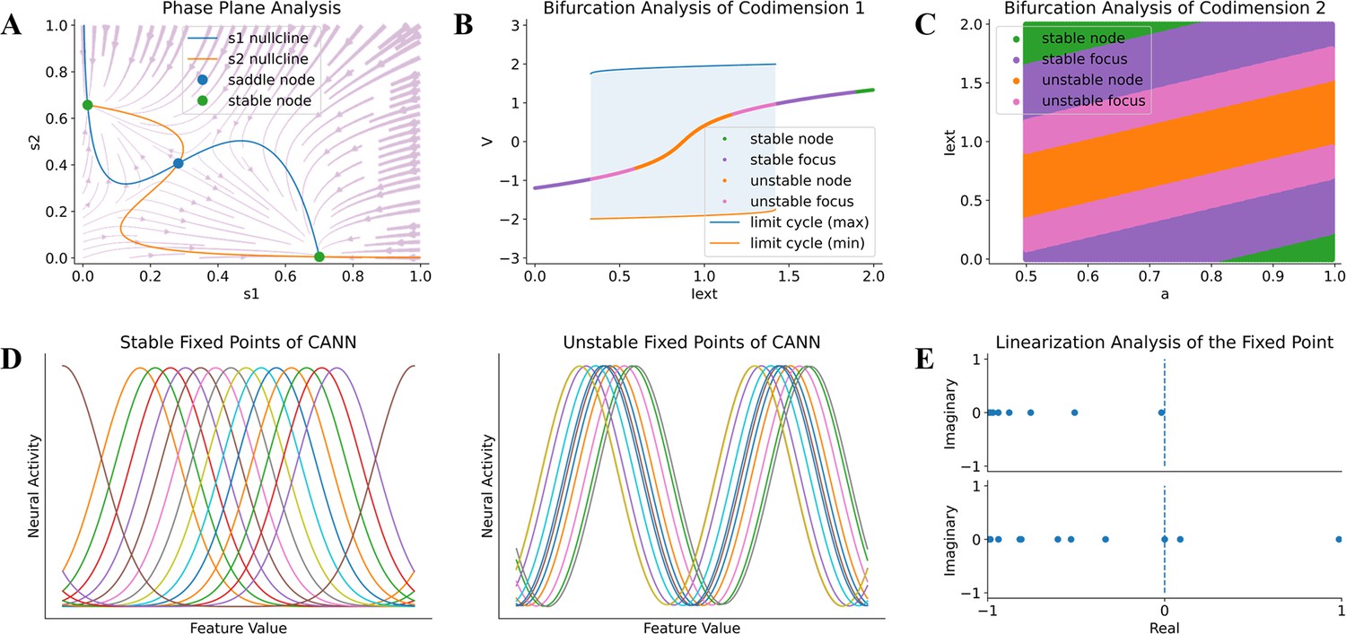
Model analysis in BrainPy.
BrainPy supports automatic dynamics analysis for low- and high-dimensional systems. (A) Phase plane analysis of a rate-based decision-making model (Wong and Wang, 2006). (B) Bifurcation analysis of codimension 1 of the FitzHugh–Nagumo model (Fitzhugh, 1961), in which the bifurcation parameter is the external input Iext. (C) Bifurcation analysis of codimension 2 of the FitzHugh–Nagumo model (Fitzhugh, 1961), in which two bifurcation parameters Iext and a are continuously varying. (D) Finding stable and unstable fixed points of a high-dimensional CANN model (Wu et al., 2008). (E) Linearization analysis of the high-dimensional CANN model (Wu et al., 2008) around one stable and one unstable fixed point.
Figure 6
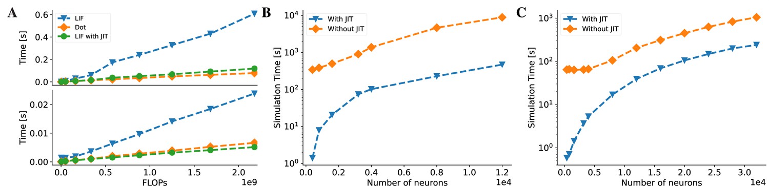
BrainPy accelerates the running speed of brain dynamics models through just-in-time (JIT) compilation.
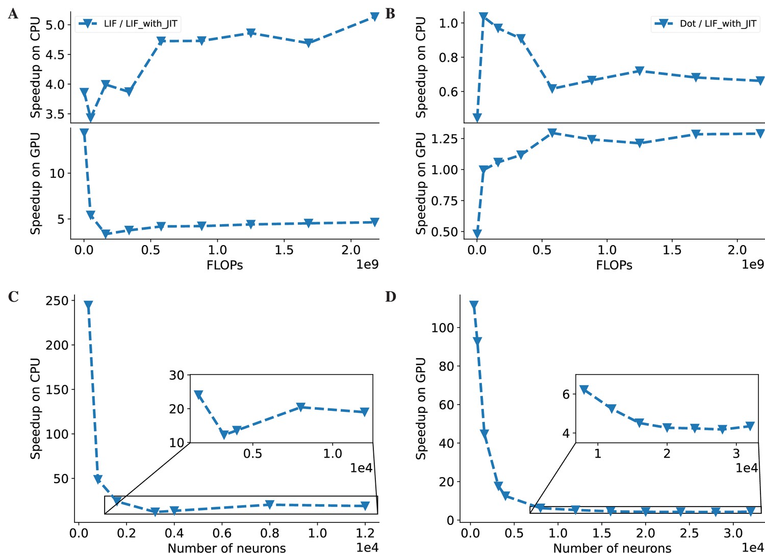
(A) Performance comparison between an LIF neuron model (Abbott, 1999) and a matrix–vector multiplication ( and ). By adjusting the number of LIF neurons in a network and the dimension in the matrix–vector multiplication, we compare two models under the same floating-point operations (FLOPs). The top panel: On the Central Processing Unit (CPU) device, the LIF model without JIT compilation (the ‘LIF’ line) shows much slower performance than the matrix–vector multiplication (the ‘Dot’ line). After compiling the whole LIF network into the CPU device through JIT compilation (the ‘LIF with JIT’ line), two models show comparable running speeds (please refer to Appendix 11—figure 6A for the time ratio). The bottom panel: On the Graphics Processing Unit (GPU) device, the LIF model without JIT shows several times slower than the matrix–vector multiplication under the same FLOPs. After applying the JIT compilation, the jitted LIF model shows comparable performance to the matrix–vector multiplication (please refer to Appendix 11—figure 6B for the time ratio). (B, C) Performance comparison of a classical E/I balanced network COBA (Vogels and Abbott, 2005) with and without JIT compilation (the ‘With JIT’ line vs. the ‘Without JIT’ line). (B) JIT compilation provides a speedup of over ten times for the COBA network on the CPU device (please refer to Appendix 11—figure 6C for the acceleration ratio). (C) Similarly, after compiling the whole COBA network model into GPUs, the model achieves significant acceleration, several times faster than before (please refer to Appendix 11—figure 6D for the acceleration ratio). For experimental details, please see Appendix 11.
Figure 7
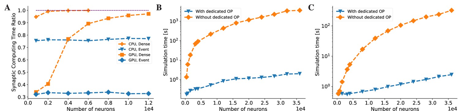
BrainPy accelerates the running speed of brain dynamics models through dedicated operators.
(A) Without dedicated event-driven operators, the majority of the time is spent on synaptic computations when simulating a COBA network model (Vogels and Abbott, 2005). The ratio significantly increases with the network size on both Central Processing Unit (CPU) and Graphics Processing Unit (GPU) devices (please refer to the lines labeled as ‘CPU, Dense’ and ‘GPU, Dense’ which correspond to the models utilizing the dense operator-based synaptic computation and running on the CPU and GPU devices, respectively). With the event-based primitive operators, the proportion of time spent on synaptic computation remains constant regardless of network size (please refer to the lines labeled as ‘CPU, Event’ and ‘GPU, Event’ which represent the models performing event-driven computations on the CPU and GPU devices, respectively). (B) On the CPU device, the COBA network model with event-based operators (see the ‘With dedicated OP’ line) is accelerated by up to three orders of magnitude compared to that without dedicated operators (see the ‘Without dedicated OP’ line). Please refer to Appendix 11—figure 7A for the acceleration ratio. (C) The COBA network model exhibited two orders of magnitude acceleration when implemented with event-based primitive operators on a GPU device. This performance improvement was more pronounced for larger network sizes on both CPU and GPU platforms. Please refer to Appendix 11—figure 7B for the acceleration ratio. For experimental details, please see Appendix 11.
Figure 8
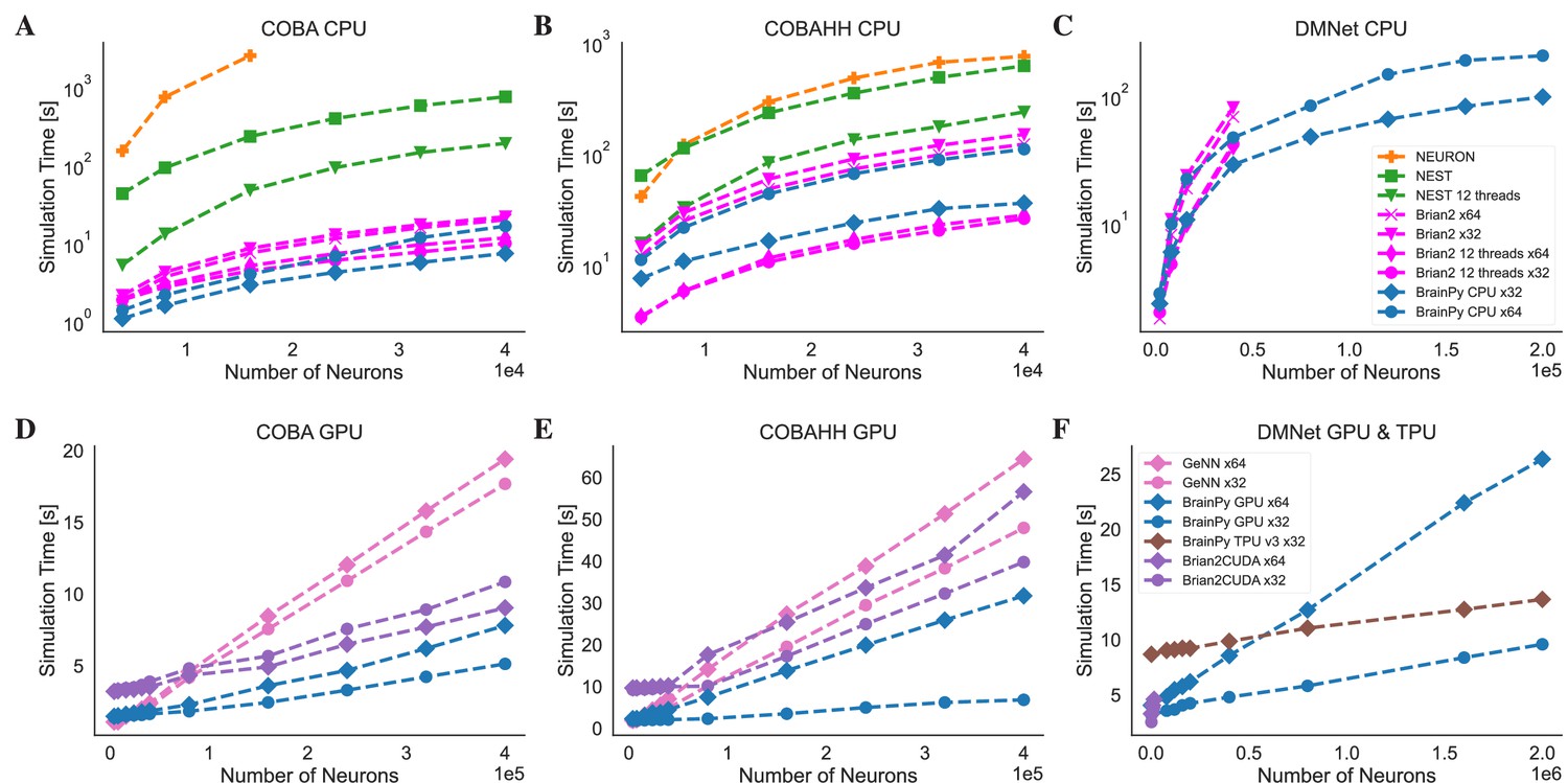
Speed comparison of NEURON, Nest, Brian2, and BrainPy under different computing devices.
Comparing speeds of different brain simulation platforms using the benchmark model COBA (Vogels and Abbott, 2005) on both the Central Processing Unit (CPU) (A) and Graphics Processing Unit (GPU) (D) devices. NEURON is truncated at 16,000 neurons due to its very slow runtime. Comparing speeds of different platforms using the benchmark model COBAHH (Brette et al., 2007) on both the CPU (B) and GPU (E) devices. Speed comparison of a spiking decision-making network (Wang, 2002) on CPU (C), GPU, and Tensor Processing Unit (TPU) (F) devices. Please refer to Appendix 11 for experimental details, and Appendix 11—figure 8 for more data.
Figure 9
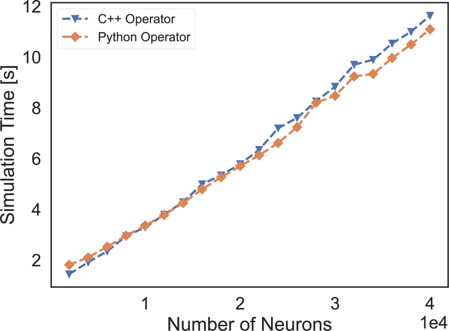
The speed comparison of event-based operators customized by C++ XLA custom call and our Python-level registration interface.
‘C++ Operator’ presents the simulation time of a COBA network using the event-based operator coded by C++, and ‘Python Operator’ shows the simulation speed of the network that is implemented through our operator registered by the Python interface.
Appendix 3—figure 1
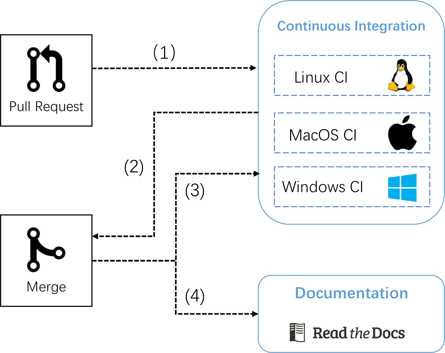
The pipeline of automatic continuous integration and documentation building in BrainPy.
Appendix 5—figure 1
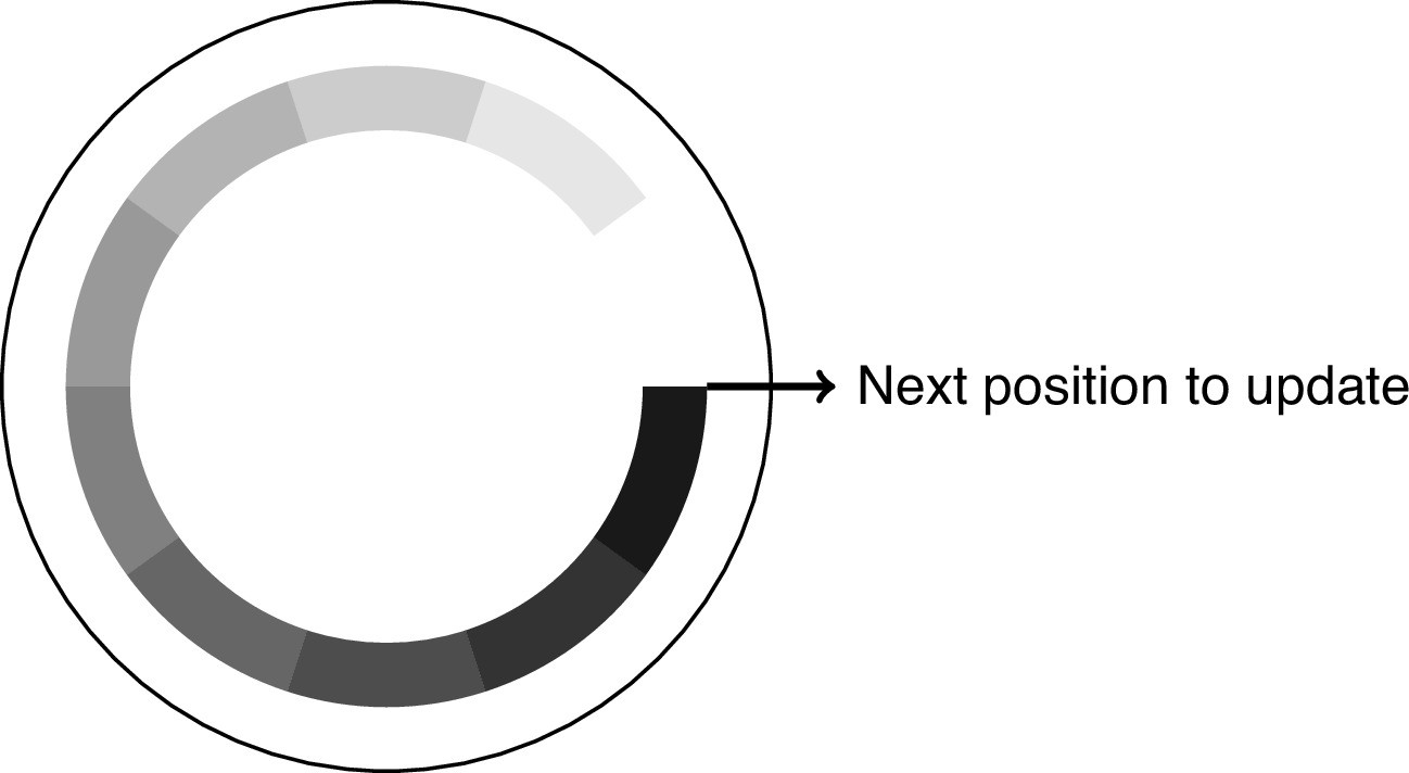
The dynamic array to store the delay buffer.
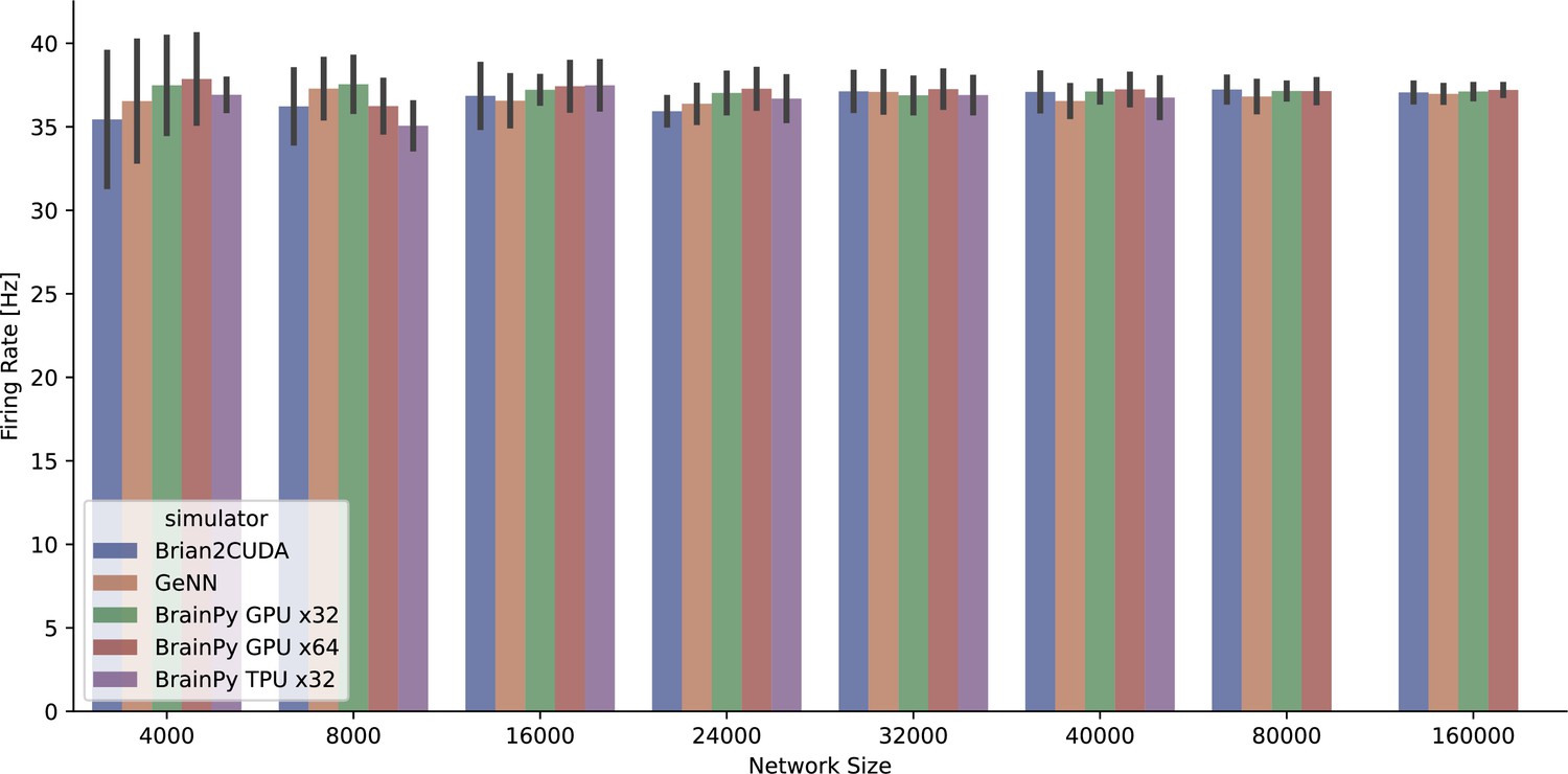
Appendix 11—figure 1
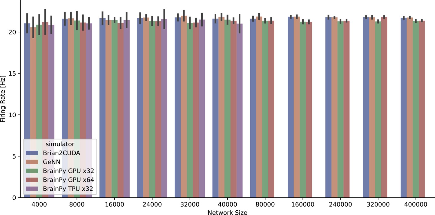
The average firing rate per neuron of the COBA network model (Vogels and Abbott, 2005) was measured across various simulators running on both GPU and TPU devices.
However, it should be noted that the BrainPy TPU x32 simulation was limited to 40,000 neurons due to memory constraints, resulting in a truncated network size.
Appendix 11—figure 2
The average firing rate per neuron of the COBAHH network model (Brette et al., 2007) was measured across various simulators running on both GPU and TPU devices.
However, it should be noted that the BrainPy TPU x32 simulation was limited to 40,000 neurons due to memory constraints, resulting in a truncated network size.
Appendix 11—figure 3
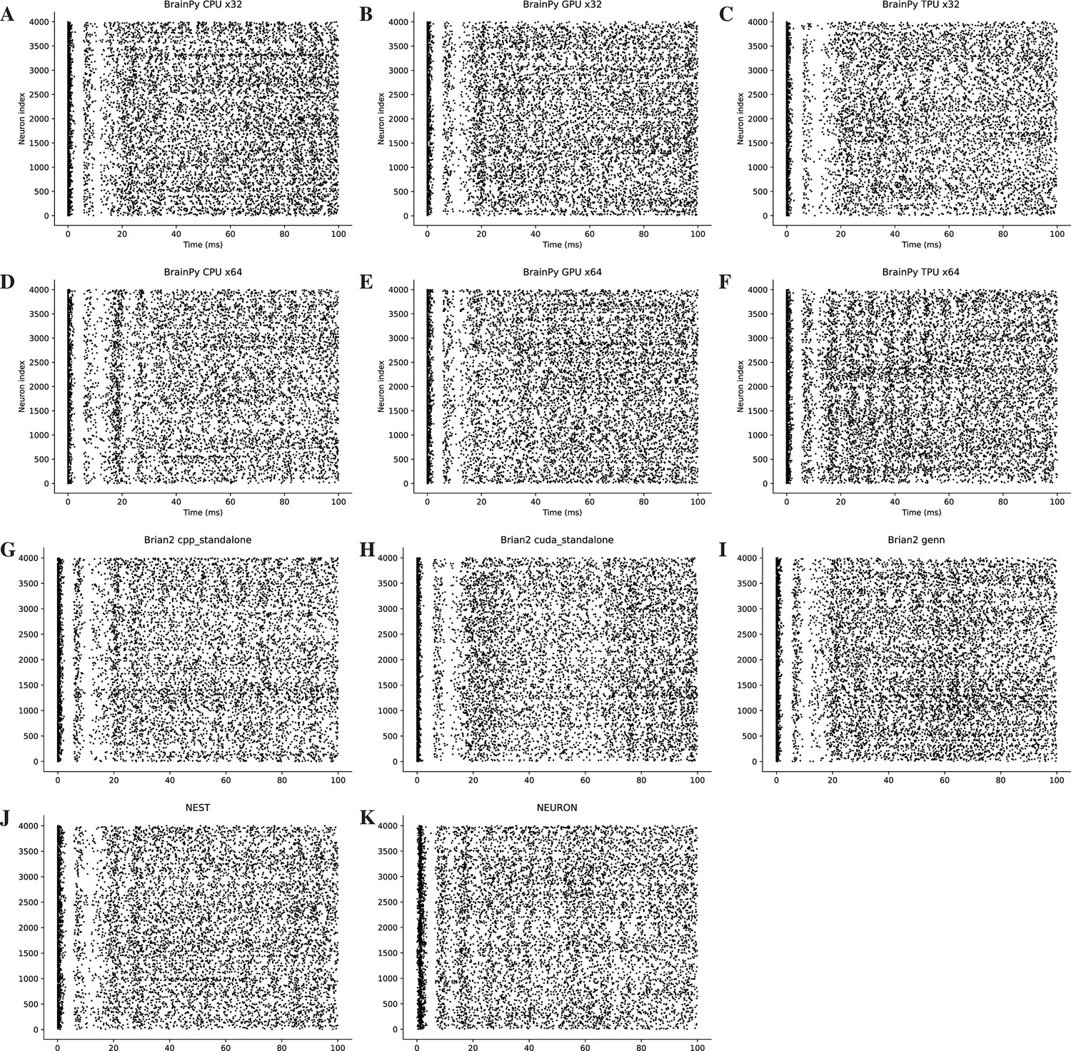
Rater diagrams of COBA network model with 4000 neurons (Vogels and Abbott, 2005) across different simulators on CPU, GPU, and TPU devices.
Here, we only present the simulation results for the initial 100 ms of the experiment.
Appendix 11—figure 4
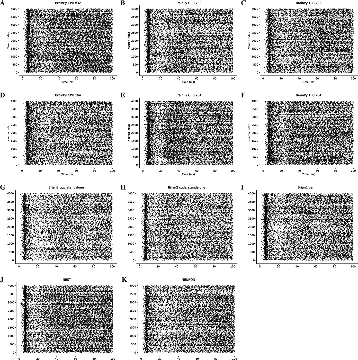
Rater diagrams of COBAHH network model with 4000 neurons (Brette et al., 2007) across different simulators on CPU, GPU, and TPU devices.
Here, we only present the simulation results for the initial 100 ms of the experiment.
Appendix 11—figure 5
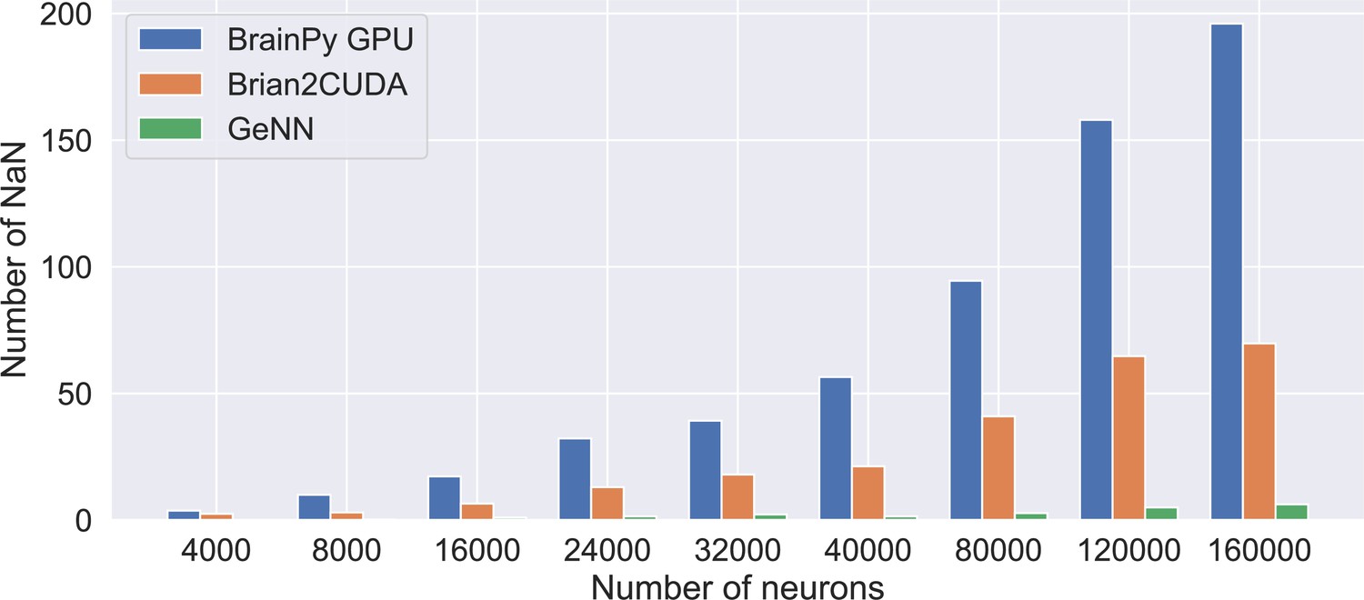
Number of neurons with NaN membrane potential after performing a 5-s long simulation of the COBAHH network model using the single-precision floating point.
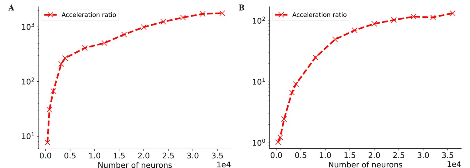
Appendix 11—figure 6
The acceleration ratio of JIT compilation on LIF neuron models (Abbott, 1999) and COBA network models (Vogels and Abbott, 2005).
(A) The acceleration ratio of just-in-time (JIT) compilation on the LIF neuron model is shown in the plot. The plotted values represent the simulation time ratios of the LIF neuron without JIT and with JIT. The top panel illustrates the acceleration on the CPU device, while the bottom panel demonstrates the acceleration on the GPU device. The acceleration ratios on both devices are approximately five times faster. (B) The simulation time ratio of the dense operator compared to the LIF neuron model with JIT compilation is shown. The top panel displays the time ratio on the CPU device, and the bottom panel demonstrates the time ratio on the GPU device. The simulation time ratios on both devices are nearly one, indicating that the jitted LIF neuron, with the same number of floating-point operations (FLOPs) as the ‘Dot’ operation, can run equivalently fast. (C) The acceleration ratio of the COBA network model (Vogels and Abbott, 2005) with JIT compilation compared to the model without JIT compilation on the CPU device is shown. The plot demonstrates a tenfold increase in speed after JIT compilation on the CPU device. (D) Similar to (C), the experiments were conducted on the GPU. Please refer to Figure 6 for the original data.
Appendix 11—figure 7
The acceleration ratio of dedicated operators of COBA network model (Vogels and Abbott, 2005) on both CPU (A) and GPU (B) devices.
Please refer to Figure 7 for the original data.
Appendix 11—figure 8
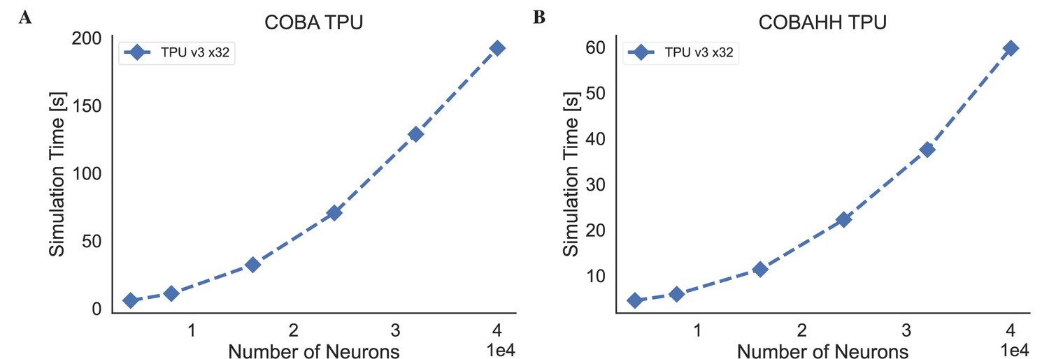
The simulation speeds of BrainPy on kaggle TPU v3-8 device.
(A) The simulation time of the COBA (Vogels and Abbott, 2005) network model across different network sizes. (B) The simulation time of the COBAHH (Brette et al., 2007) network model across different network sizes.
Tables
Appendix 4—table 1
Number of mathematical operators implemented in BrainPy.
This list will continue to expand since BrainPy will continue to add more operators for brain dynamics modeling. The list of implemented operators is online available at https://brainpy.readthedocs.io/en/latest/apis/math.html.
| Number | |
|---|---|
| Dense operators with NumPy syntax | 472 |
| Dense operators with TensorFlow syntax | 25 |
| Dense operators with PyTorch syntax | 10 |
| Sparse and event-driven operators | 20 |
Appendix 5—table 1
Numerical solvers provided in BrainPy for ordinary differential equations.
| Solver type | Solver name | Keyword |
|---|---|---|
| Runge–Kutta method | Euler | euler |
| Midpoint | midpoint | |
| Heun’s second-order method | heun2 | |
| Ralston’s second-order method | ralston2 | |
| Second-order Runge–Kutta method | rk2 | |
| Third-order Runge–Kutta method | rk3 | |
| Four-order Runge–Kutta method | rk4 | |
| Heun’s third-order method | heun3 | |
| Ralston’s third-order method | ralston3 | |
| Third-order strong stability preserving Runge–Kutta method | ssprk3 | |
| Ralston’s fourth-order method | ralston4 | |
| Fourth-order Runge–Kutta method with 3/8-rule | rk4_38rule | |
| Adaptive Runge–Kutta method | Runge–Kutta–Fehlberg 4 (5) | rkf45 |
| Runge–Kutta–Fehlberg 1 (2) | rkf12 | |
| Dormand–Prince method | rkdp | |
| Cash–Karp method | ck | |
| Bogacki–Shampine method | bs | |
| Heun–Euler method | heun_euler | |
| Exponential method | Exponential Euler method | exp_euler |
Appendix 5—table 2
Numerical solvers provided in BrainPy for stochastic differential equations.
‘Y’ denotes support. ‘N’ denotes not support.
| Integral type | Solver name | Keyword | Scalar Wiener | Vector Wiener |
|---|---|---|---|---|
| Itô integral | Strong SRK scheme: SRI1W1 | srk1w1_scalar | Y | N |
| Strong SRK scheme: SRI2W1 | srk2w1_scalar | Y | N | |
| Strong SRK scheme: KlPl | KlPl_scalar | Y | N | |
| Euler method | euler | Y | Y | |
| Milstein method | milstein | Y | Y | |
| Derivative-free Milstein method | milstein2 | Y | Y | |
| Exponential Euler | exp_euler | Y | Y | |
| Stratonovich integral | Euler method | euler | Y | Y |
| Heun method | heun | Y | Y | |
| Milstein method | milstein | Y | Y | |
| Derivative-free Milstein method | milstein2 | Y | Y |
Appendix 5—table 3
Numerical solvers provided in BrainPy for fractional differential equations.
| Derivative type | Solver name | Keyword |
|---|---|---|
| Caputo derivative | L1 schema | l1 |
| Euler method | euler | |
| Grünwald–Letnikov derivative | Short Memory Principle | short-memory |
Appendix 9—table 1
The weighted connectivity matrix among five brain areas: V1, V2, V4, TEO, and TEpd (Markov et al., 2014).
| V1 | V2 | V4 | TEO | TEpd | |
|---|---|---|---|---|---|
| V1 | 0.0 | 0.7322 | 0.1277 | 0.2703 | 0.003631 |
| V2 | 0.7636 | 0.0 | 0.1513 | 0.003274 | 0.001053 |
| V4 | 0.0131 | 0.3908 | 0.0 | 0.2378 | 0.07488 |
| TEO | 0.0 | 0.02462 | 0.2559 | 0.0 | 0.2313 |
| TEpd | 0.0 | 0.000175 | 0.0274 | 0.1376 | 0.0 |
Appendix 9—table 2
The delay matrix (ms) among five brain areas: V1, V2, V4, TEO, and TEpd (Markov et al., 2014).
| V1 | V2 | V4 | TEO | TEpd | |
|---|---|---|---|---|---|
| V1 | 0. | 2.6570 | 4.2285 | 4.2571 | 7.2857 |
| V2 | 2.6570 | 0. | 2.6857 | 3.4857 | 5.6571 |
| V4 | 4.2285 | 2.6857 | 0. | 2.8 | 4.7143 |
| TEO | 4.2571 | 3.4857 | 2.8 | 0. | 3.0571 |
| TEpd | 7.2857 | 5.6571 | 4.7143 | 3.0571 | 0. |
Additional files
Download links
A two-part list of links to download the article, or parts of the article, in various formats.
Downloads (link to download the article as PDF)
Open citations (links to open the citations from this article in various online reference manager services)
Cite this article (links to download the citations from this article in formats compatible with various reference manager tools)
BrainPy, a flexible, integrative, efficient, and extensible framework for general-purpose brain dynamics programming
eLife 12:e86365.
https://doi.org/10.7554/eLife.86365


