Neural criticality from effective latent variables
- Department of Physics, New York University, United States
- Department of Physics, Department of Biology, Initiative in Theory and Modeling of Living Systems, Emory University, United States
- Department of Neuroscience, University of Minnesota Medical School, United States
Figures
Figure 1
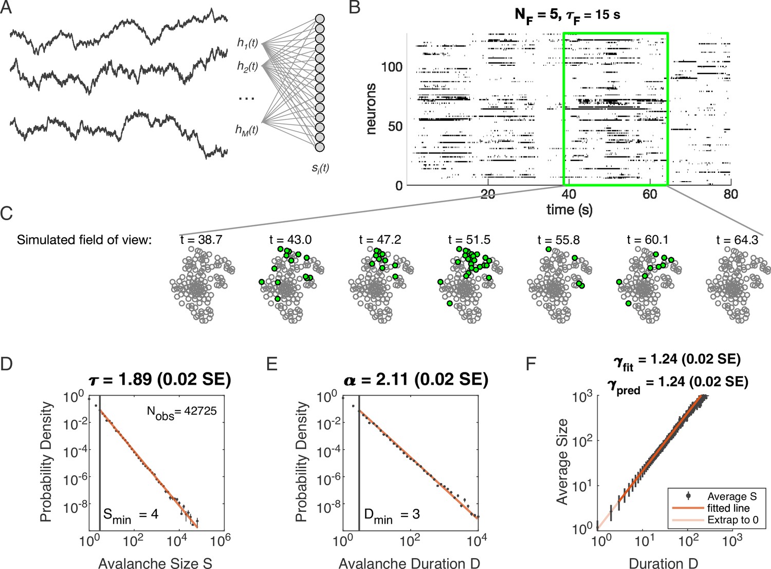
Latent dynamical variable model produces avalanche criticality.
Simulated network is neurons. Other parameters in Table 1. (A) Model structure. Latent dynamical variables are broadly coupled to neurons in the recorded population. (B) Raster plot of a sample of activity binned at 3 ms resolution across 128 neurons with five latent variables, each with correlation timescale . (C) Projection of activity into a simulated field of view for illustration. (D-F) Avalanche analysis in a network (parameters , , and ), showing size distribution (D), duration distribution (E), and size with duration scaling (F). Lower cutoffs used in fitting are shown with vertical lines and their values are indicated in the figures. There are avalanches of size in this simulated dataset. Estimated values of the critical exponents are shown in the titles of the panels.
Figure 2 with 4 supplements
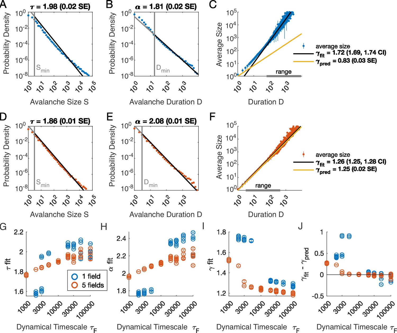
Multiple latent variables generate avalanche scaling at shorter timescales than a single latent variable.
Simulated network is neurons. Other parameters used for simulations for this figure are found in Table 2. (A-C) Scaling analysis for one variable models where the dynamic timescale is equal to 5×10³ time steps. (A) Distribution of avalanche sizes. MLE value of exponent for best-fit power law is (0.02 SE), with lower cutoff indicated by the vertical line. (B) Distribution of avalanche duration. MLE value of is 1.81 (0.02 SE). (C) Average size plotted against avalanche duration (blue points), with power-law fit (black line) and predicted relationship (yellow line) from MLE values for exponents in A and B. Gray bar on the horizontal axis indicates range, over which a power law with fits the data (see Materials and methods). (D-F) Analysis of avalanches from a simulation of a population coupled to five independent latent variables where the dynamic timescale is equal to 5×10³ time steps. (G) Exponents for avalanche size distributions across timescales for one-variable (blue) and five-variable (red) simulations. Each circle is a simulation with independently drawn coupling parameters. Simulations had to show scaling over at least two decades to be included in panels (G–J). (H) Exponents for avalanche duration distributions for simulations in G. (I) Fitted values of for simulations in G. (J) Difference between fitted and predicted values. Five-variable simulations produce crackling over a wider range of timescales than single-variable simulations.
Figure 2—figure supplement 1
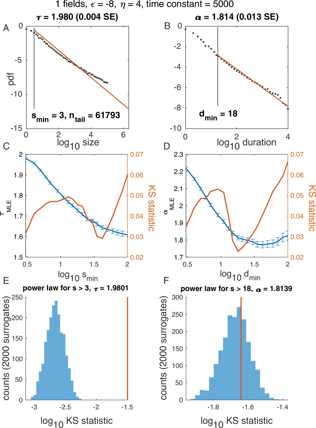
Illustration of algorithm for determining and , using one variable example in Figure 2.
(A-B) Probability density function for avalanche size (A) and duration (B) on a log-log scale, with the best power law fit (red). (C-D) In blue: Maximum likelihood exponent of a power-law model as a function of the minimum (lower cutoff) size (C) and duration (D). In red: KS statistics (see Materials and methods) for each fit. ‘Best fit‘ is the power law with the minimum KS statistic. (E-F) Surrogate data procedure. To generate each surrogate, samples were drawn from a power law with size / duration cutoff indicated (E, ; F, ) and the KS statistic was computed. Histograms illustrate KS statistic across surrogates (blue), while values derived from data are in red. Because the red line does not fall within the blue histogram, the hypothesis that the data is fitted well by a power law fit was rejected in E. At the same time, since the red line falls within the blue histogram in F, the hypothesis was accepted.
Figure 2—figure supplement 2
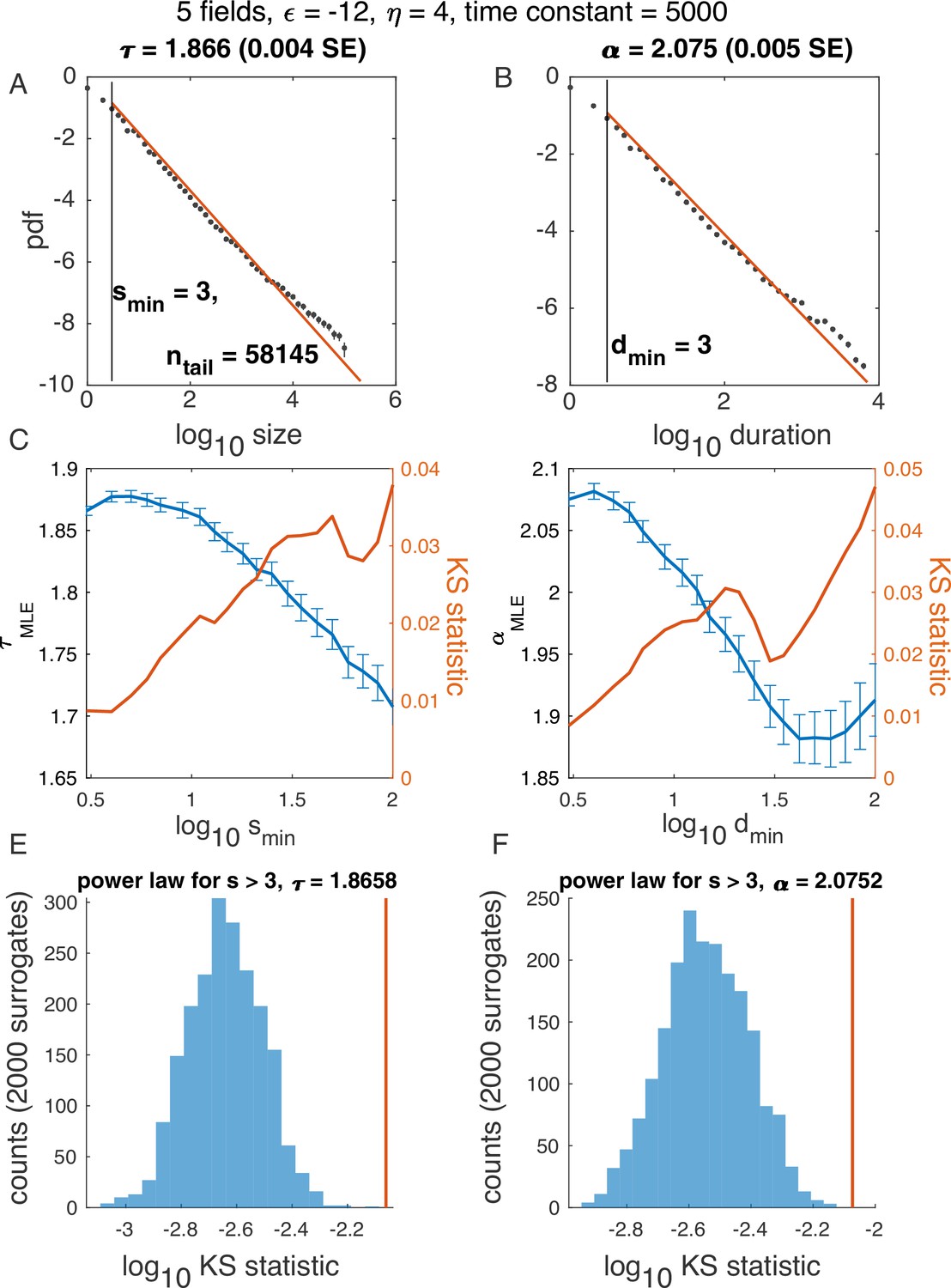
Illustration of algorithm for determining and , using example in Figure 2, five latent variables.
Notation the same as in Figure 2—figure supplement 3.
Figure 2—figure supplement 3
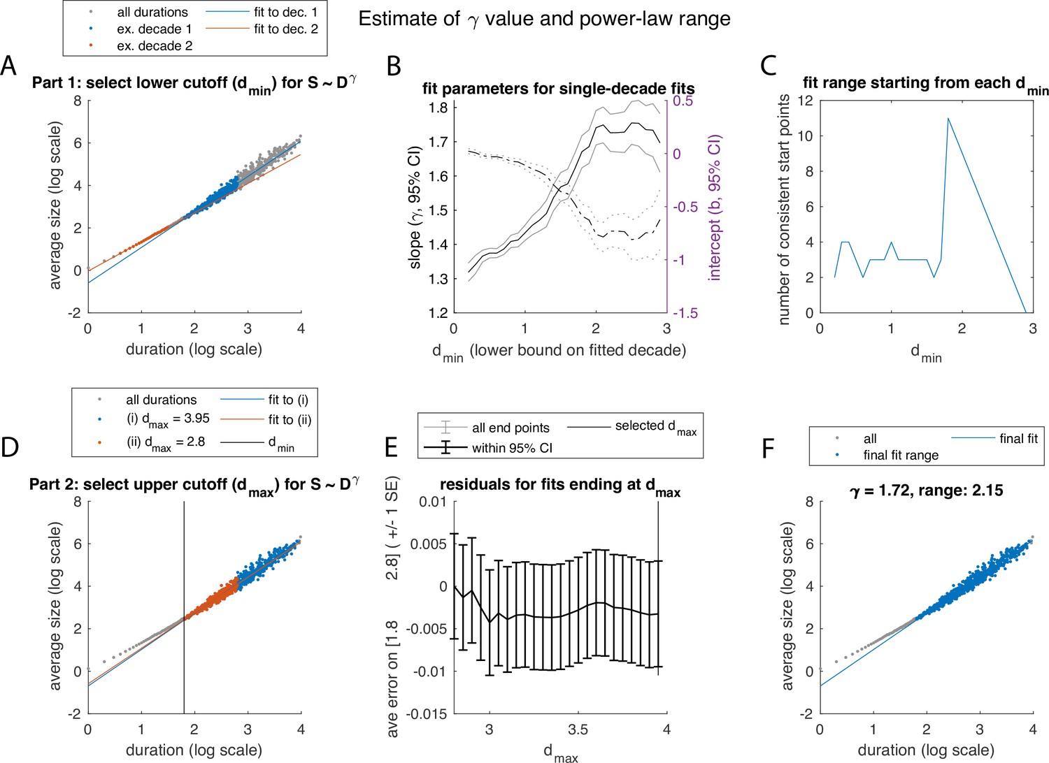
Illustration of algorithm for fitting the exponent and determining the range, over which power law scaling of average size with duration is observed, using example in Figure 2(A–D).
(A-C) Determining the lower bound, the minimum duration . (A) The relation was fit using linear least-squares, restricted to (overlapping) 1-decade ranges (blue, red: example decades). (B) Confidence intervals for fit parameters () for fits starting at each value of . (C) Best value of was selected based on how many subsequent start points yielded consistent slope/intercept values. (D-F) Determining the upper bound, maximum duration. (D) Keeping fixed based of value obtained in C, we test values of up to the maximum duration event, and fit over the range. (E) Average residual over the fit range , calculated for each fit and plotted against the value of used for that fit. The largest value of without evidence of bias in the residual was then selected. (F) Final fit and range.
Figure 2—figure supplement 4
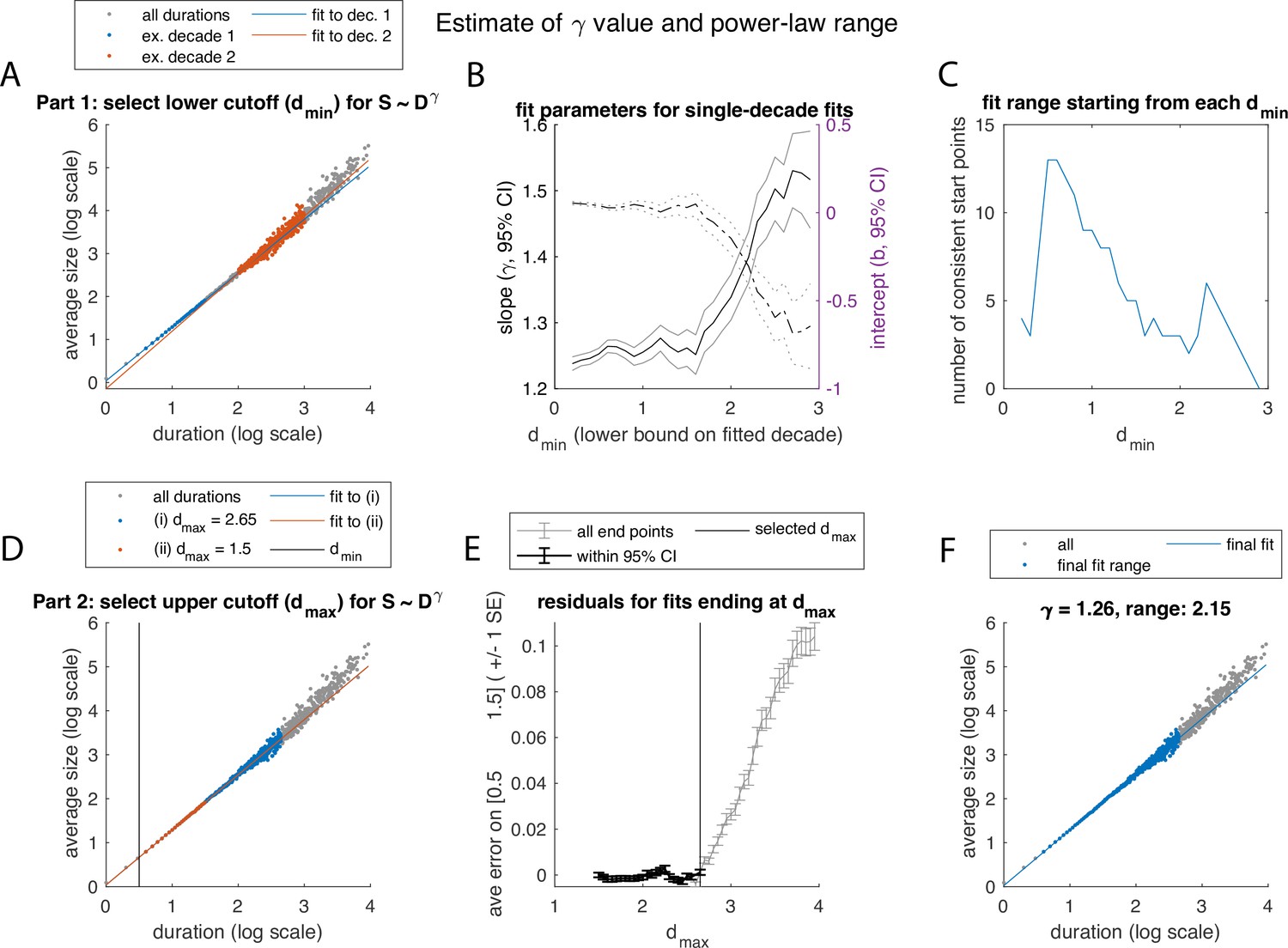
Illustration of algorithm for fitting the exponent and determining the range over which power-law scaling of average size with duration is observed, using example in Figure 2E–H.
See Figure 2—figure supplement 2 for caption. In this example, a lower value of was selected. Panel E, which was flat for Figure 2—figure supplement 2, now shows how extending the range to high values of can generate systematic errors at the low range of the fit, even while having a high overall goodness of fit metric.
Figure 3
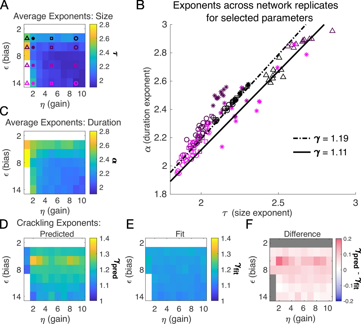
Exponents across network simulations for networks of neurons.
Each parameter combination was simulated for ten replicates, each time drawing randomly the couplings , the latent variable values, and the neural activities. Other parameters in Table 3. (A) Average across replicates for the size exponent . (B) Scatter plot of vs. for each network replicate for parameter combinations indicated in A. Linear relationships between and , corresponding to the minimum and maximum values of from panel E, are shown to guide the eye. (C) Same as A, for duration exponent . (D) Predicted exponent, , derived from A and C. (E) Value of from fit to . (F) Difference between and .
Figure 4 with 1 supplement
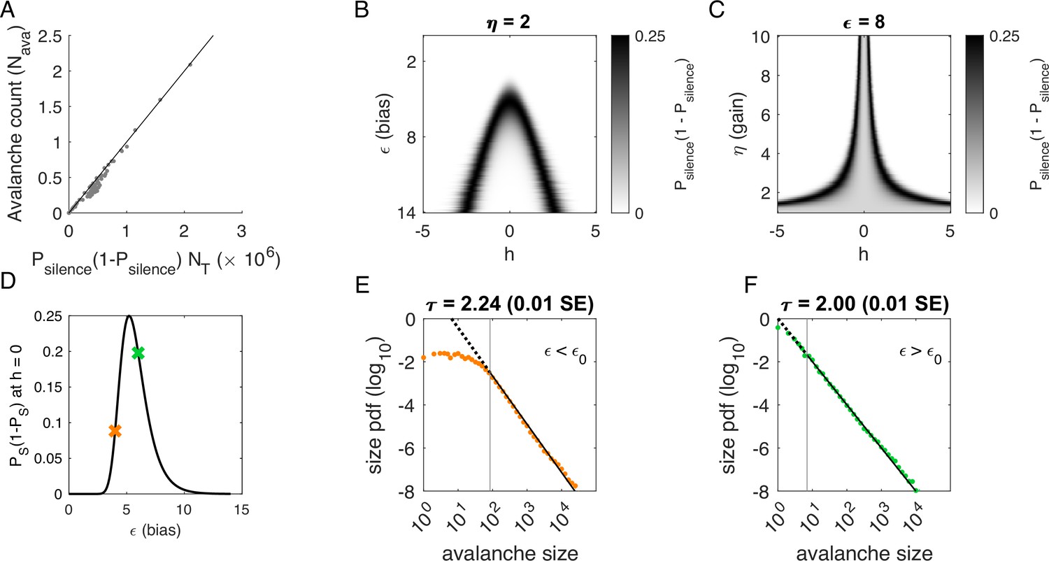
Avalanches in the latent dynamical variable model with a single quasistatic variable.
Parameters in Table 3. (A) Number of avalanches in simulations from Figure 3 as a function of the calculated probability of avalanches at fixed across values of and latent variable . Line indicates equality. (B) Probability of avalanches with across values of and . The latent variable is normally distributed with mean 0 and variance 1. Where the distribution of overlaps with regions of high probability (black), avalanches occur. (C) Probability of avalanches at across values of and . Increasing narrows the range of that generates avalanches. (D) Probability of avalanches at for a populations of 128 neurons (black line) and for a varying . Size distributions corresponding to simulations marked by the green and orange crosses are in E, F. (E) Example of size distribution with (orange marker in D). Size cutoff is close to 100. (F) Example of size distribution with (green marker in D). Size cutoff is < 10.
Figure 4—figure supplement 1

Estimate of how long it takes to observe avalanche criticality at each combination of and .
We took a parameter combination with a low rate of avalanches but good apparent scaling ( and ) and assumed that this is a reasonable estimate of the minimum number of observations (approximately 106 avalanches) required to observe scaling. To translate to observation length (in hours), we divided the number of avalanches observed in each full-length simulation by this minimum count and converted to a time using a time bin of 10ms. Simulations were for a recorded population of 128 neurons. For this size of population, .
Figure 5
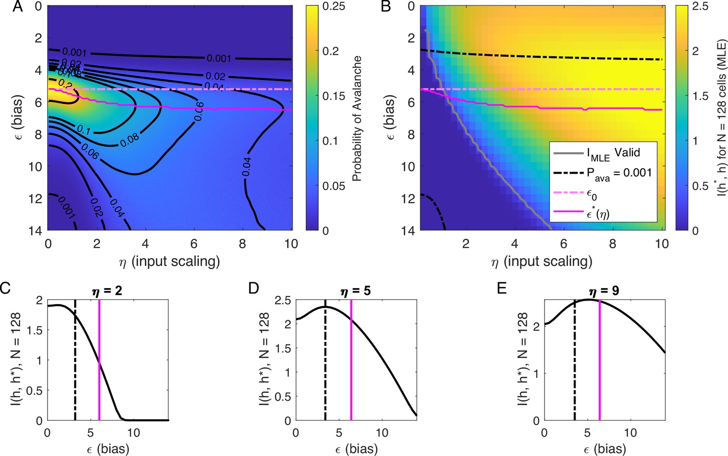
Information in the neural activity about the latent variable is higher in the low- avalanche region, compared to high- avalanche or high-rate avalanche-free activity.
(A) Probability of avalanche per time step across values of and . Solid magenta curve follows , the value of maximizing the probability of avalanches at fixed . Dashed magenta line indicates , calculated analytically, which matches at . (B) Information about latent variable, calculated from maximum likelihood estimate of using population activity. MLE approximation is invalid in the dark-blue region bounded by gray curve. Magenta line marks the maximum values of , reproduced from A. Dashed black curve indicates . The highest information region falls between and the contour for . (C - E) Slices of B, showing for . Magenta and dashed black lines again indicate and , respectively, as in B. Black dashed line marks the approximate boundary between the high-activity/no avalanche and the high-cutoff avalanche, and magenta line marks boundary between high-cutoff and low-cutoff avalanche regions.
Tables
Table 1
Simulation parameters for Figure 1.
| Parameter | Description | Value |
|---|---|---|
| bias towards silence | ||
| variance multiplier | ||
| number of latent fields | ||
| latent field time constant | ||
| number of cells |
Table 2
Simulation parameters for Figure 2.
| Parameter | Description | Value |
|---|---|---|
| bias towards silence | (for ) or (for ) | |
| variance multiplier | ||
| number of latent fields | ||
| latent field time constant | ||
| number of cells |
Additional files
-
MDAR checklist
- https://cdn.elifesciences.org/articles/89337/elife-89337-mdarchecklist1-v1.pdf
-
Source code 1
Code (Python and MATLAB) used to run simulations, analyses, and calculations.
- https://cdn.elifesciences.org/articles/89337/elife-89337-code1-v1.zip
Download links
A two-part list of links to download the article, or parts of the article, in various formats.
Downloads (link to download the article as PDF)
Open citations (links to open the citations from this article in various online reference manager services)
Cite this article (links to download the citations from this article in formats compatible with various reference manager tools)
Neural criticality from effective latent variables
eLife 12:RP89337.
https://doi.org/10.7554/eLife.89337.3


