Research Article

Efficient estimation for large-scale linkage disequilibrium patterns of the human genome

Institute of Bioinformatics, Zhejiang University, China
Center for General Practice Medicine, Department of General Practice Medicine, Zhejiang Provincial People’s Hospital, People’s Hospital of Hangzhou Medical College, China
Center for Reproductive Medicine, Department of Genetic and Genomic Medicine, and Clinical Research Institute, Zhejiang Provincial People’s Hospital, People’s Hospital of Hangzhou Medical College, China
Hainan Institute of Zhejiang University, China
Alibaba Group, China
Key Laboratory of Endocrine Gland Diseases of Zhejiang Province, China

Dec 27, 2023

https://doi.org/10.7554/eLife.90636.3

Open access
Copyright information

Figures
Tables
Additional files

7 figures, 5 tables and 2 additional files

Figures

Figure 1

Download asset Open asset

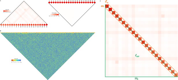
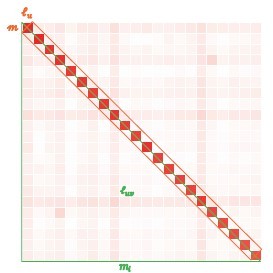
Schematic illustration for large-scale linkage disequilibrium (LD) analysis as exampled for CONVERGE cohort.

(A) The 22 human autosomes have consequently 22 ${\hat{l}}_{i}$ and 231 ${\hat{l}}_{i \cdot j}$ , without (left) and with (right) scaling transformation; Scaling transformation is given in Equation 8. (B) If zoom into chromosome 2 of 420,946 single-nucleotide polymorphisms (SNPs), a chromosome of relative neutrality is expected to have self-similarity structure that harbors many approximately strong ${\hat{l}}_{u}$ along the diagonal, and relatively weak ${\hat{l}}_{u v}$ off-diagonally. Here chromosome 2 of CONVERGE has been split into 1000 blocks and yielded 1000 ${\hat{l}}_{u}$ LD grids, and 499,500 ${\hat{l}}_{u v}$ LD grids. (C) An illustration of the construction process for the LD-decay regression model.

Figure 2 with 2 supplements

Download asset Open asset

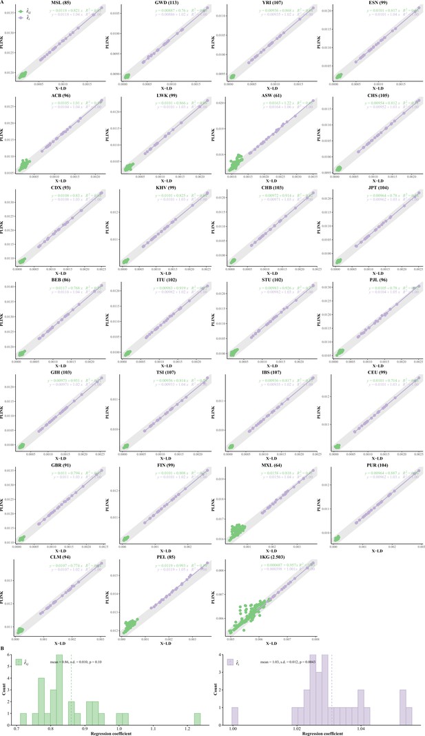
Reconciliation for linkage disequilibrium (LD) estimators in the 26 cohorts of 1KG.

(A) Consistency examination for the 26 1KG cohorts for their ${\hat{l}}_{i}$ and ${\hat{l}}_{i \cdot j}$ estimated by X-LD and PLINK (--r2). In each figure, the 22 ${\hat{l}}_{i}$ fitting line is in purple, whereas the 231 ${\hat{l}}_{i \cdot j}$ fitting line is in green. The gray solid line, $y = \frac{1}{n} + x$ , in which $n$ the sample size of each cohort, represents the expected fit between PLINK and X-LD estimates, and the two estimated regression models at the top-right corner of each plot show this consistency. The sample size of each cohort is in parentheses. (B) Distribution of $R^{2}$ of ${\hat{l}}_{i}$ and ${\hat{l}}_{i \cdot j}$ fitting lines is based on X-LD and PLINK algorithms in the 26 cohorts; $R^{2}$ represents variation explained by the fitted model. 26 1KG cohorts: MSL (Mende in Sierra Leone), GWD (Gambian in Western Division, The Gambia), YRI (Yoruba in Ibadan, Nigeria), ESN (Esan in Nigeria), ACB (African Caribbean in Barbados), LWK (Luhya in Webuye, Kenya), ASW (African Ancestry in Southwest US), CHS (Han Chinese South), CDX (Chinese Dai in Xishuangbanna, China), KHV (Kinh in Ho Chi Minh City, Vietnam), CHB (Han Chinese in Beijing, China), JPT (Japanese in Tokyo, Japan), BEB (Bengali in Bangladesh), ITU (Indian Telugu in the UK), STU (Sri Lankan Tamil in the UK), PJL (Punjabi in Lahore, Pakistan), GIH (Gujarati Indian in Houston, TX), TSI (Toscani in Italia), IBS (Iberian populations in Spain), CEU (Utah residents [CEPH] with Northern and Western European ancestry), GBR (British in England and Scotland), FIN (Finnish in Finland); MXL (Mexican Ancestry in Los Angeles, CA), PUR (Puerto Rican in Puerto Rico), CLM (Colombian in Medellin, Colombia), and PEL (Peruvian in Lima, Peru).

Figure 2—figure supplement 1

Download asset Open asset

Reconciliation for linkage disequilibrium (LD) estimators in AFR, EAS, and EUR.

In each figure, the 22 ${\hat{l}}_{i}$ fit line is in purple, whereas the 231 ${\hat{l}}_{i \cdot j}$ fit line is in green. The gray solid line, $y = \frac{1}{n} + x$ , in which $n$ the sample size, represents the expected fit between PLINK and X-LD, and the two estimated regression models at the top-right corner show this consistency.

Figure 2—figure supplement 2

Download asset Open asset

The computational efficiency of X-LD algorithm.

Considering the high computational cost of PLINK, only the first chromosome was chosen. In the process of evaluating computational efficiency, we kept adding single-nucleotide polymorphisms (SNPs) until the inclusion of the entire chromosome. The bar chart and line chart show the actual calculation time and theoretical calculation complexity, respectively.

Figure 3 with 1 supplement

Download asset Open asset

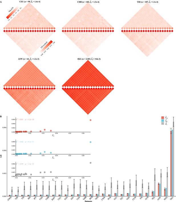
Various linkage disequilibrium (LD) components for the 26 1KG cohorts.

(A) Chromosomal scale LD components for five representative cohorts (CEU, CHB, YRI, ASW, and 1KG). The upper parts of each figure represent ${\hat{l}}_{i}$ (along the diagonal) and ${\hat{l}}_{i \cdot j}$ (off-diagonal), and the lower part ${\hat{\tilde{l}}}_{i \cdot j}$ as in Equation 8. For visualization purposes, the quantity of LD before scaling is transformed to a -log10 scale, with smaller values (red hues) representing larger LD, and a value of 0 representing that all single-nucleotide polymorphisms (SNPs) are in LD. (B) The relationship between the degree of population structure (approximated by ${\bar{F}}_{s t}$ ) and ${\hat{l}}_{i}$ , ${\hat{l}}_{g}$ , and ${\hat{l}}_{i \cdot j}$ in the 26 1KG cohorts.

Figure 3—figure supplement 1

Download asset Open asset

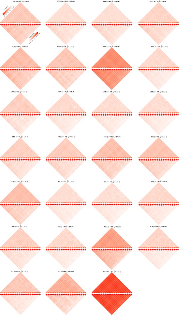
Chromosomal scale linkage disequilibrium (LD) components for 26 cohorts in 1KG.

The upper and lower parts of each figure represent the LD before and after scaling according to Equation 8. ${\hat{l}}_{i}$ and ${\hat{l}}_{i \cdot j}$ are represented by the diagonal and the off-diagonal elements, respectively. For visualization purposes, LD before scaling is transformed to a -log10-scale, with smaller values (red hues) representing larger LD, and a value of 0 representing that all single-nucleotide polymorphisms (SNPs) are in LD.

Figure 4 with 2 supplements

Download asset Open asset

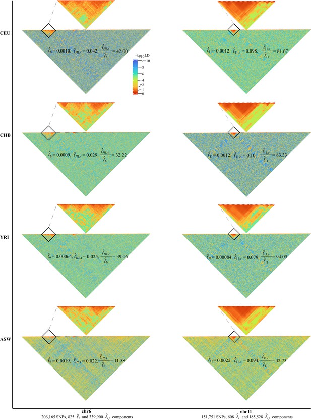
High-resolution illustration for linkage disequilibrium (LD) grids for CEU, CHB, YRI, and ASW ( $m = 250$ ).

For each cohort, we partition chromosomes 6 and 11 into high-resolution LD grids (each LD grid contains 250 ×250 single-nucleotide polymorphism [SNP] pairs). The bottom half of each figure shows the LD grids for the entire chromosome. Further zooming into HLA on chromosome 6 and the centromere region on chromosome 11, and their detailed LD in the relevant regions are also provided in the upper half of each figure. For visualization purposes, LD is transformed to a -log10-scale, with smaller values (red hues) representing larger LD, and a value of 0 representing that all SNPs are in LD.

Figure 4—figure supplement 1

Download asset Open asset

High-resolution illustration for linkage disequilibrium (LD) grids for CEU, CHB, YRI, and ASW ( $m = 500$ ).

For each cohort, we partitioned each chromosome into consecutive LD grids (each LD grid containing 500 single-nucleotide polymorphisms [SNPs]). For visualization purposes, LD is transformed to a -log10-scale, with smaller values (red hues) representing larger LD, and a value of 0 representing that all SNPs are in LD.

Figure 4—figure supplement 2

Download asset Open asset

Influence of HLA region on chromosome 6 and centromere region on chromosome 11 on chromosomal linkage disequilibrium (LD) in CEU, CHB, YRI, and ASW.

When another region was removed, to avoid chance, the same number of consecutive single-nucleotide polymorphisms (SNPs) as HLA region or centromere region was randomly removed from the genomic region, and this operation was repeated 100 times.

Figure 5 with 1 supplement

Download asset Open asset

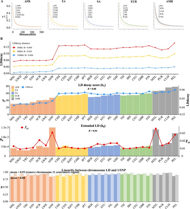
Linkage disequilibrium (LD) decay analysis for 26 1KG cohorts.

(A) Conventional LD decay analysis in PLINK for 26 cohorts. To eliminate the influence of sample size, the inverse of sample size has been subtracted from the original LD values. The YRI cohort, represented by the orange dotted line, is chosen as the reference cohort in each plot. The top-down arrow shows the order of LDdecay values according to Table 5. (B) Model-based LD decay analysis for the 26 1KG cohorts. We regressed each autosomal ${\hat{l}}_{i}$ against its corresponding inversion of the single-nucleotide polymorphism (SNP) number for each cohort. Regression coefficient $b_{1}$ quantifies the averaged LD decay of the genome and intercept $b_{0}$ provides a direct estimate of the possible existence of long-distance LD. The $R$ values in the first three plots indicate the correlation between ${\hat{b}}_{1}$ and LD decay score in three different physical distance and the correlation between ${\hat{b}}_{1}$ (left-side vertical axis) and LD decay score (right-side vertical axis) and the correlation between ${\hat{b}}_{0}$ (left-side vertical axis) and ${\bar{F}}_{s t}$ (right-side vertical axis), respectively. The last plot assessed the impact of centromere region of chromosome 11 on the linear relationship between chromosomal LD and the inverse of the SNP number. The dark and light gray dashed lines represent the mean of the $R$ with and without the presence of centromere region of chromosome 11.

Figure 5—figure supplement 1

Download asset Open asset

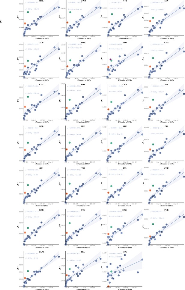
The correlation between the inverse of the single-nucleotide polymorphism (SNP) number and chromosomal linkage disequilibrium (LD) in 26 cohorts of 1KG.

Figure 6 with 1 supplement

Download asset Open asset

The correlation between the inversion of the single-nucleotide polymorphism (SNP) number and ${\hat{l}}_{i}$ .

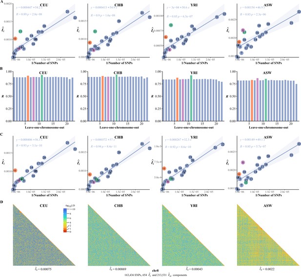
(A) The correlation between the inversion of the SNP number and ${\hat{l}}_{i}$ in CEU, CHB, YRI, and ASW. (B) Leave-one-chromosome-out strategy is adopted to evaluate the contribution of a certain chromosome on the correlation between the inverse of the SNP number and ${\hat{l}}_{i}$ . (C) The correlation between the inversion of the SNP number and chromosomal linkage disequilibrium (LD) in CEU, CHB, YRI, and ASW after removing the centromere region of chromosome 11. (D) High-resolution illustration for LD grids for chromosome 8 in CEU, CHB, YRI, and ASW. For each cohort, we partition chromosome 8 into consecutive LD grids (each LD grid contains 250 ×250 SNP pairs). For visualization purposes, LD is transformed to a -log10-scale, with smaller values (red hues) representing larger LD, and a value of 0 representing that all SNPs are in LD.

Figure 6—figure supplement 1

Download asset Open asset

Influence of expanding of single-nucleotide polymorphism (SNP) numbers on the correlation between the inverse of the SNP number and chromosomal linkage disequilibrium (LD) in ASW.

Randomly selected SNPs that were presented in ASW but were not 2,997,635 consensus SNPs were added to the ASW cohort to demonstrate the stable pattern of chromosome 8.

Author response image 1

Download asset Open asset

Tables

Table 1

Notation definitions.

Notation	Definition
$C$	The number of chromosomes.
$i$ and $j$	Subscripts index chromosome $i$ and $j$ .
$β_{i}$	The number of SNP segments of chromosome $i$ , each of which has $m$ SNPs.
$D_{l_{1} l_{2}}$	The difference between the observed and expected haplotype frequencies, with $D_{l_{1} l_{2}} = p_{l_{1} l_{2}} - p_{l_{1}} p_{l_{2}}$ .
$F$	The inbreeding coefficient.
$K_{i}$	Genetic relatedness matrix for chromosome $i$ , and two vectors, $k_{i_{o}}$ and $k_{i_{d}}$ , from $K_{i}$ , where $k_{i_{o}}$ stacks the off-diagonal elements and $k_{i_{d}}$ stacks the diagonal elements.
$k$	Subscript indexes individual.
$l_{1}$ and $l_{2}$	Subscripts index a pair of SNPs.
$m$	The number of SNPs; $m_{i}$ the number of SNPs on chromosome $i$ .
$n$	The number of samples; $n_{i}$ , the number of samples in subpopulation $i$ .
$p_{l}$ and $q_{l}$	Frequency of the lth reference allele and alternative allele in the population.
$θ_{k_{1} k_{2}}$	The relatedness score between individual $k_{1}$ and $k_{2}$ .
$x_{k l}$	The genotype for the kth individual at the lth biallelic locus.
$X_{i}$ and ${\tilde{X}}_{i}$	Genotype and standardized genotype matrixes for chromosome $i$ .
$ρ_{l_{1} l_{2}}^{2}$	Squared Pearson’s correlation coefficient for any pair of SNPs, including an SNP to itself when $l_{1} = l_{2}$ .
$r^{2}$	Squared Pearson’s correlation metric for LD but estimated from PLINK (--r2) or PopLDdecay.
$l_{g}$	The mean LD of the whole genome-wide $m^{2}$ SNP pairs.
$l_{i}$	The intra-chromosomal mean LD for the ith chromosome of $m_{i}^{2}$ SNP pairs.
$l_{i \cdot j}$	The inter-chromosomal mean LD ith and jth chromosomal $m_{i} m_{j}$ SNP pairs, a scaled version is ${\tilde{ℓ}}_{i j}$ .
$l_{u}$	The mean LD for a diagonal grid.
$l_{u v}$	The mean LD for off-diagonal grids.

LD, linkage disequilibrium; SNP, single-nucleotide polymorphism.

Table 2

Computational time for the demonstrated estimation tasks.

Cohort	Task description	Time cost	Computational time complex
CHB ( $n = 103$ , $m = 2,997,655$ )	Estimation for 22 autosomal $ℓ_{i}$ , and 231 inter-chromosomal $ℓ_{i \cdot j}$ . For results, see Figure 3 and Table 3.	101,34 s	$O (n^{2} m)$
1KG ( $n = 2,503$ , $m = 2,997,655$ )	Same as above.	3008.29 s	Same as above
CONVERGE ( $n = 10,640$ , $m = 5,215,820$ )	Same as above. For results, see Figure 1A.	77,508.00 s	Same as above
	Estimation for high-resolution LD interaction given bin size of 250 SNPs
CHB ( $n = 103$ , $m_{2} = 241,241$ )	Chromosome 2, estimation for 965 $l_{i}$ , and 465,130 $l_{i \cdot j}$ . For results, see Figure 4.	66.86 s	$O (n^{2} (m_{i} + {(\frac{m_{i}}{250})}^{2}))$
CHB ( $n = 103$ , $m_{22} = 40,378$ )	Chromosome 22, estimation for 162 $l_{i}$ , and 13,041 $l_{i \cdot j}$ . For results, see Figure 4.	3.22 s	Same as above
CONVERGE ( $n = 10,640$ , $m_{22} = 71,407$ )	Chromosome 22, estimation for 286 $l_{i}$ , and 40,755 $l_{i \cdot j}$ .	8,736.29 s	Same as above
CONVERGE ( $n = 10,640$ , $m_{2} = 420,949$ )	Chromosome 2, estimation for 1000 $l_{i}$ , and 499,500 $l_{i \cdot j}$ . For results, see Figure 1B.	45,125.00 s	Chromosome 2 was split into 1000 blocks, each of which had about 420 SNPs

For the sake of fair comparison, 10 CPUs were used for multi-thread computing.
LD, linkage disequilibrium; SNP, single-nucleotide polymorphism.

Table 3

X-LD estimation for complex LD components (2,997,635 SNPs).

Cohort ( $n$ )	Ancestry	$λ_{1} (F_{s t})$ *	${\hat{l}}_{g}$ (SE)^†	$\hat{{\bar{l}}_{i}}$ (SD) ^‡	$\hat{{\bar{l}}_{i \cdot j}}$ (SD) ^‡	${\hat{\tilde{l}}}_{i \cdot j}$ (SD) ^‡	Lower bound of LD ^§
MSL (85)	AFR	1.10 (0.013)	1.9e-4 (1.21e-6)	6.9e-4 (2.0e-4)	1.7e-4 (1.7e-5)	0.26 (0.053)	0.161971831
GWD (113)	AFR	1.07 (0.009)	1.1e-4 (5.61e-7)	6.0e-4 (2.0e-4)	8.7e-5 (8.1e-6)	0.16 (0.037)	0.247218789
YRI (107)	AFR	1.05 (0.010)	1.1e-4 (4.23e-7)	5.9e-4 (2.0e-4)	8.8e-5 (6.9e-6)	0.16 (0.04)	0.242001641
ESN (99)	AFR	1.09 (0.011)	1.4e-4 (7.67e-7)	7.0e-4 (2.2e-4)	1.2e-4 (1.2e-5)	0.19 (0.043)	0.217391304
ACB (96)	AFR	2.01 (0.021)	2.9e-4 (3.78e-6)	9.1e-4 (2.5e-4)	2.5e-4 (3.6e-5)	0.29 (0.070)	0.147727273
LWK (99)	AFR	1.35 (0.014)	2.2e-4 (2.38e-6)	8.4e-4 (2.5e-4)	1.9e-4 (3.2e-5)	0.24 (0.052)	0.173913043
ASW (61)	AFR	1.90 (0.031)	1.1e-3 (2.73e-5)	2.0e-3 (3.2e-4)	1.1e-3 (6.2e-5)	0.57 (0.059)	0.079681275
CHS (105)	EA	1.08 (0.010)	1.4e-4 (9.39e-7)	9.5e-4 (3.4e-4)	1.0e-4 (1.3e-5)	0.12 (0.030)	0.31147541
CDX (93)	EA	1.11 (0.012)	1.8e-4 (1.38e-6)	1.1e-3 (3.6e-4)	1.4e-4 (2.0e-5)	0.14 (0.040)	0.272277228
KHV (99)	EA	1.07 (0.011)	1.4e-4 (7.67e-7)	9.5e-4 (3.5e-4)	1.0e-4 (1.2e-5)	0.12 (0.031)	0.31147541
CHB (103)	EA	1.07 (0.010)	1.3e-4 (6.94e-7)	9.3e-4 (3.4e-4)	9.5e-5 (1.1e-5)	0.11 (0.030)	0.317948718
JPT (104)	EA	1.06 (0.010)	1.3e-4 (7.22e-7)	1.0e-3 (3.8e-4)	9.3e-5 (1.2e-5)	0.10 (0.028)	0.338638673
BEB (86)	SA	1.07 (0.012)	1.7e-4 (8.09e-7)	9.1e-4 (3.1e-4)	1.4e-4 (1.5e-5)	0.17 (0.042)	0.236363636
ITU (102)	SA	1.61 (0.016)	1.9e-4 (1.84e-6)	9.5e-4 (3.1e-4)	1.5e-4 (1.7e-5)	0.18 (0.044)	0.231707317
STU (102)	SA	1.56 (0.015)	2.6e-4 (3.21e-6)	1.0e-3 (3.3e-4)	2.3e-4 (3.1e-5)	0.23 (0.047)	0.171526587
PJL (96)	SA	1.67 (0.017)	2.4e-4 (2.74e-6)	1.1e-3 (3.4e-4)	2.0e-4 (2.2e-5)	0.21 (0.048)	0.20754717
GIH (103)	SA	1.73 (0.017)	2.7e-4 (3.41e-6)	1.1e-3 (3.4e-4)	2.4e-4 (1.9e-5)	0.23 (0.049)	0.179153094
TSI (107)	EUR	1.07 (0.010)	1.2e-4 (6.10e-7)	9.1e-4 (3.3e-4)	9.0e-5 (1.1e-5)	0.11 (0.029)	0.325
IBS (107)	EUR	1.07 (0.010)	1.2e-4 (6.10e-7)	9.1e-4 (3.3e-4)	8.8e-5 (1.1e-5)	0.11 (0.028)	0.329949239
CEU (99)	EUR	1.07 (0.011)	1.4e-4 (7.67e-7)	9.6e-4 (3.4e-4)	1.1e-4 (1.3e-5)	0.12 (0.030)	0.293577982
GBR (91)	EUR	1.11 (0.012)	1.7e-4 (1.08e-6)	1.0e-3 (3.6e-4)	1.4e-4 (1.8e-5)	0.15 (0.036)	0.253807107
FIN (99)	EUR	1.09 (0.011)	1.5e-4 (9.69e-7)	1.1e-3 (3.8e-4)	1.0e-4 (1.5e-5)	0.10 (0.027)	0.34375
MXL (64)	AMR	2.29 (0.036)	7.2e-4 (1.49e-5)	2.1e-3 (4.1e-4)	6.3e-4 (9.6e-5)	0.32 (0.072)	0.136986301
PUR (104)	AMR	1.43 (0.014)	1.6e-4 (1.30e-6)	1.2e-3 (4.2e-4)	1.2e-4 (1.7e-5)	0.11 (0.026)	0.322580645
CLM (94)	AMR	1.58 (0.017)	2.3e-4 (2.49e-6)	1.4e-3 (4.5e-4)	1.7e-4 (2.6e-5)	0.13 (0.035)	0.281690141
PEL (85)	AMR	2.38 (0.028)	4.5e-4 (7.33e-6)	1.9e-3 (5.1e-4)	3.7e-4 (8.5e-5)	0.21 (0.062)	0.196483971
1KG (2503)	MIX	164.20 (0.066)	5.8e-3 (4.63e-6)	6.5e-3 (4.1e-4)	5.7e-3 (2.4e-4)	0.88 (0.028)	0.051505547

LD, linkage disequilibrium; SNPs, single-nucleotide polymorphisms.
*

Eigenvalue was estimated. In parentheses is the ratio between the listed largest eigenvalue and the sample size. Since there exists an approximation that ${\bar{F}}_{s t} \approx \frac{λ_{1}}{n}$ , the ratio can be taken as an approximation of population structure.
†

Standard error was calculated as $\frac{2}{\sqrt{n (n - 1)}} [{\hat{l}}_{g} - \frac{1}{{(n - 1)}^{2}}]$ , as Equation 7.
‡

Estimated empirically from $C$ chromosomal ${\hat{l}}_{i}$ ; Estimated empirically from $\frac{C (C - 1)}{2}$ inter-chromosomal ${\hat{l}}_{i \cdot j}$ .
§

It is estimated by $\frac{22 {\hat{\bar{ℓ}}}_{i}}{22 {\hat{\bar{ℓ}}}_{i} + 231 {\hat{\bar{ℓ}}}_{i \cdot j}}$ , indicating lower bound of true LD.

Table 4

Estimates for 22 autosomal ${\hat{l}}_{i}$ in CEU, CHB, YRI, and ASW, respectively.

Chromosome	SNP number	${\hat{l}}_{i}$
Chromosome	SNP number	CEU	CHB	YRI	ASW
1	225,967	5.0e-4 (8.2e-6)	0.00049 (7.8e-6)	0.00032 (4.3e-6)	0.0015 (4e-05)
2	241,241	5.0e-4 (8.1e-6)	5.0e-4 (7.9e-6)	3.0e-4 (4.1e-6)	0.0015 (4e-05)
3	212,670	6.0e-04 (1.0e-5)	0.00058 (9.5e-6)	0.00039 (5.7e-6)	0.0018 (5.1e-5)
4	222,241	0.00062 (1.0e-5)	0.00061 (1.0e-5)	0.00038 (5.4e-6)	0.0018 (5.0e-5)
5	193,632	0.00069 (1.2e-5)	7.0e-04 (1.2e-5)	0.00043 (6.5e-6)	0.0018 (4.9e-5)
6	206,165	0.0010 (1.9e-5)	9.0e-04 (1.6e-5)	0.00064 (1.0e-5)	0.0019 (5.4e-5)
7	177,414	0.00073 (1.3e-5)	0.00071 (1.2e-5)	0.00045 (6.8e-6)	0.0016 (4.3e-5)
8	163,436	0.00075 (1.3e-5)	0.00069 (1.2e-5)	0.00043 (6.5e-6)	0.0022 (6.4e-5)
9	129,440	0.00074 (1.3e-5)	0.00074 (1.3e-5)	0.00047 (7.2e-6)	0.0018 (5.0e-5)
10	152,251	0.00078 (1.4e-5)	8.0e-04 (1.4e-5)	0.00058 (9.3e-6)	0.0019 (5.6e-5)
11	151,751	0.0012 (2.3e-5)	0.0012 (2.2e-5)	0.00084 (1.4e-5)	0.0022 (6.2e-5)
12	139,684	8.0e-4 (1.4e-5)	0.00073 (1.2e-5)	0.00049 (7.5e-6)	0.0017 (4.8e-5)
13	113,390	0.0010 (1.8e-5)	0.00094 (1.6e-5)	0.00061 (9.8e-6)	0.0018 (4.9e-5)
14	97,335	0.0011 (2.0e-5)	0.0010 (1.8e-5)	0.00065 (1.1e-5)	0.0020 (5.6e-5)
15	85,307	0.0010 (1.8e-5)	0.00098 (1.7e-5)	6.0e-4 (9.6e-6)	0.0020 (5.8e-5)
16	92,007	0.00088 (1.6e-5)	0.00084 (1.5e-5)	0.00054 (8.4e-6)	0.0021 (6.2e-5)
17	79,478	0.0012 (2.3e-5)	0.0011 (2.0e-5)	0.00069 (1.1e-5)	0.0021 (6.0e-5)
18	87,105	0.0010 (1.8e-5)	0.00095 (1.7e-5)	0.00058 (9.2e-6)	0.0023 (6.8e-5)
19	72,794	0.0012 (2.3e-05)	0.0012 (2.1e-5)	0.00082 (1.4e-5)	0.0022 (6.2e-5)
20	68,881	0.0014 (2.6e-5)	0.0015 (2.7e-5)	0.00078 (1.3e-5)	0.0024 (7.0e-5)
21	45,068	0.0018 (3.4e-5)	0.0017 (3.2e-5)	0.00098 (1.7e-5)	0.0024 (7.1e-5)
22	40,378	0.0016 (3.1e-5)	0.0016 (2.9e-5)	0.0010 (1.8e-5)	0.0027 (8.1e-5)

Each ${\hat{l}}_{i}$ and its standard error are in parentheses, as estimated in Equation 7.
SNP, single-nucleotide polymorphism.

Table 5

LD decay regression analysis for 26 cohorts.

Cohort ( $n$ )	LD-decay regression*			Population parameters^†
Cohort ( $n$ )	${\hat{b}}_{0}$	${\hat{b}}_{1}$	$R$	LD decay score	$\bar{F_{s t}} (%)$	Ancestry	True LD ^‡
MSL (85)	0.00041	29.97	0.84	0.0421	0.013	AFR	0.62727273
GWD (113)	0.00031	30.17	0.83	0.0439	0.009	AFR	0.65934066
YRI (107)	0.00030	30.64	0.85	0.0436	0.010	AFR	0.66292135
ESN (99)	0.00037	34.82	0.87	0.0436	0.011	AFR	0.65420561
ACB (96)	0.00053	39.62	0.88	0.0451	0.021	AFR	0.63194444
LWK (99)	0.00046	40.52	0.92	0.0447	0.014	AFR	0.64615385
ASW (61)	0.0015	46.88	0.83	0.0472	0.031	AFR	0.57142857
CHS (105)	0.00046	52.36	0.87	0.0555	0.010	EA	0.67375887
CDX (93)	0.00055	53.77	0.83	0.0557	0.012	EA	0.66666667
KHV (99)	0.00044	53.79	0.87	0.0560	0.011	EA	0.68345324
CHB (103)	0.00041	54.90	0.90	0.0558	0.010	EA	0.69402985
JPT (104)	0.00045	57.75	0.85	0.0568	0.010	EA	0.68965517
BEB (86)	0.00045	48.84	0.88	0.0556	0.012	SA	0.66911765
ITU (102)	0.00048	49.58	0.89	0.0546	0.016	SA	0.66433566
STU (102)	0.00055	52.84	0.89	0.0546	0.015	SA	0.64516129
PJL (96)	0.00054	54.00	0.90	0.0546	0.017	SA	0.67073171
GIH (103)	0.00057	55.81	0.91	0.0562	0.017	SA	0.65868263
TSI (107)	0.00041	53.17	0.91	0.0558	0.010	EUR	0.68939394
IBS (107)	0.00039	54.22	0.92	0.0555	0.010	EUR	0.7
CEU (99)	0.00045	54.23	0.89	0.0559	0.011	EUR	0.68085106
GBR (91)	0.00047	58.23	0.91	0.0555	0.012	EUR	0.68027211
FIN (99)	0.00054	59.24	0.86	0.0579	0.011	EUR	0.67073171
MXL (64)	0.0014	66.13	0.89	0.0558	0.036	AMR	0.6
PUR (104)	0.00059	67.20	0.89	0.0571	0.014	AMR	0.67039106
CLM (94)	0.00069	75.97	0.95	0.0572	0.017	AMR	0.66985646
PEL (85)	0.0012	78.15	0.85	0.0598	0.028	AMR	0.61290323
1KG (2503)	0.0061	40.65	0.55		0.066	Mixed	0.51587302

LD, linkage disequilibrium; SNP, single-nucleotide polymorphism.
*

The regression intercept ${\hat{b}}_{0}$ and the coefficients ${\hat{b}}_{1}$ are as represented in Equation 3.
†

The column for LD decay score was taken as the mean of the estimated $r^{2} - \frac{1}{n}$ from PopLDdecay in a physical distance of 1500 kb, which was approximated to the area under the curve in Figure 5A for each cohort; $F_{s t}$ was approximated by $\frac{λ_{1}}{n}$ , in which $λ_{1}$ the largest eigenvalue for the cohort. $r^{2}$ was the estimated LD statistic from PLINK (--r2).
‡

True LD is defined as $\frac{{\hat{\bar{l}}}_{i \cdot j}}{{\hat{\bar{l}}}_{i \cdot j} + {\hat{b}}_{0}}$ .

Additional files

MDAR checklist: https://cdn.elifesciences.org/articles/90636/elife-90636-mdarchecklist1-v2.docx
Download elife-90636-mdarchecklist1-v2.docx
Supplementary file 1 Extended data for 1KG LD estimation.: https://cdn.elifesciences.org/articles/90636/elife-90636-supp1-v2.xlsx
Download elife-90636-supp1-v2.xlsx

Download links

A two-part list of links to download the article, or parts of the article, in various formats.

Downloads (link to download the article as PDF)

Open citations (links to open the citations from this article in various online reference manager services)

Mendeley

Cite this article (links to download the citations from this article in formats compatible with various reference manager tools)

Xin Huang
Tian-Neng Zhu
Ying-Chao Liu
Guo-An Qi
Jian-Nan Zhang
Guo-Bo Chen

(2023)

Efficient estimation for large-scale linkage disequilibrium patterns of the human genome

eLife 12:RP90636.

https://doi.org/10.7554/eLife.90636.3

Share this article

Cite this article

Schematic illustration for large-scale linkage disequilibrium (LD) analysis as exampled for CONVERGE cohort.

Reconciliation for linkage disequilibrium (LD) estimators in the 26 cohorts of 1KG.

Reconciliation for linkage disequilibrium (LD) estimators in AFR, EAS, and EUR.

The computational efficiency of X-LD algorithm.

Various linkage disequilibrium (LD) components for the 26 1KG cohorts.

Chromosomal scale linkage disequilibrium (LD) components for 26 cohorts in 1KG.

High-resolution illustration for linkage disequilibrium (LD) grids for CEU, CHB, YRI, and ASW (m=250).

High-resolution illustration for linkage disequilibrium (LD) grids for CEU, CHB, YRI, and ASW (m=500).

Influence of HLA region on chromosome 6 and centromere region on chromosome 11 on chromosomal linkage disequilibrium (LD) in CEU, CHB, YRI, and ASW.

Linkage disequilibrium (LD) decay analysis for 26 1KG cohorts.

The correlation between the inverse of the single-nucleotide polymorphism (SNP) number and chromosomal linkage disequilibrium (LD) in 26 cohorts of 1KG.

The correlation between the inversion of the single-nucleotide polymorphism (SNP) number and l^i.

Influence of expanding of single-nucleotide polymorphism (SNP) numbers on the correlation between the inverse of the SNP number and chromosomal linkage disequilibrium (LD) in ASW.

Notation definitions.

Computational time for the demonstrated estimation tasks.

X-LD estimation for complex LD components (2,997,635 SNPs).

Estimates for 22 autosomal ﻿l^i in CEU, CHB, YRI, and ASW, respectively.

LD decay regression analysis for 26 cohorts.

MDAR checklist

Supplementary file 1

Downloads (link to download the article as PDF)

Open citations (links to open the citations from this article in various online reference manager services)

Cite this article (links to download the citations from this article in formats compatible with various reference manager tools)

High-resolution illustration for linkage disequilibrium (LD) grids for CEU, CHB, YRI, and ASW ( $m = 250$ ).

High-resolution illustration for linkage disequilibrium (LD) grids for CEU, CHB, YRI, and ASW ( $m = 500$ ).

The correlation between the inversion of the single-nucleotide polymorphism (SNP) number and ${\hat{l}}_{i}$ .

Estimates for 22 autosomal ${\hat{l}}_{i}$ in CEU, CHB, YRI, and ASW, respectively.