Figures and data in OpenNucleome for high-resolution nuclear structural and dynamical modeling

Figures
Tables
Additional files

16 figures, 4 tables and 1 additional file

Figures

Figure 1

Download asset Open asset

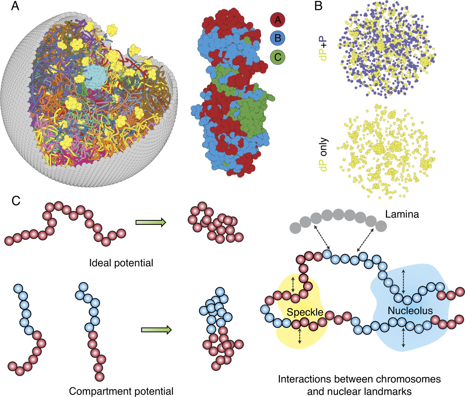
Computer model of the human nucleus for structural and dynamical characterizations.

(A) 3D rendering of the nucleus model with particle-based representations for the 46 chromosomes shown as ribbons, the nuclear lamina (gray), nucleoli (cyan), and speckles (yellow). As shown on the right, chromosomes are modeled as beads-on-a-string polymers at a 100 KB resolution, with the beads further categorized into compartment A (red), compartment B (light blue), or centromeric regions (green). (B) Speckle particles undergo chemical modifications concurrent to their spatial dynamics, and the de-phosphorylated (dP) particles contribute to droplet formation. (C) Illustration of the ideal and compartment potential that promotes chromosome compaction and microphase separation. Specific interactions between chromosomes and nuclear landmarks are shown on the right.

Figure 2 with 1 supplement

Download asset Open asset

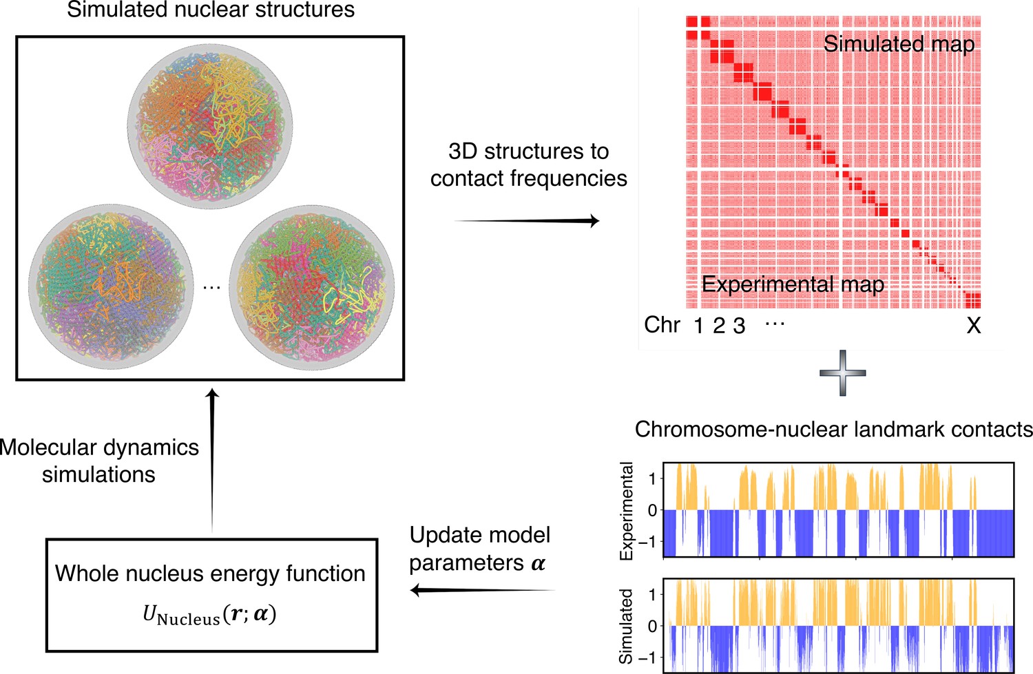
Overview of the iterative algorithm for parameterizing the nucleus model with experimental data.

Starting from an initial set of parameters, we perform molecular dynamics (MD) simulations to produce an ensemble of nuclear structures. These structures can be transformed into contacts between chromosomes or between chromosomes and nuclear landmarks for direct comparison with experimental data. Differences between simulated and experiment contacts are used to update parameters for additional rounds of optimization if needed.

Figure 2—figure supplement 1

Download asset Open asset

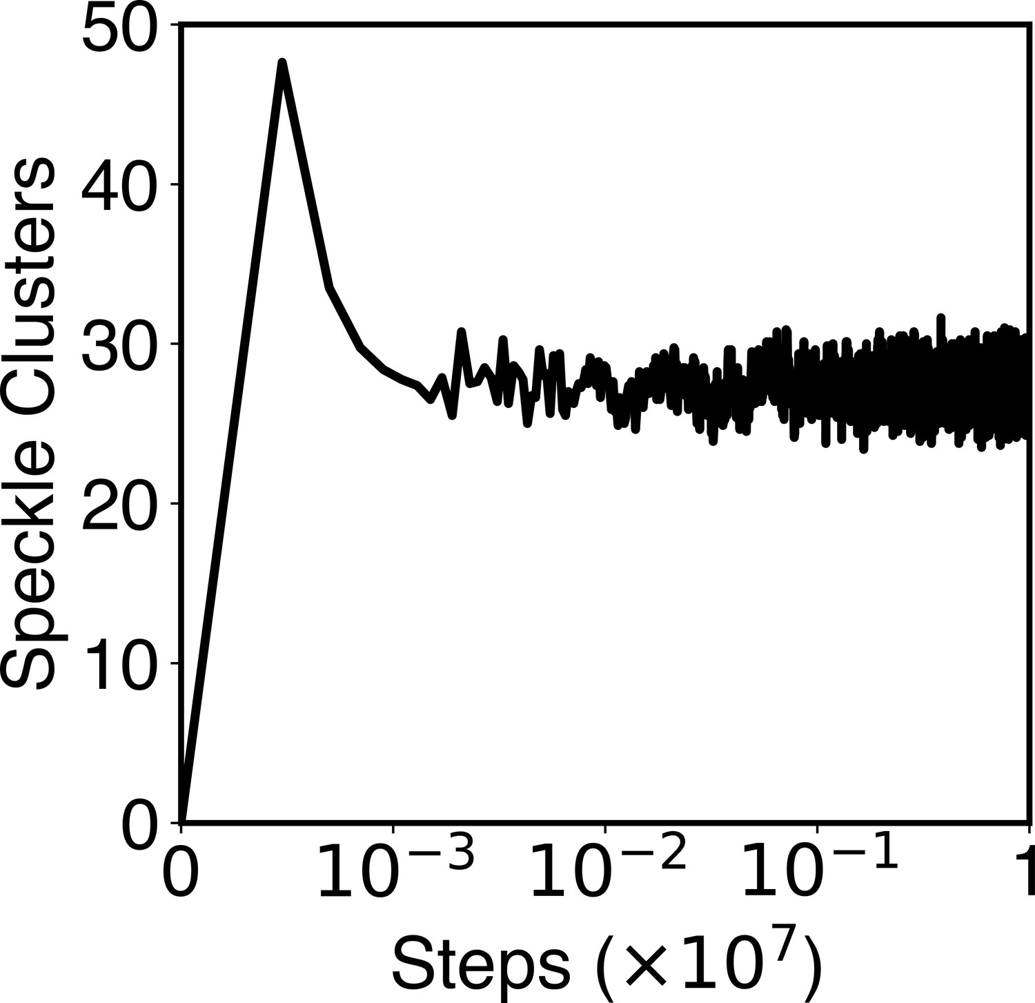
The number of speckle clusters formed along a typical simulation trajectory.

This plot shows that the kinetic scheme of speckle particle exchange produces a total of ~30 speckle droplets, reproducing experimental observations. See Appendix 1, section ‘Speckles as phase-separated droplets undergoing chemical modifications’ for more details of the kinetic scheme.

Figure 3

Download asset Open asset

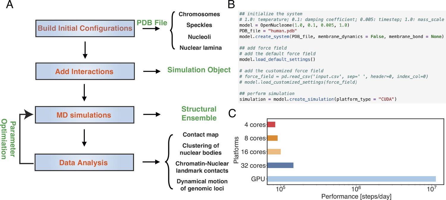
OpenNucleome facilitates GPU-accelerated simulations of the human nucleus.

(A) Illustration of workflow for setting up, performing, and analyzing molecular dynamics (MD) simulations. (B) Python scripts setting up whole nucleus simulations. (C) Performance of MD simulations on different number of CPU cores and a single GPU.

Figure 4 with 1 supplement

Download asset Open asset

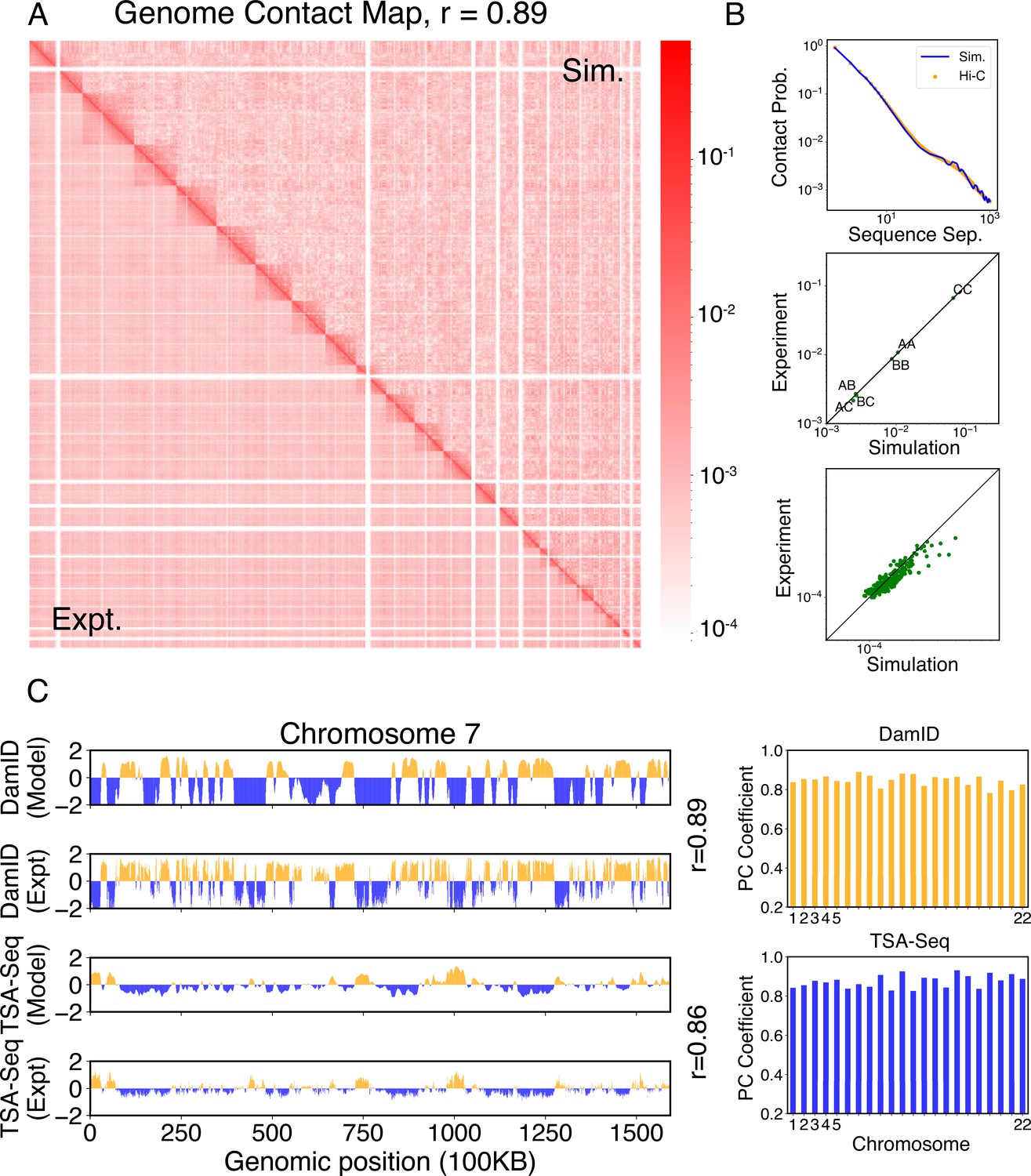
Simulated structures reproduce contact frequencies between chromosomes and between chromosomes and nuclear landmarks.

(A) Comparison between simulated (top right) and experimental (bottom left) whole-genome contact probability maps with Pearson correlation coefficient r = 0.89. Zoom-ins of various regions are provided in Figure 4—figure supplement 1. (B) Comparison between simulated and experimental average contact frequencies, including average contacts between genomic loci from the same chromosomes at a given separation (top), average contacts between genomic loci classified into different compartment types (middle), and average contacts between various chromosome pairs (bottom). (C) Comparison between simulated and experimental Lamin-B DamID (top) and SON TSA-Seq signals (bottom), with Pearson correlation coefficients of haploid chromosomes shown on the right.

Figure 4—figure supplement 1

Download asset Open asset

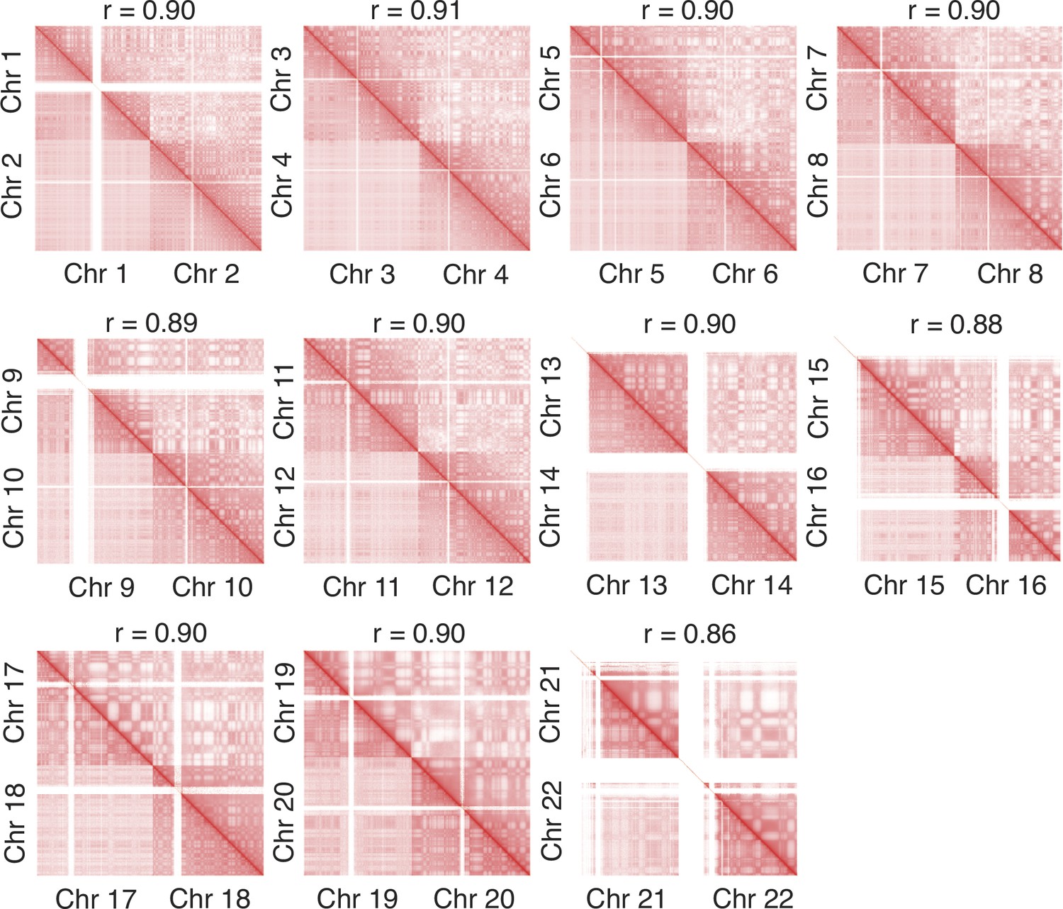
Zoom-in of various regions in the contact map presented in Figure 4 further supports the agreement between simulation and experiment.

The simulated and experimental contacts are shown in the upper and lower triangles, respectively, and the Pearson correlation coefficients r between two the sets of contacts were calculated with Equation 41.

Figure 5

Download asset Open asset

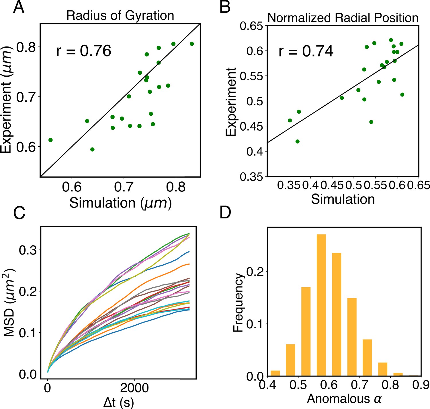
Structural and dynamical predictions of the nucleus model match results from microscopy imaging.

(A) Comparison between the simulated and experimental radius of gyration, $R_{g}$ , for haploid chromosomes. The Pearson correlation coefficient between the two, r, is shown in the legend. (B) Comparison between the simulated and experimental normalized radial positions for haploid chromosomes, with their Pearson correlation coefficient shown in the legend. Detailed definition of the normalized radial positions is provided in Appendix 1, section ‘Computing simulated normalized chromosome radial positions’. (C) Mean-squared displacements (MSDs) as a function of time are shown for selected telomeres. (D) The probability distribution of the anomalous exponent, α, obtained from fitting the MSDs curves for all telomeres with the expression, $⟨ r^{2} (Δ t) ⟩ = D_{α} Δ t^{α}$ .

Figure 6 with 2 supplements

Download asset Open asset

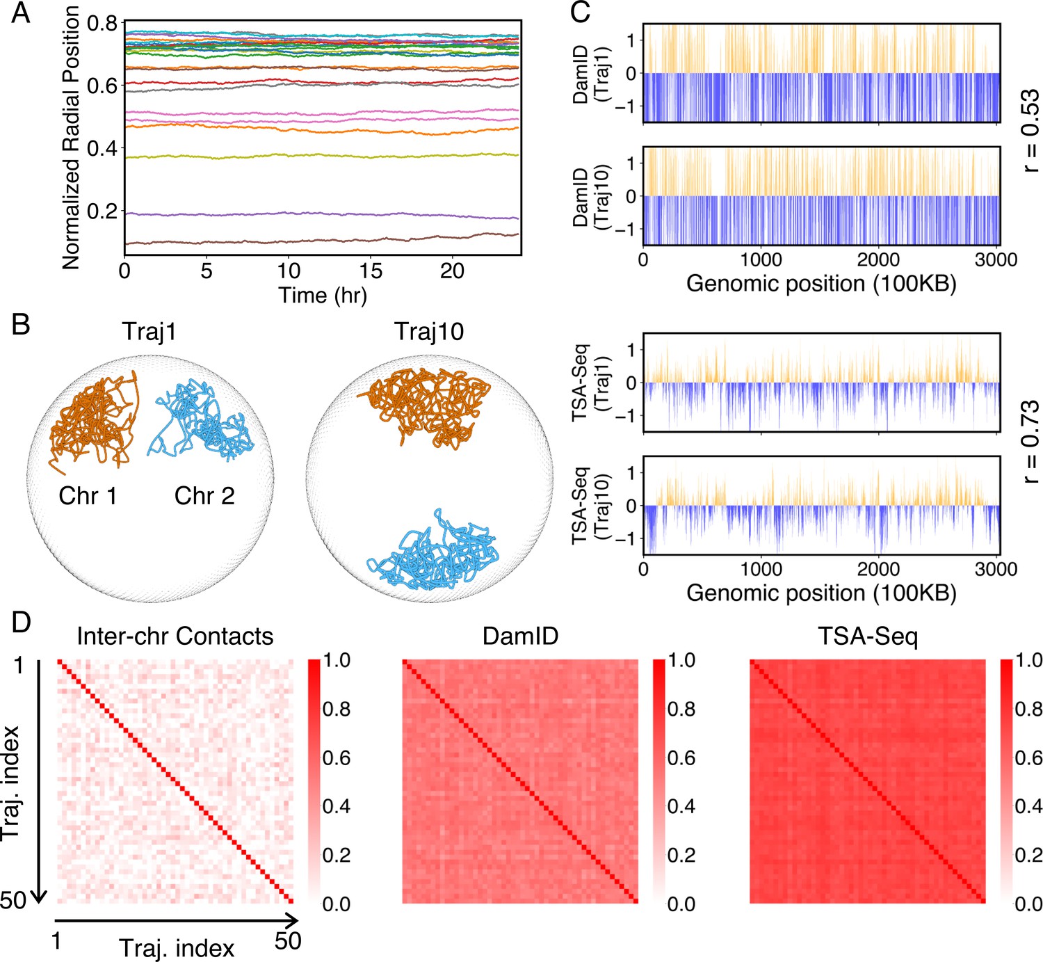
Heterogeneity and conserved features of nuclear organizations.

(A) Normalized chromosome radial positions as a function of simulation time. (B) Contacts between chromosomes 1 and 2 from two independent simulation trajectories show significant variations. (C) Genome-wide in silico Lamin B DamID (top) and SON TSA-Seq (bottom) profiles computed from two independent trajectories. Pearson correlation coefficients, r, are provided on each plot. (D) Pairwise Person correlation coefficients between interchromosomal contact matrices (left), genome-wide Lamin B DamID profiles (middle), and genome-wide SON TSA-Seq profiles (right) determined from independent trajectories. The averages excluding the diagonals of the three datasets are 0.06, 0.53, and 0.72.

Figure 6—figure supplement 1

Download asset Open asset

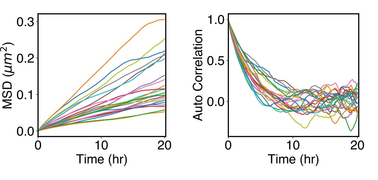
Arrested kinetics of chromosome positions over the timescale of cell cycles.

(A) Mean-squared displacement (MSD) of chromosome center of masses as a function of time. The MSDs are much smaller than the average size of chromosomes (see Rg values in Figure 5A), supporting arrested dynamics. (B) Autocorrelation function of normalized chromosome radial positions as a function of time. The autocorrelation function was computed as $C (Δ t) = \frac{\sum_{t = 1}^{N} (r_{t} - \bar{r}) (r_{t + Δ t} - \bar{r})}{\sum_{t = 1}^{N} {(r_{t} - \bar{r})}^{2}},$ where t indexes over the trajectory frames and $\bar{r}$ is the mean position.

Figure 6—figure supplement 2

Download asset Open asset

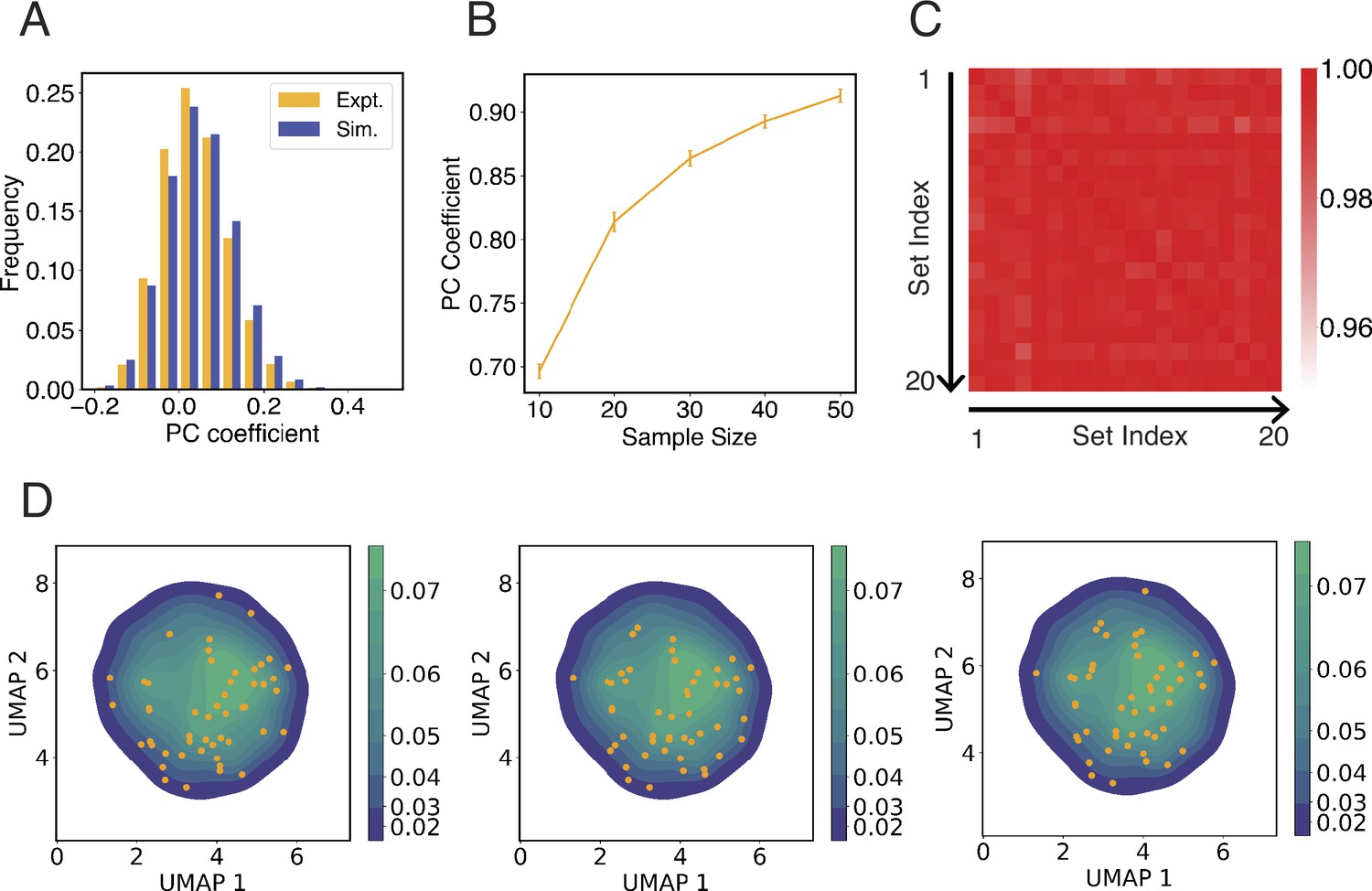
Configurations used to initialize simulations capture the heterogeneity in interchromosomal contacts seen in DNA-MERFISH data.

(A) Comparison between the simulated and experimental distribution of Pearson correlation coefficients of interchromosomal contacts. Both distributions were computed using the pairwise correlations between genome structures from the respective configurational ensemble. The pairwise interchromosomal contacts include all unique haploid pairs and were computed by averaging the contact probabilities between all genomic segments from the four respective chromosomes. The simulated configuration ensemble includes 1000 unique structures prepared following the protocol outlined in Appendix 1, section ‘Initial configurations for simulations’. The experimental ensemble includes 5455 structures reported in Su et al., 2020 using DNA-MERFISH. (B) Pearson correlation coefficient between average experimental and simulated pairwise interchromosomal contacts as a function of the number of independent configurations used to initialize simulations. Interchromosomal contacts are similarly defined as in (A) and were computed by averaging over all configurations in the respective ensembles. To compute simulated interchromosomal contacts, we used a selection procedure as detailed in Appendix 1, section ‘Initial configurations for simulations’ to determine an ensemble of a given sample size. As the size of the ensemble increases, the resulting average interchromosomal contacts agree better with experimental results. The error bars represent standard deviation computed from 20 independent trials. (**C, D**) The protocol for selecting initial configurations for simulations robustly capture the heterogeneity seen in experimental configurational ensemble. To examine the experimental structural heterogeneity, we applied Uniform Manifold Approximation and Projection (UMAP) to reduce the interchromosomal contacts into two variables following the procedure detailed in Appendix 1, section ‘Interchromosomal contacts from DNA MERFISH data’. The plot in (C) shows the Pearson correlation coefficients of 50 initial configurations represented in the UMAP variables between independent trials. The average correlation coefficient is 0.98. In (D), we show three independent initial configurations (orange dots) over the distribution of UMAP variables estimated using the experimental configurational ensemble.

Figure 7 with 1 supplement

Download asset Open asset

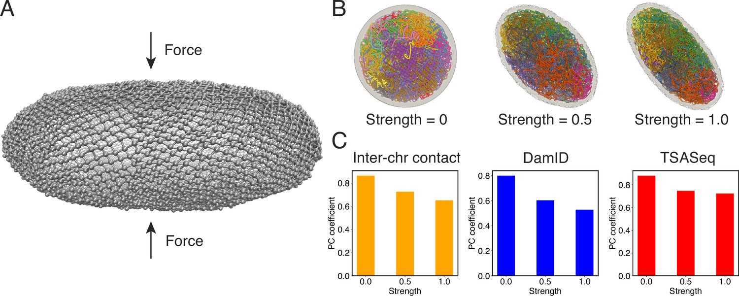
Nuclear deformations influence genome organization while preserving chromatin-speckle contacts.

(A) Illustration of force-induced nuclear envelope deformation. The nuclear lamina is modeled as a particle mesh where neighboring lamina particles are covalently bonded together. (B) Example nucleus conformations at different strengths of applied force. (C) Pearson correlation coefficients between results from simulations of deformed nuclei and those from a spherical nucleus for interchromosomal contacts (left), DamID profiles (middle), and TSA-Seq (right). The values at zero force were computed from two independent simulations starting from the same initial configurations.

Figure 7—figure supplement 1

Download asset Open asset

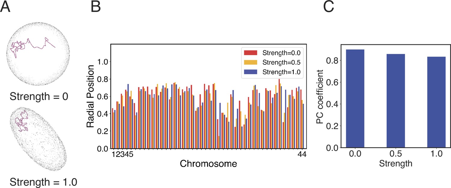
Impact of nuclear deformation on normalized chromosome radial positions.

(A) The position of chromosome 21 before and after the nuclear deformation. (B) Normalized radial positions of individual diploid chromosomes at various strengths of nuclear deformation forces. (C) Pearson correlation coefficients between normalized chromosome radial positions from simulations of deformed nuclei and those from a spherical nucleus. See Appendix 1, section ‘Nuclear envelope deformation simulations’ for simulation details.

Appendix 1—figure 1

Download asset Open asset

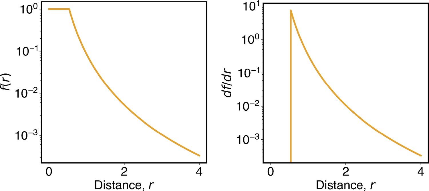
The function defined in Equation 13 smoothly switches from high to low contact probabilities.

The left and right panels plot the function and its derivative as a function of the distance, r.

Appendix 1—figure 2

Download asset Open asset

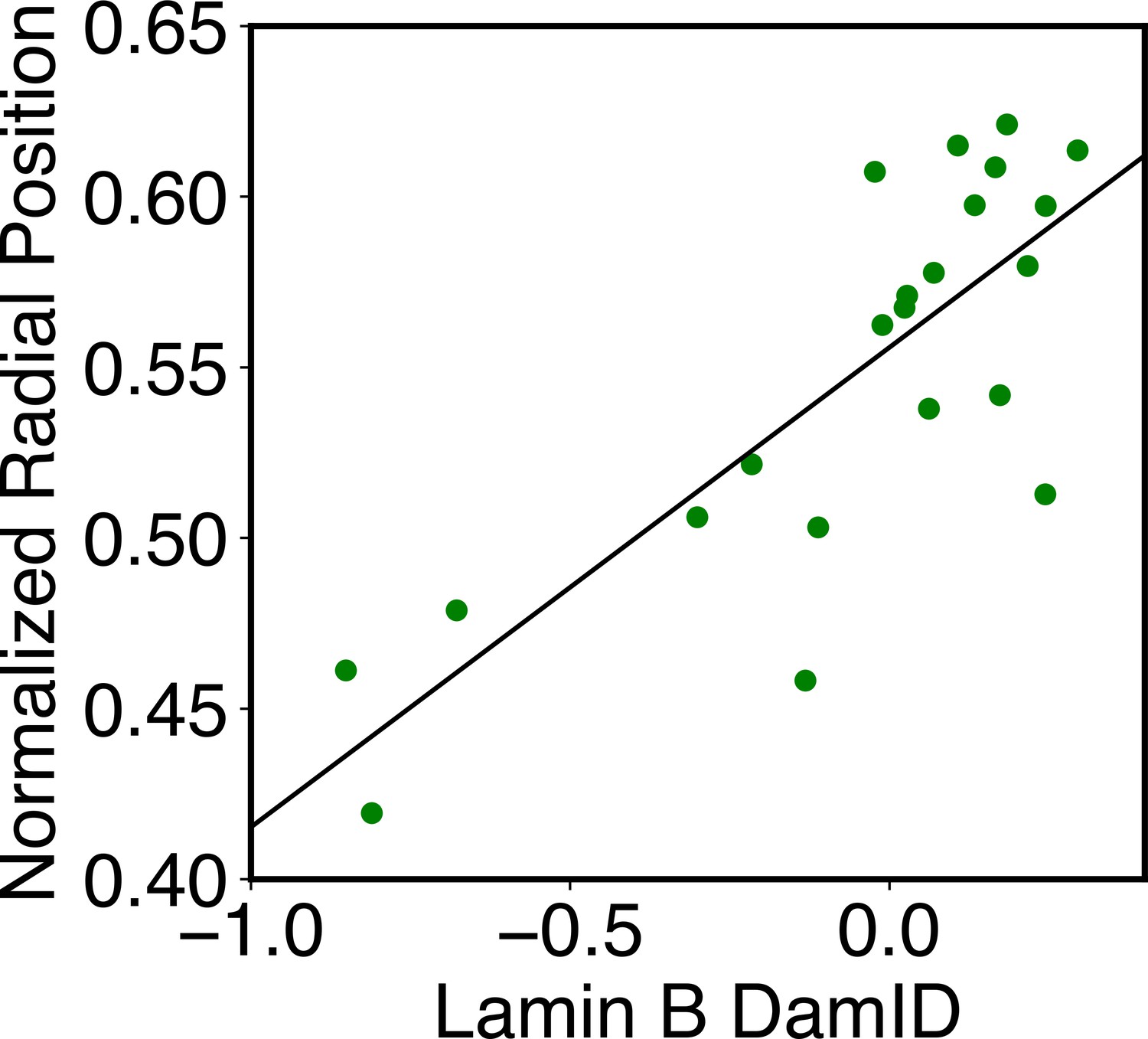
Correlation between average DamID profiles of individual chromosomes with their normalized radial positions.

The normalized radial positions were determined using the average value of all cells reported from DNA MERFISH data (Su et al., 2020). The correlation coefficient between the two datasets is 0.8.

Appendix 1—figure 3

Download asset Open asset

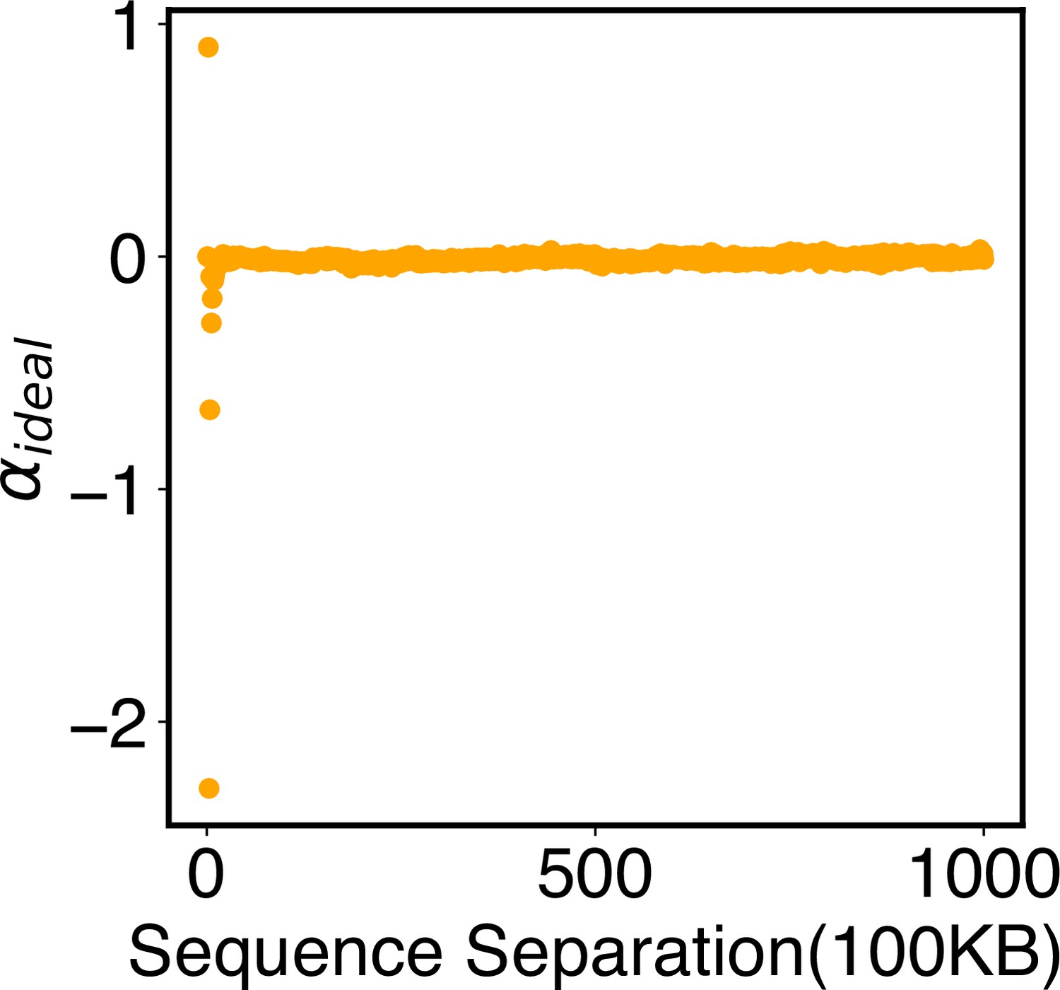
Parameters of the ideal potential, $α_{ideal}$ , as defined in Equation 12.

Numerical values for $α_{ideal}$ are included in the software’s GitHub repository.

Appendix 1—figure 4

Download asset Open asset

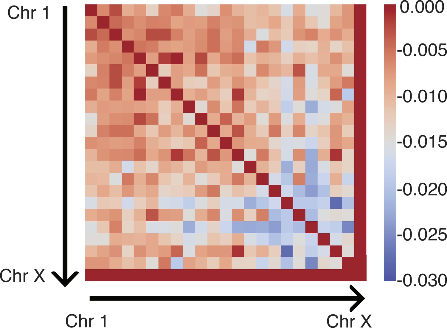
Parameters of the inter potential, $α_{inter}$ , as defined in Equation 15.

Numerical values for $α_{inter}$ are included in the software’s GitHub repository.

Appendix 1—figure 5

Download asset Open asset

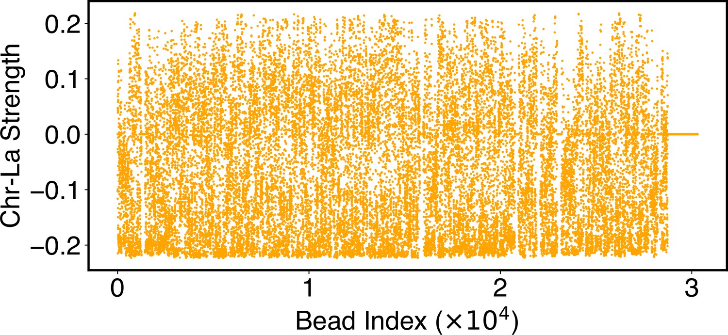
Parameters of the chromosome-lamina potential, $α^{C - L a}$ , as defined in Equation 24.

Numerical values for $α^{C - L a}$ are included in the software’s GitHub repository.

Appendix 1—figure 6

Download asset Open asset

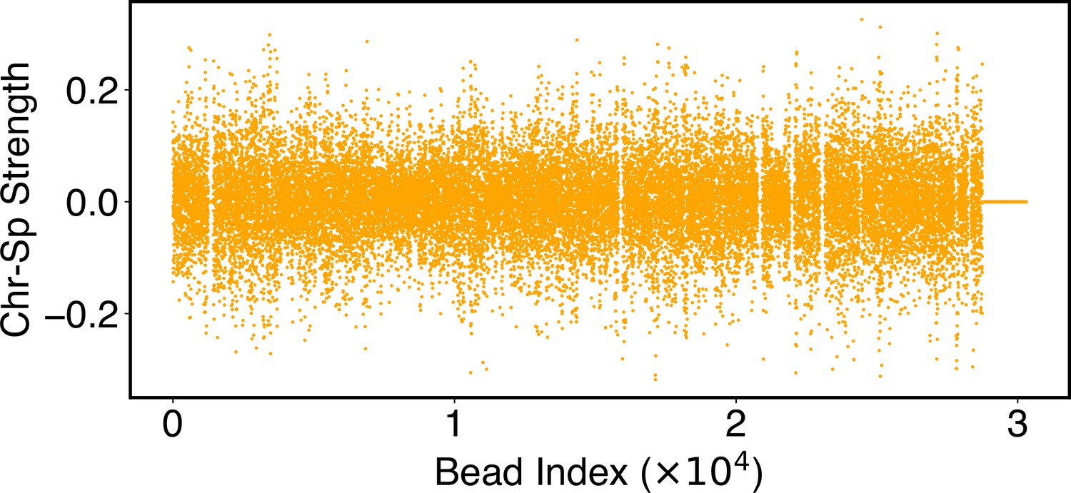
Parameters of the chromosome-lamina potential, $α^{C - S p}$ , as defined in Equation 25.

Numerical values for $α^{C - S p}$ are included in the software’s GitHub repository.

Appendix 1—figure 7

Download asset Open asset

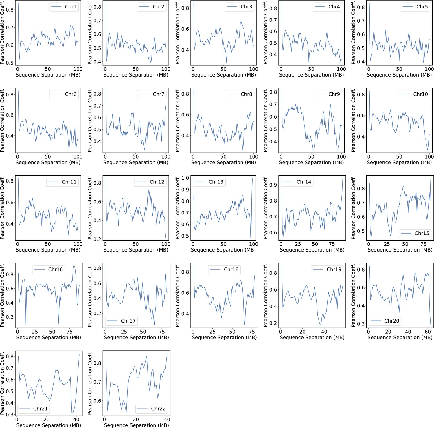
Pearson correlation coefficients between experimental and simulated contact probabilities at various sequence separations within specific chromosomes.

For each chromosome, we first gathered a set of experimental contacts alongside a matching set of simulated ones for genomic pairs within a particular separation range. The Pearson correlation coefficient at the corresponding sequence separation was then determined using Equation 41. We limited the calculations to half of the chromosome length to ensure the availability of sufficient data.

Author response image 1

Download asset Open asset

Comparison between the Class2 potential (defined in Eq. 17) and the Harmonic potential (K(r − r0)2, with K = 20 and r0 = 0.5).

Author response image 2

Download asset Open asset

Pearson correlation coefficient between experimental and simulated contact probabilities as a function of the sequence separation within specific chromosomes.

For each chromosome, we first gathered a set of experimental contacts alongside a matching set of simulated ones for genomic pairs within a particular separation range. The Pearson correlation coefficient at the corresponding sequence separation was then determined using Equation R4. We limited the calculations to half of the chromosome length to ensure the availability of sufficient data.

Tables

Appendix 1—table 1

Summary of the various terms of the chromosome energy function and the algorithms used for parameter optimization.

See also Appendix 1, section ‘Hi-C inspired interactions for the diploid human genome’ for detailed expression of the energy function and ‘Adam optimizer for chromosome interaction parameters’ for details on the optimization algorithm.

Potentials	Functional forms	Parameter values
Bonding potential	$u_{bond} (r_{i, i + 1})$ in Equation 9	Standard values in coarse-grained polymer models
Angular Potential	$u_{angle} ({\vec{r}}_{i, i + 1}, {\vec{r}}_{i + 1, i + 2})$ in Equation 9	Standard values in coarse-grained polymer models
Soft-core potential	$u_{s c} (r_{i j})$ in Equation 11	Standard values in coarse-grained polymer models
Ideal potential	$U_{i d e a l} (r)$ in Equation 12	Values for $α_{ideal}$ were obtained from optimizations against Hi-C data (see Appendix 1—figure 3).
Compartment potential	$U_{c o m p t} (r)$ in Equation 14	Values for $α_{compt}$ were obtained from optimizations against Hi-C data (see Appendix 1—table 2)
Inter potential	$U_{i n t e r} (r)$ in Equation 15	Values for $α_{inter}$ were obtained from optimizations against Hi-C data (see Appendix 1—figure 4)

Appendix 1—table 2

Summary of interaction parameters between various compartment types, that is, $α_{compt}$ defined in Equation 14.

α_AA	–0.074185
α_AB	0.112285
α_AC	0.009947
α_BB	0.059981
α_BC	0.072481
α_CC	0.088825

Appendix 1—table 3

Summary of the interaction potentials among particles that make up the nuclear landmarks and their corresponding parameter values.

See also Appendix 1, section ‘Nuclear landmark–nuclear landmark interactions’ for further discussion and ‘Unit conversion’ for choosing the size of various particles, from which the $σ_{LJ}$ were derived with a linear combination rule.

Potentials	Function forms	Parameter values
Nucleolus/nucleolus	$U_{LJ} (r_{i j})$ in Equation 18	$ϵ_{LJ} = 3.0$ and $r_{cut} = 1.5$ were chosen to mimic short-range attractions that produce an average of two nucleoli per cell. $σ_{LJ} = σ_{No} = 0.5$ .
Sp-dP/Sp-dP (speckles)	$U_{LJ} (r_{i j})$ in Equation 18	$ϵ_{LJ} = 3.0$ and $r_{cut} = 1.5$ were chosen to mimic short-range attractions that produce around 30 speckle droplets. $σ_{LJ} = σ_{Sp-dP} = 0.5$ .
Sp-dP/Sp-P (speckles)	$U_{LJ} (r_{i j})$ in Equation 18	$ϵ_{LJ} = 1.0$ and $r_{cut} = 0.5 \times 2^{1 / 6}$ were chosen as standard values to provide the excluded volume effect. $σ_{LJ} = \frac{σ_{Sp-dP} + σ_{Sp-P}}{2} = 0.5$ .
Sp-P/Sp-P (speckles)	$U_{LJ} (r_{i j})$ in Equation 18	$ϵ_{LJ} = 1.0$ and $r_{cut} = 0.5 \times 2^{1 / 6}$ were chosen as standard values to provide the excluded volume effect. $σ_{LJ} = σ_{Sp-P} = 0.5$ .
Nucleolus/speckle	$U_{LJ} (r_{i j})$ in Equation 18	$ϵ_{LJ} = 1.0$ and $r_{cut} = 0.5 \times 2^{1 / 6}$ were chosen as standard values to provide the excluded volume effect. $σ_{LJ} = \frac{σ_{No} + σ_{Sp}}{2} = 0.5$ .
Nucleolus/lamina	$U_{LJ} (r_{i j})$ in Equation 18	$ϵ_{LJ} = 1.0$ and $r_{cut} = 0.75 \times 2^{1 / 6}$ were chosen as standard values to provide the excluded volume effect. $σ_{LJ} = \frac{σ_{No} + σ_{La}^{*}}{2} = 0.75$ .
Speckle/lamina	$U_{LJ} (r_{i j})$ in Equation 18	$ϵ_{LJ} = 1.0$ and $r_{cut} = 0.75 \times 2^{1 / 6}$ were chosen as standard values to provide the excluded volume effect. $σ_{LJ} = \frac{σ_{Sp} + σ_{La}^{*}}{2} = 0.75$ .
Lamina/lamina	$U_{LJ} (r_{i j})$ in Equation 18	$ϵ_{LJ} = 1.0$ and $r_{cut} = 0.5 \times 2^{1 / 6}$ were chosen as standard values to provide the excluded volume effect. $σ_{LJ} = σ_{La} = 0.5$ .

* As mentioned in Appendix 1, section ‘Mapping lamina bead size to real unit’, a larger value for $σ_{La}$ was used here to provide a stronger excluded volume effect that prevents these particles from crossing the nucleus boundary or getting stuck in the space of the lamina particle mesh grid.

Appendix 1—table 4

Summary of the interaction potentials between chromatin particles and nuclear landmarks and their corresponding parameter values.

See also Appendix 1, section ‘Chromosome–nuclear landmark interactions’ for further discussion and ‘Adam optimizer for chromosome–nuclear body interaction parameters’ for details on the optimization algorithm.

Potentials	Functional forms	Parameter values
Chromatin-nucleolus	$U_{C-No} (r_{i j})$ in Equation 26	$η = 4.0$ provides a smooth transition in the tanh function for contacts. $r_{c} = 0.75$ reflects the minimal distances between chromatin and nucleolus beads as reflected in the excluded volume potential defined in Appendix 1—table 3. The interaction strength of the ith chromatin bead $α_{i}^{C-No} = P_{i}^{N}$ , where $P_{i}^{N}$ is the probability for the chromatin bead i to contact nucleoli as quantified by the software SPIN (Wang et al., 2021).
Chromatin-speckle	$U_{C-Sp} (r_{i j})$ in Equation 25	$η = 4.0$ and $r_{c} = 0.75$ were similarly determined as in $U_{C-No} (r_{i j})$ . Value for the interaction strength of the ith chromatin bead $α_{i}^{C-No}$ was obtained from optimizations against SON TSA-Seq data.
Chromatin-lamina	$U_{C-La} (r_{i j})$ in Equation 24	$η = 4.0$ and $r_{c} = 0.75$ were similarly determined as in $U_{C-No} (r_{i j})$ . Value for the interaction strength of the ith chromatin bead $α_{i}^{C-No}$ was obtained from optimizations against Lamin B DamID data. The extra Lennard Jones potential was included to provide the excluded volume effect, with $ϵ_{LJ} = 1.0$ and $r_{cut} = 0.75 \times 2^{1 / 6}$ as standard values. $σ_{LJ} = \frac{σ_{C} + σ_{La}^{*}}{2} = 0.75$ .

* As mentioned in Appendix 1, section ‘Mapping lamina bead size to real unit’, a larger value for $σ_{La}$ was used here to provide a stronger excluded volume effect that prevents these particles from crossing the nucleus boundary or getting stuck in the space of the lamina particle mesh grid.

Additional files

MDAR checklist: https://cdn.elifesciences.org/articles/93223/elife-93223-mdarchecklist1-v1.pdf
Download elife-93223-mdarchecklist1-v1.pdf

Download links

A two-part list of links to download the article, or parts of the article, in various formats.

Downloads (link to download the article as PDF)

Open citations (links to open the citations from this article in various online reference manager services)

Mendeley

Cite this article (links to download the citations from this article in formats compatible with various reference manager tools)

Zhuohan Lao
Kartik D Kamat
Zhongling Jiang
Bin Zhang

(2024)

OpenNucleome for high-resolution nuclear structural and dynamical modeling

eLife 13:RP93223.

https://doi.org/10.7554/eLife.93223.3

Share this article

Cite this article

Computer model of the human nucleus for structural and dynamical characterizations.

Overview of the iterative algorithm for parameterizing the nucleus model with experimental data.

The number of speckle clusters formed along a typical simulation trajectory.

OpenNucleome facilitates GPU-accelerated simulations of the human nucleus.

Simulated structures reproduce contact frequencies between chromosomes and between chromosomes and nuclear landmarks.

Zoom-in of various regions in the contact map presented in Figure 4 further supports the agreement between simulation and experiment.

Structural and dynamical predictions of the nucleus model match results from microscopy imaging.

Heterogeneity and conserved features of nuclear organizations.

Arrested kinetics of chromosome positions over the timescale of cell cycles.

Configurations used to initialize simulations capture the heterogeneity in interchromosomal contacts seen in DNA-MERFISH data.

Nuclear deformations influence genome organization while preserving chromatin-speckle contacts.

Impact of nuclear deformation on normalized chromosome radial positions.

The function defined in Equation 13 smoothly switches from high to low contact probabilities.

Correlation between average DamID profiles of individual chromosomes with their normalized radial positions.

Parameters of the ideal potential, αideal, as defined in Equation 12.

Parameters of the inter potential, αinter, as defined in Equation 15.

Parameters of the chromosome-lamina potential, αC−La, as defined in Equation 24.

Parameters of the chromosome-lamina potential, αC−Sp, as defined in Equation 25.

Pearson correlation coefficients between experimental and simulated contact probabilities at various sequence separations within specific chromosomes.

Comparison between the Class2 potential (defined in Eq. 17) and the Harmonic potential (K(r − r0)2, with K = 20 and r0 = 0.5).

Pearson correlation coefficient between experimental and simulated contact probabilities as a function of the sequence separation within specific chromosomes.

Summary of the various terms of the chromosome energy function and the algorithms used for parameter optimization.

Summary of interaction parameters between various compartment types, that is, αcompt defined in Equation 14.

Summary of the interaction potentials among particles that make up the nuclear landmarks and their corresponding parameter values.

Summary of the interaction potentials between chromatin particles and nuclear landmarks and their corresponding parameter values.

MDAR checklist

Downloads (link to download the article as PDF)

Open citations (links to open the citations from this article in various online reference manager services)

Cite this article (links to download the citations from this article in formats compatible with various reference manager tools)

Parameters of the ideal potential, $α_{ideal}$ , as defined in Equation 12.

Parameters of the inter potential, $α_{inter}$ , as defined in Equation 15.

Parameters of the chromosome-lamina potential, $α^{C - L a}$ , as defined in Equation 24.

Parameters of the chromosome-lamina potential, $α^{C - S p}$ , as defined in Equation 25.

Summary of interaction parameters between various compartment types, that is, $α_{compt}$ defined in Equation 14.