Juxtaposition of heterozygous and homozygous regions causes reciprocal crossover remodelling via interference during Arabidopsis meiosis
- University of Cambridge, United Kingdom
- Adam Mickiewicz University, Poland
- University of North Carolina at Chapel Hill, United States
- University of North Carolina School of Medicine, United States
- University of Birmingham, United Kingdom
Figures
Figure 1

Testing for crossover modification by Arabidopsis natural variation.
(A) Historical crossover frequency (red, cM/Mb) and sequence diversity (π, blue) along the physical length of the Arabidopsis thaliana chromosomes (Mb) (Cao et al., 2011; Choi et al., 2013). Mean values are indicated by horizontal dotted lines and centromeres by vertical dotted lines. The fluorescent crossover intervals analysed are indicated by solid vertical lines and coloured triangles. (B) Map showing the geographical origin of the Arabidopsis accessions studied, indicated by red points. (C) Genetic diagram illustrating the experimental approach with a single chromosome shown for simplicity. Fluorescent crossover reporters (triangles) were generated in the Col background (black) and crossed to accessions of interest (red) to generate F1 heterozygotes. Following meiosis the proportion of parental:crossover gametes from F1 heterozygotes was analysed to measure genetic distance (cM) between the fluorescent protein encoding transgenes.
Figure 2 with 1 supplement

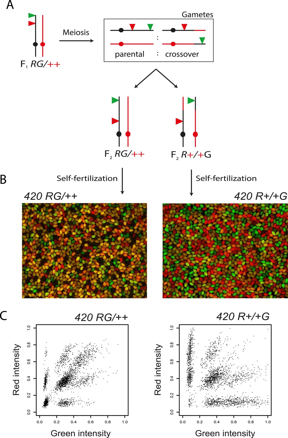
High-throughput measurement of crossover frequency using image analysis of fluorescent seed.
(A) Combined red and green, red alone and green alone fluorescent micrographs of seed from a self-fertilized 420/++ plant. (B) CellProfiler output showing identification of seed objects by green lines and scoring of red and green fluorescence shown by shading. Blue shading shows an absence of colour. (C–D) Histograms of seed object fluorescence intensities, with coloured and non-coloured seed divided by vertical dotted lines. (E) Plot of seed object red vs green fluorescence intensities, with each point representing an individual seed. The red and green dashed lines show the colour vs non-colour divisions indicated in (C–D). The formula used for cM calculation is printed below. (F) 420 cM measurements from replicate plants of the indicated genotypes (Col/Col F1, Col/Ler F1, Col/Sha F1) are shown by black dots with mean values indicated by red dots. Data generated by automatic and manual scoring are plotted alongside one another. Measurements made by the different methods were not significantly different as tested using generalized linear model (GLM). See Figure 2—source data 1.
-
Figure 2—source data 1
420 crossover frequency measured via manual or automated scoring of seed fluorescence.
- https://doi.org/10.7554/eLife.03708.008
Figure 2—figure supplement 1
Distinguishing 420 RFP-GFP/++ vs RFP-+/+-GFP recombinant individuals.
(A) Genetic diagram illustrating generation of F2 plants heterozygous for the 420 fluorescent transgenes, annotated as in Figure 1C. F2 plants heterozygous for the fluorescent transgenes can occur via fertilization with recombinant or non-recombinant chromosomes. (B) Fluorescence micrographs of seed derived from self-fertilization of 420 RFP-GFP/++ vs RFP-+/+-GFP plants. (C) Plots of seed object red vs green fluorescence intensities, with each point representing an individual seed from either self-fertilized 420 RFP-GFP/++ or RFP-+/+-GFP plants.
Figure 3
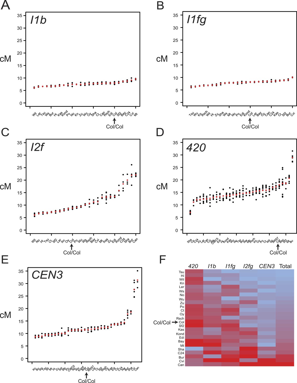
Variation in F1 hybrid crossover frequency.
(A–E) Genetic distance (cM) measurements for fluorescent crossover intervals I1b, I1fg, I2f, 420 and CEN3 with individual replicates (black dots) and mean values (red dots) for the crosses labelled on the x-axis. See Figure 3—source data 1–5. (F) Heatmap summarising crossover frequency data for F1 crosses with data from all five intervals. Accessions are listed as rows and fluorescent intervals listed as columns. The heatmap is ordered according to ascending ‘Total’ cM (red = highest, blue = lowest), which is the sum of the individual interval genetic distances. GLM testing for significant differences between total recombinant vs non-recombinant counts between replicate groups of Col-0 homozygotes and F1 heterozygotes was performed, for genotypes where data from all five tested intervals were collected (Table 3). Col/Col homozygous data are labelled and highlighted with an arrow in each plot.
-
Figure 3—source data 1
I1b F1 flow cytometry count data.
- https://doi.org/10.7554/eLife.03708.011
-
Figure 3—source data 2
I1b F1 flow cytometry count data.
- https://doi.org/10.7554/eLife.03708.012
-
Figure 3—source data 3
I1b F1 flow cytometry count data.
- https://doi.org/10.7554/eLife.03708.013
-
Figure 3—source data 4
I1b F1 flow cytometry count data.
- https://doi.org/10.7554/eLife.03708.014
-
Figure 3—source data 5
CEN3 F1 flow cytometry count data.
- https://doi.org/10.7554/eLife.03708.015
Figure 4 with 1 supplement
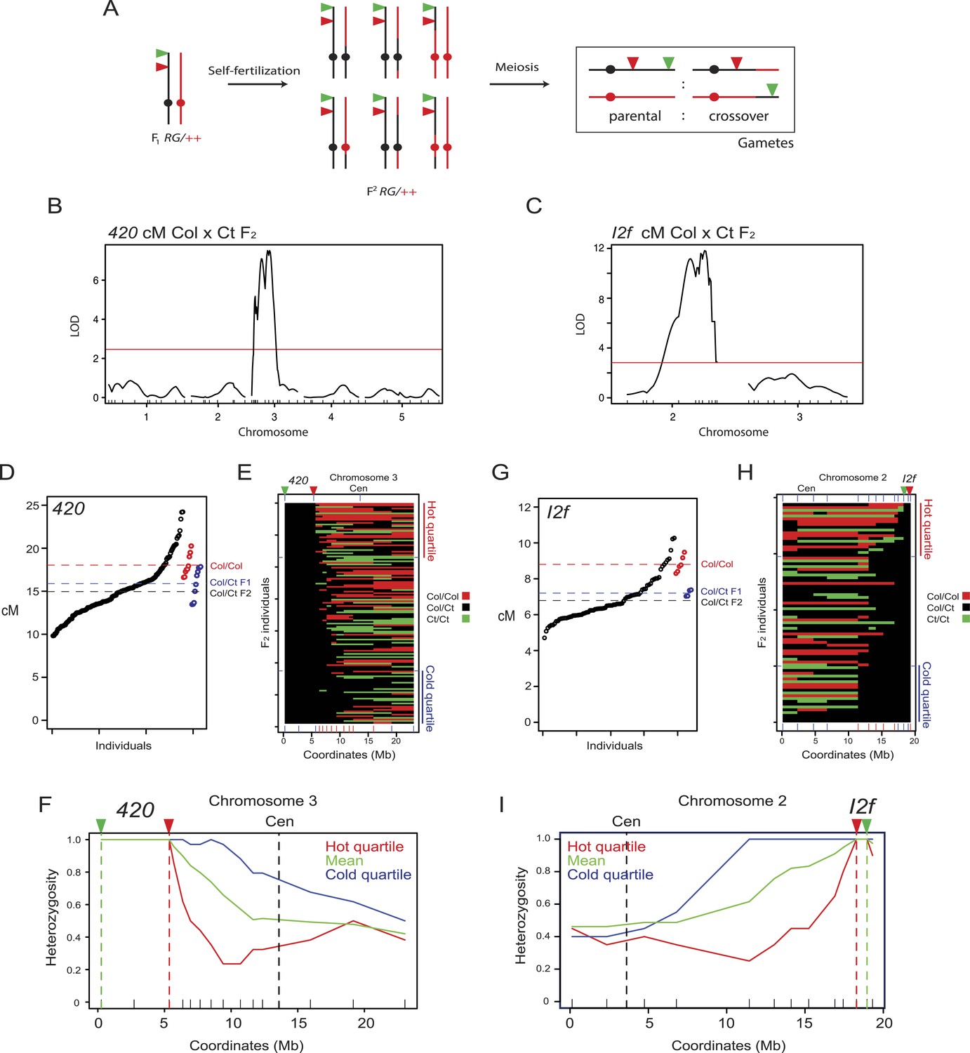
Modification of crossover frequency by juxtaposition of heterozygosity and homozygosity.
(A) Diagram illustrating chromosome 3 genotypes (black = Col, red = Ct) in RG/++ F1 individuals and their F2 progeny. A single chromosome is shown for simplicity. Gametes or progeny are analysed for patterns of fluorescence following meiosis to measure genetic distance. (B) The program Rqtl was used to test for association between Col/Ct genotypes and 420 cM in a 420/++ F2 population. The logarithm of odds (LOD) score is plotted along the 5 chromosomes with the positions of markers shown along the x-axis by ticks. The red horizontal line shows the 5% genome-wide significance threshold calculated with Hayley-Knott regression and by running 10,000 permutations. (C) As for (B) but analyzing Col/Ct markers on chromosomes 2 and 3 for an I2f/++ F2 population. (D) 420 cM measurements from Col/Ct 420/++ F2 (black), Col/Col homozygotes (red) and Col/Ct F1 (blue) individuals. Mean values are indicated by horizontal dotted lines. See Figure 4—source data 1. (E) Chromosome 3 genotypes shown for 420/++ F2 individuals ranked by crossover frequency. Each horizontal row represents a single F2 individual. X-axis ticks show marker positions, and which are coloured red when they showed significantly higher homozygosity in the hottest vs coldest quartiles (FDR-corrected chi square test). Fluorescent T-DNAs are indicated by triangles, in addition to the centromere (Cen). (F) Heterozygosity along chromosome 3 in the hottest (red), coldest (blue) 420 F2 quartiles and the mean (green). The locations of reporter T-DNAs and the centromeres are indicated by vertical dashed lines. (G–I) As for (D–F) but for interval I2f. See Figure 4—source data 2.
-
Figure 4—source data 1
420 Col/Ct F2 fluorescent seed count data.
- https://doi.org/10.7554/eLife.03708.018
-
Figure 4—source data 2
I2f Col/Ct F2 fluorescent seed count data.
- https://doi.org/10.7554/eLife.03708.019
-
Figure 4—source data 3
CEN3 Col/Ct F2 flow cytometry count data.
- https://doi.org/10.7554/eLife.03708.020
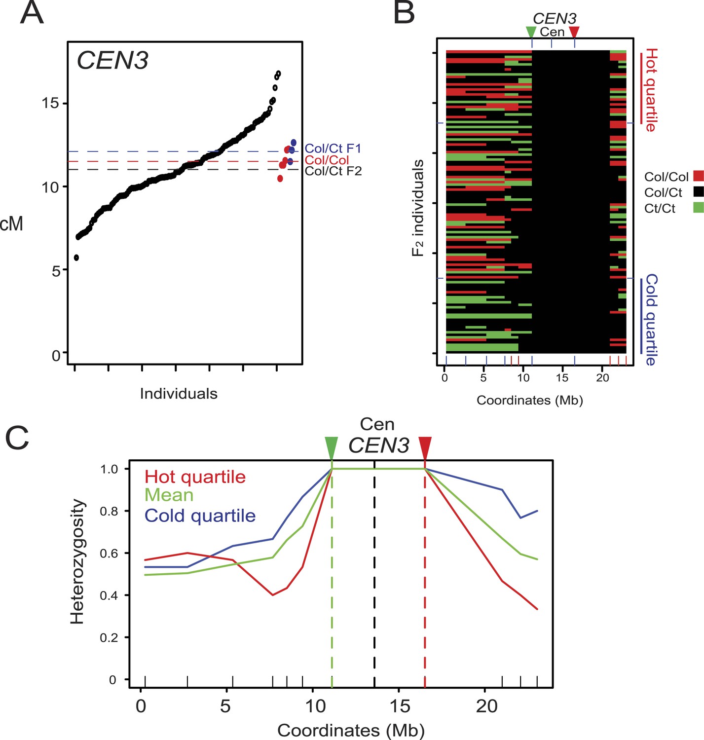
Figure 4—figure supplement 1
Modification of crossover frequency by juxtaposition of heterozygosity and homozygosity.
(A) CEN3 cM from Col/Ct CEN3/++ F2 (black), Col/Col homozygotes (red) and Col/Ct F1 (blue) individuals. Horizontal dotted lines indicate mean value. See Figure 4—source data 3. (B) Chromosome 3 genotypes shown for CEN3/++ F2 individuals ranked by crossover frequency. X-axis ticks show marker positions, and which are coloured red when they showed significantly higher homozygosity in the hottest vs coldest quartile (FDR-corrected chi square tests). Fluorescent T-DNAs are indicated by triangles, in addition to the centromere. (C) Heterozygosity along chromosome 3 in the hottest (red), coldest (blue) CEN3 F2 quartiles and the mean (green). The locations of reporter T-DNAs and the centromeres are indicated by vertical dashed lines.
Figure 5 with 1 supplement
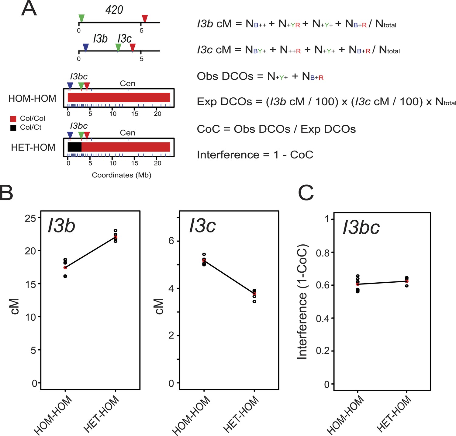
Juxtaposition of heterozygous and homozygous regions triggers reciprocal crossover remodelling.
(A) Schematic diagram illustrating the physical location of 420 and I3bc transgenes expressing fluorescent proteins in seed and pollen. Beneath are diagrams illustrating the locations of Col/Col homozygous (red) and Col/Ct heterozygous (black) regions along chromosome 3. Positions of Col/Ct genotyping markers are indicated by blue ticks along the axis of the chromosome. Printed alongside are formulae for the calculation of genetic distance (cM) and crossover interference using I3bc. Counts of pollen with different combinations of fluorescence are indicated. For example, NBYR indicates the number of pollen with blue, yellow and red fluorescence. (B) I3b and I3c genetic distance (cM) measured in HOM-HOM and HET-HOM plants as illustrated in (A). See Figure 5—source data 1. (C) As for (B) but showing calculation of crossover interference (1-CoC). See Figure 5—source data 2.
-
Figure 5—source data 1
Three colour I3bc FTL flow cytometry count data.
- https://doi.org/10.7554/eLife.03708.025
-
Figure 5—source data 2
Three colour I3bc FTL flow cytometry count data–measurement of crossover interference.
- https://doi.org/10.7554/eLife.03708.026
Figure 5—figure supplement 1
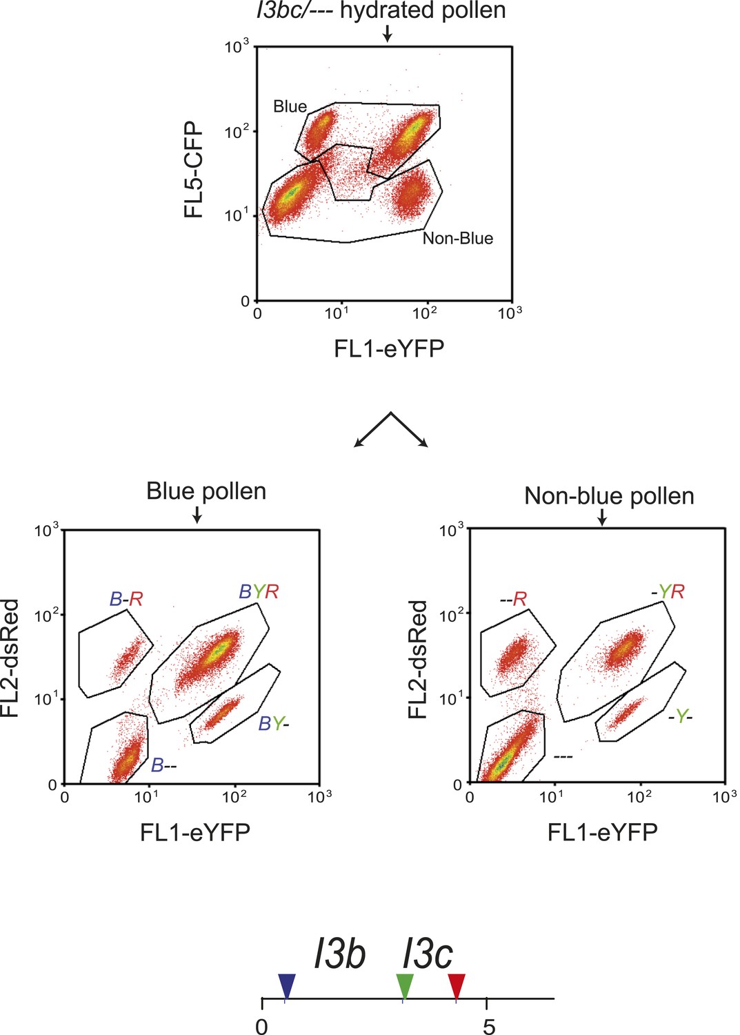
Analysis of I3bc recombination using three-colour flow cytometry.
Flow cytometry plots are shown measuring pollen for the indicated colour of fluorescent protein. In the upper plot total hydrated pollen is divided into blue and non-blue populations using polygonal gates. Gated populations are then analysed separately in the lower plots for red and yellow fluorescence. The indicated polygon gates represent the labelled pollen fluorescent classes. Beneath the plots is a diagram indicating the physical location of the I3bc T-DNA insertions at the end of chromosome 3. The T-DNAs are represented by coloured triangles.
Figure 6 with 1 supplement
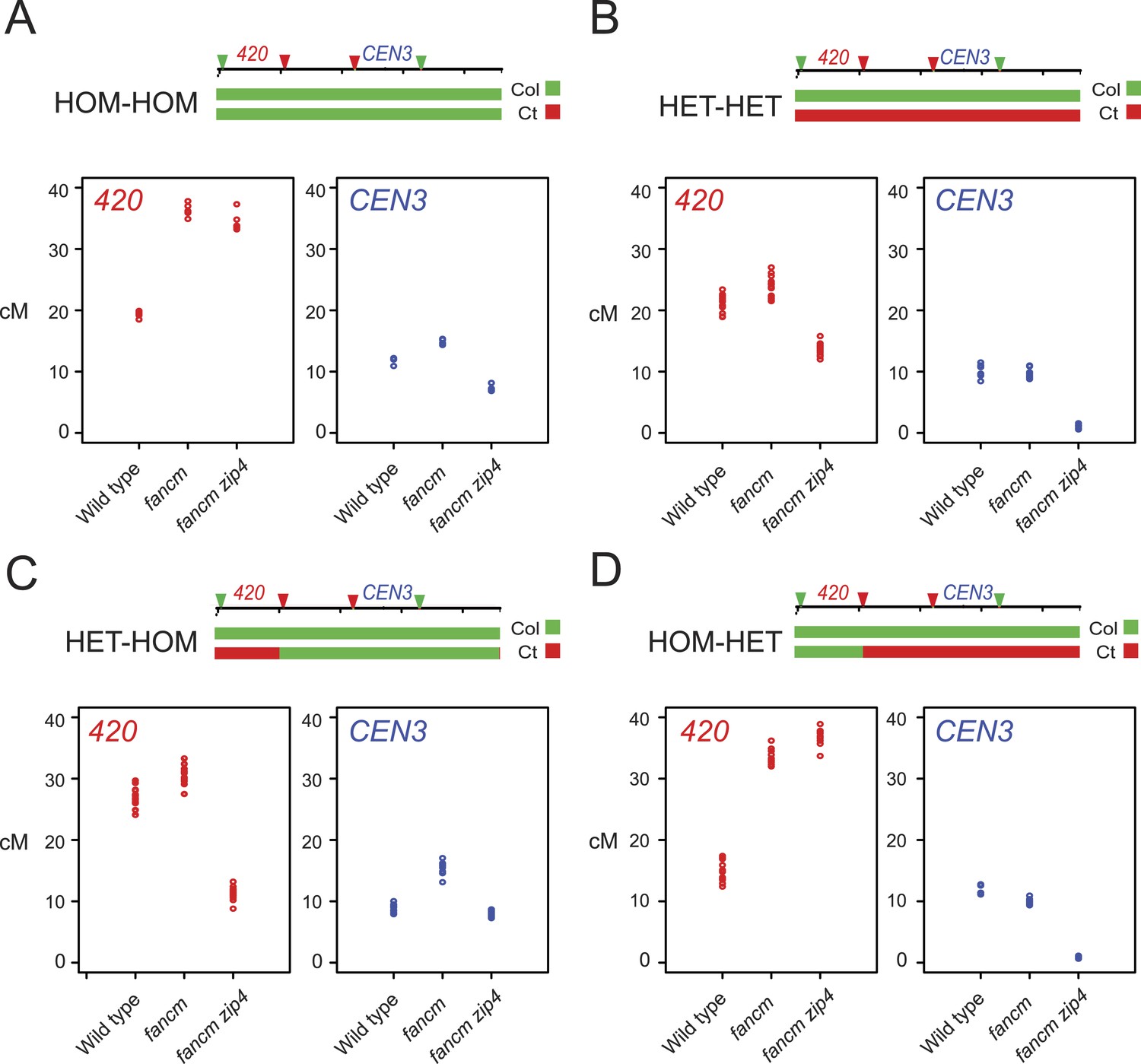
Genetic requirements of crossover remodelling via juxtaposition of heterozygous and homozygous regions.
(A–D) Replicate measurements of 420 (red) and CEN3 (blue) genetic distances (cM) are plotted in wild type, fancm and fancm zip4. See Figure 6—source data 1, 2. Chromosome 3 genotypes of the plants analysed are indicated above the plots (green = Col and red = Ct), for example, HET-HOM indicates heterozygous within 420 and homozygous outside.
-
Figure 6—source data 1
420 fluorescent seed count data from wild type, fancm and fancm zip4 individuals with varying heterozygosity.
- https://doi.org/10.7554/eLife.03708.030
-
Figure 6—source data 2
CEN3 flow cytometry count data from wild type, fancm and fancm zip4 individuals with varying heterozygosity.
- https://doi.org/10.7554/eLife.03708.031
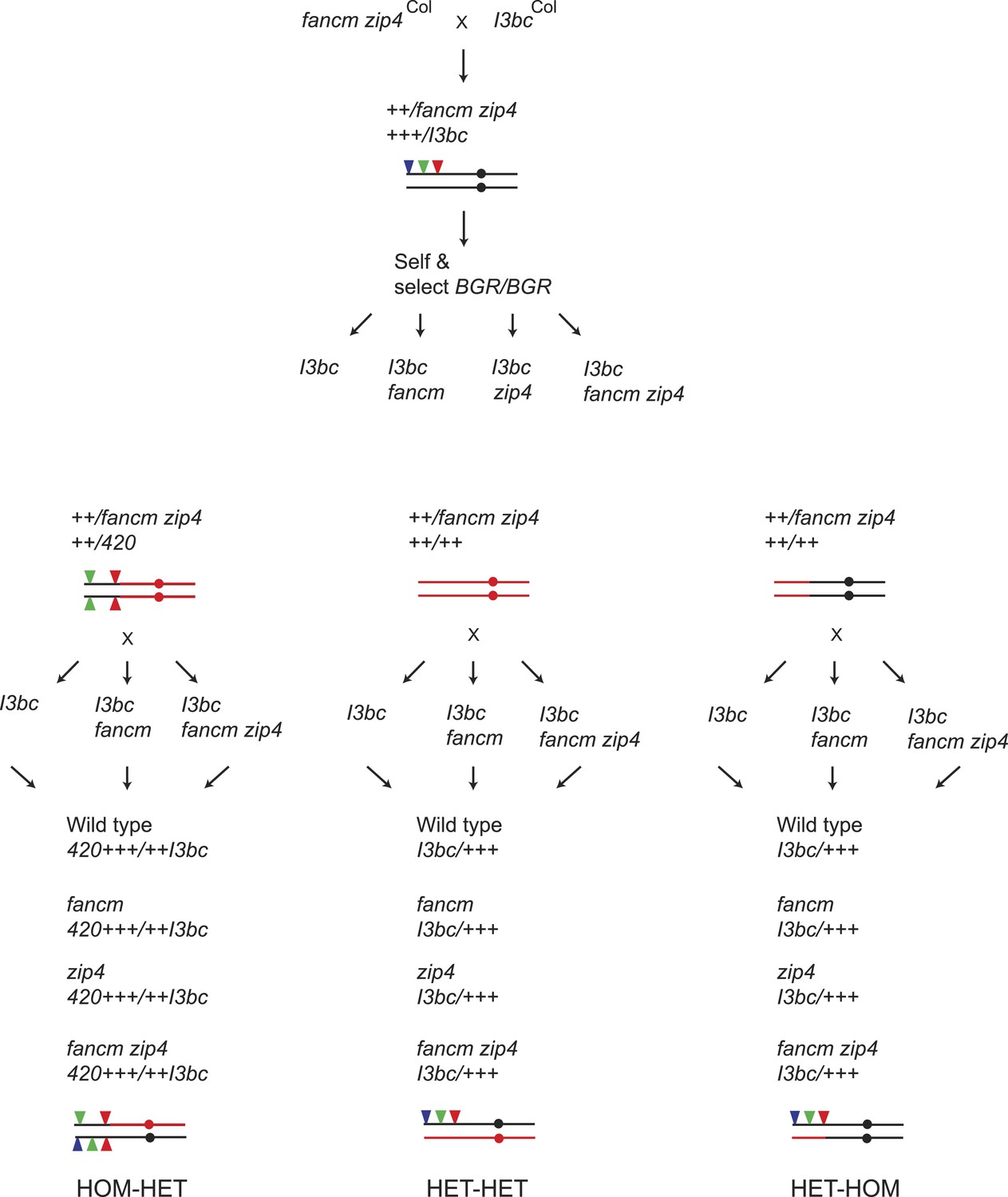
Figure 6—figure supplement 1
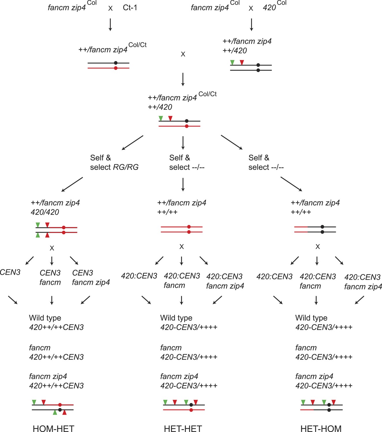
Generation of wild type, fancm or fancm zip4 420-CEN3 individuals with varying patterns of Col/Ct heterozygosity.
Diagram showing the crossing scheme used to generate plants to test the requirement of recombination pathways in crossover remodelling. At relevant points the genotype of chromosome 3 is illustrated graphically with black indicating Col and red indicating Ct. The circles represent the location of the centromere and the red and green filled triangles represent the fluorescent T-DNAs of both 420 and CEN3.
Figure 7
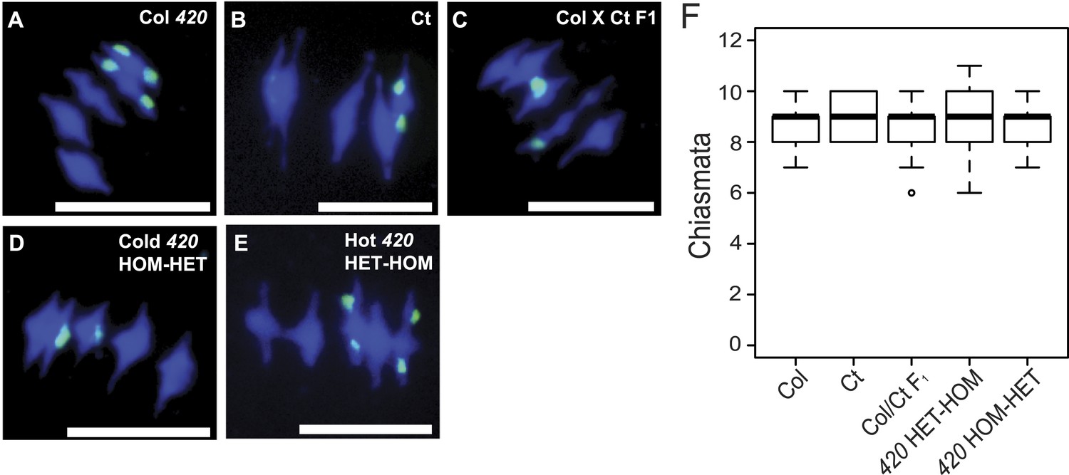
Total chiasmata frequencies are stable between Col, Ct and recombinant lines.
(A–E) Metaphase-I chromosome spreads from anthers from (A) Col/Col 420, (B) Ct/Ct, (C) Col × Ct F1, (D) a Col × Ct 420 (HOM-HET) cold recombinant line and (E) a Col × Ct 420 hot (HET-HOM) recombinant line. DNA is stained with DAPI (blue) and labelled with a 45S rDNA probe (green). Scale bars = 10 μM. (F) Boxplot showing total number of chiasmata per nucleus for each genotype. See Figure 7—source data 1.
-
Figure 7—source data 1
Chiasmata count data.
- https://doi.org/10.7554/eLife.03708.034
Figure 8 with 1 supplement

Crossover interference increases when heterozygous and homozygous regions are juxtaposed.
(A–D) Replicate measurements of I3b and I3c genetic distances (cM), and I3bc crossover interference are plotted in wild type, fancm, fancm zip4 and zip4. Black dots represent replicate measurements with mean values indicated by red dots. Chromosome 3 genotypes of the plants analysed are indicated above the plots (green = Col and red = Ct), for example, HET-HOM indicates heterozygous within I3bc and homozygous outside. See Figure 8—source data 1, 2. (E) I3b and I3c genetic distances (cM) are plotted in wild type and zip4 mutants with varying patterns of heterozygosity, labelled as for (A–D). Mean values between samples are connected with red lines. See Figure 8—source data 3, 4.
-
Figure 8—source data 1
I3bc fluorescent seed count data from wild type, fancm and fancm zip4 individuals with varying heterozygosity.
- https://doi.org/10.7554/eLife.03708.036
-
Figure 8—source data 2
Calculation of I3bc interference from wild type, fancm and fancm zip4 individuals with varying heterozygosity.
- https://doi.org/10.7554/eLife.03708.037
-
Figure 8—source data 3
I3bc fluorescent seed count data from wild type and zip4 individuals with varying heterozygosity.
- https://doi.org/10.7554/eLife.03708.038
-
Figure 8—source data 4
Calculation of I3bc interference in wild type and zip4.
- https://doi.org/10.7554/eLife.03708.039
Figure 8—figure supplement 1
Generation of wild type, fancm, zip4 or fancm zip4 I3bc/++ plants with varying patterns of Col/Ct heterozygosity.
Diagram showing the crossing scheme used to generate plants to investigate the impact of the Col/Ct heterozygosity on crossover interference. Genotypes differing in polymorphism pattern for crosses with I3bc lines were obtained as described in Figure 6—figure supplement 1. The genotype of chromosome 3 is illustrated graphically with black indicating Col and red indicating Ct. The circles represent the location of the centromere and the red and green filled triangles represent the fluorescent T-DNAs for both 420 and CEN3.
Tables
Table 1
Correlations between historical recombination and sequence diversity at varying physical scales
| Scale (π) | Chr1 | Chr2 | Chr3 | Chr4 | Chr5 |
|---|---|---|---|---|---|
| 5 kb | 0.521 | 0.301 | 0.545 | 0.575 | 0.541 |
| 10 kb | 0.556 | 0.305 | 0.565 | 0.602 | 0.562 |
| 50 kb | 0.657 | 0.381 | 0.579 | 0.692 | 0.619 |
| 100 kb | 0.699 | 0.563 | 0.601 | 0.744 | 0.646 |
| 500 kb | 0.741 | 0.528 | 0.615 | 0.841 | 0.653 |
| 1 Mb | 0.639 | 0.504 | 0.683 | 0.846 | 0.624 |
| Scale (θ) | Chr1 | Chr2 | Chr3 | Chr4 | Chr5 |
|---|---|---|---|---|---|
| 5 kb | 0.537 | 0.298 | 0.557 | 0.585 | 0.553 |
| 10 kb | 0.569 | 0.303 | 0.576 | 0.610 | 0.572 |
| 50 kb | 0.662 | 0.382 | 0.592 | 0.699 | 0.623 |
| 100 kb | 0.710 | 0.573 | 0.617 | 0.752 | 0.650 |
| 500 kb | 0.754 | 0.534 | 0.635 | 0.844 | 0.655 |
| 1 Mb | 0.647 | 0.504 | 0.697 | 0.849 | 0.635 |
-
Spearman's rank correlation between historical crossover frequency estimates from LDhat and sequence diversity (θ and π) at varying physical scales (Cao et al., 2011; Choi et al., 2013). Adjacent windows of the indicated physical size were used for correlations.
Table 2
Fluorescent crossover reporter intervals
| Interval | Chr | Method | T-DNA 1 | T-DNA 2 | Mb | Location | cM/Mb (Col-0) | cM/Mb (F1) | Heterozygosity |
|---|---|---|---|---|---|---|---|---|---|
| I1b | 1 | Pollen | 3,905,441-YFP | 5,755,618-dsRed2 | 1.85 | Interstitial | 4.25 | 4.05 | 1.93 (3.16) |
| I1c | 1 | Pollen | 5,755,618-dsRed2 | 9,850,022-CFP | 4.09 | Interstitial | 4.55 | N/A | 2.80 (3.16) |
| I1fg | 1 | Pollen | 24,645,163-YFP | 25,956,590-dsRed2 | 1.31 | Interstitial | 6.20 | 6.02 | 2.52 (3.16) |
| I2a | 2 | Pollen | 12,640,092-CFP | 13,226,013-YFP | 0.59 | Interstitial | 5.19 | N/A | 2.33 (3.30) |
| I2b | 2 | Pollen | 13,226,013-YFP | 14,675,407-dsRed2 | 1.45 | Interstitial | 3.09 | N/A | 1.53 (3.30) |
| I2f | 2 | Pollen | 18,286,716-dsRed2 | 18,957,093-YFP | 0.67 | Sub-telomeric | 13.02 | 17.41 | 1.43 (3.30) |
| 420 | 3 | Seed | 256,516-GFP | 5,361,637-dsRed2 | 5.11 | Sub-telomeric | 3.70 | 2.93 | 1.19 (3.37) |
| CEN3 | 3 | Pollen | 11,115,724-YFP | 16,520,560-dsRed2 | 5.40 | Centromeric | 2.11 | 2.38 | 6.69 (3.37) |
| I3b | 3 | Pollen | 498,916-CFP | 3,126,994-YFP | 2.63 | Sub-telomeric | 5.99 | N/A | 1.11 (3.37) |
| I3c | 3 | Pollen | 3,126,994-YFP | 4,319,513-dsRed2 | 1.19 | Sub-telomeric | 4.01 | N/A | 1.64 (3.37) |
| I5c | 5 | Pollen | 2,372,623-CFP | 3,760,756-YFP | 1.39 | Interstitial | 4.01 | N/A | 1.01 (3.27) |
| I5d | 5 | Pollen | 3,760,756-YFP | 5,497,513-dsRed2 | 1.74 | Interstitial | 3.20 | N/A | 1.56 (3.27) |
-
The interval name is listed together with chromosome, method of scoring and location of the flanking T-DNAs together with the fluorescent proteins they encode. Interval cM/Mb values from Col-0 homozygous are listed (Col-0), in addition to the mean cM/Mb observed across all F1 crosses (F1). Heterozygosity values were calculated using pairwise comparison of polymorphism data from the 19 genomes project to the Col reference (Gan et al., 2011), and the mean value for the interval shown, in addition to the mean chromosome value in parentheses.
Table 3
Genetic distance in F1 heterozygotes
| Accession | Location | I1b | I1fg | I2f | 420 | CEN3 | Total | P |
|---|---|---|---|---|---|---|---|---|
| Tsu-0 | Tsushima, Japan | 6.6 | 6.3 | 6.9 | 14.5 | 9.4 | 43.7 | <2.00 × 10⁻¹⁶ |
| Hi-0 | Hilversum, Netherlands | 6.8 | 6.9 | 6.9 | 13.6 | 9.6 | 43.8 | <2.00 × 10⁻¹⁶ |
| Wil-2 | Vilnius, Lithuania | 6.1 | 6.9 | 6.1 | 15.9 | 10.1 | 45.0 | <2.00 × 10⁻¹⁶ |
| Kn-0 | Kaunas, Lithuania | 7.4 | 6.6 | 8.0 | 15.5 | 8.7 | 46.2 | <2.00 × 10⁻¹⁶ |
| Ler-0 | Gorzow, Poland | 6.6 | 8.2 | 7.6 | 12.3 | 11.9 | 46.6 | <2.00 × 10⁻¹⁶ |
| Ws-0 | Vassilyevichy, Belarus | 6.7 | 7.7 | 10.2 | 13.0 | 9.0 | 46.6 | <2.00 × 10⁻¹⁶ |
| No-0 | Nossen, Germany | 7.4 | 7.9 | 6.7 | 14.1 | 11.4 | 47.4 | <2.00 × 10⁻¹⁶ |
| Wu-0 | Wurzburg, Germany | 7.6 | 6.3 | 9.5 | 14.0 | 11.4 | 48.8 | <2.00 × 10⁻¹⁶ |
| Zu-0 | Zurich, Switzerland | 7.5 | 7.1 | 13.4 | 12.2 | 9.9 | 50.1 | 0.0438 |
| Po-0 | Poppelsdorf, Germany | 7.2 | 7.9 | 9.1 | 15.8 | 10.9 | 51.0 | 0.000484 |
| Ct-1 | Catania, Italy | 7.8 | 8.7 | 7.2 | 15.9 | 12.1 | 51.7 | 9.27 × 10−08 |
| Oy-0 | Oystese, Norway | 7.7 | 8.4 | 8.5 | 15.7 | 12.5 | 52.8 | 0.969 |
| Rsch-4 | Rschew, Russia | 7.9 | 6.8 | 10.7 | 15.2 | 12.4 | 53.1 | 0.505 |
| Col-0 | Columbia, USA | 8.0 | 8.2 | 8.8 | 18.0 | 11.5 | 54.5 | – |
| Sf-2 | San Feliu, Spain | 8.2 | 8.8 | 7.4 | 18.6 | 12.3 | 55.3 | 0.724 |
| Kas | Kashmir, India | 6.9 | 8.6 | 13.2 | 13.8 | 13.3 | 55.8 | <2.00 × 10⁻¹⁶ |
| Kond | Pugus, Tajikistan | 7.1 | 8.1 | 15.8 | 13.7 | 11.4 | 56.2 | <2.00 × 10⁻¹⁶ |
| Edi-0 | Edinburgh, Scotland | 8.0 | 8.0 | 13.4 | 13.3 | 13.6 | 56.3 | <2.00 × 10⁻¹⁶ |
| Bay-0 | Bayreuth, Germany | 8.6 | 8.3 | 11.3 | 18.6 | 11.5 | 58.3 | <2.00 × 10⁻¹⁶ |
| Mt-0 | Martuba, Libya | 9.6 | 7.8 | 13.2 | 20.6 | 9.6 | 60.8 | <2.00 × 10⁻¹⁶ |
| Sha | Pamiro-Alaya, Tajikistan | 7.8 | 7.5 | 20.0 | 7.0 | 18.6 | 60.9 | 0.0012 |
| C24 | Columbia, USA | 8.8 | 8.5 | 18.5 | 12.1 | 14.1 | 61.9 | <2.00 × 10⁻¹⁶ |
| Bur-0 | Burren, Ireland | 6.7 | 9.1 | 21.9 | 14.7 | 17.8 | 70.2 | <2.00 × 10⁻¹⁶ |
| Cvi-0 | Cape Verde Islands | 9.1 | 10.0 | 11.3 | 12.6 | 27.6 | 70.7 | <2.00 × 10⁻¹⁶ |
| Can-0 | Las Palmas, Canary Isles | 7.8 | 8.5 | 22.1 | 12.4 | 31.4 | 82.2 | <2.00 × 10⁻¹⁶ |
| Co | Coimbra, Portugal | – | – | – | 11.1 | 13.8 | – | – |
| Nw-0 | Neuweilnau, Germany | – | – | – | 14.7 | 14.4 | – | – |
| Mh-0 | Szczecin, Poland | – | – | – | 14.9 | 10.1 | – | – |
| Wl-0 | Wildbad, Germany | – | – | – | 17.0 | 9.5 | – | – |
| Bu-0 | Burghaun, Germany | – | – | – | 28.9 | 8.8 | – | – |
| CIBC5 | Ascot, United Kingdom | – | – | – | 13.2 | 11.3 | – | – |
| RRS7 | North Liberty, USA | – | – | – | 17.2 | 11.7 | – | – |
| F1 cM mean | 7.6 | 7.9 | 11.5 | 15.0 | 12.9 | 54.8 | ||
| cM StDev | 0.8 | 0.9 | 4.8 | 3.6 | 4.9 | 9.3 |
-
The accessions crossed to are listed with their geographic location. Genetic distance (cM) data is shown for the five fluorescent intervals, in addition to a summed total. Also shown are the mean and standard deviation for all F1s. A generalized linear model (GLM) was used to test for significant differences between total recombinant vs non-recombinant counts between replicate groups of Col-0 homozygotes and F1 heterozygotes. Tests were performed for genotypes where data from all five tested intervals had been collected.
Table 4
F1 heterozygosity levels relative to Col-0
| Accession | Chr 1 | I1b | I1fg | Chr 2 | I2f | Chr 3 | 420 | CEN3 | Chr 4 | Chr 5 |
|---|---|---|---|---|---|---|---|---|---|---|
| Bur-0 | 3.35 | 1.86 | 3.62 | 3.60 | 1.51 | 3.58 | 1.57 | 6.20 | 3.89 | 3.16 |
| Can-0 | 3.75 | 2.99 | 3.51 | 3.92 | 0.92 | 3.98 | 1.02 | 8.27 | 5.34 | 4.24 |
| Ct-1 | 2.62 | 1.67 | 2.29 | 2.61 | 1.85 | 3.35 | 0.96 | 6.91 | 3.23 | 3.36 |
| Edi-0 | 3.30 | 1.91 | 3.64 | 3.26 | 0.91 | 3.05 | 1.34 | 5.48 | 3.42 | 3.81 |
| Hi-0 | 2.43 | 1.59 | 1.87 | 1.80 | 1.50 | 2.58 | 1.07 | 4.62 | 2.69 | 2.46 |
| Kn-0 | 3.15 | 1.78 | 2.85 | 3.35 | 2.18 | 3.58 | 1.49 | 6.69 | 3.76 | 3.40 |
| Ler-0 | 3.10 | 1.61 | 2.66 | 3.62 | 2.24 | 3.43 | 1.13 | 7.39 | 3.87 | 3.53 |
| Mt-0 | 3.02 | 1.77 | 1.16 | 3.49 | 1.57 | 3.17 | 1.07 | 5.70 | 3.95 | 2.71 |
| No-0 | 3.25 | 2.28 | 2.71 | 3.36 | 1.27 | 3.52 | 1.21 | 7.14 | 3.51 | 3.56 |
| Oy-0 | 3.48 | 1.68 | 2.10 | 3.05 | 0.58 | 2.94 | 1.23 | 6.16 | 2.95 | 2.72 |
| Po-0 | 2.45 | 1.78 | 1.19 | 2.36 | 0.67 | 2.87 | 0.79 | 5.99 | 2.53 | 2.59 |
| Rsch-4 | 2.94 | 1.84 | 1.17 | 3.36 | 1.22 | 3.09 | 1.05 | 5.37 | 3.89 | 3.22 |
| Sf-2 | 3.61 | 1.94 | 4.24 | 3.54 | 2.06 | 3.74 | 1.30 | 8.24 | 3.81 | 3.58 |
| Tsu-0 | 3.37 | 1.68 | 2.36 | 3.69 | 1.39 | 3.98 | 1.14 | 8.78 | 3.69 | 3.05 |
| Wil-2 | 3.56 | 1.99 | 2.45 | 3.77 | 2.11 | 3.81 | 1.56 | 7.55 | 4.44 | 3.34 |
| Ws-0 | 3.25 | 1.93 | 3.54 | 3.68 | 1.58 | 3.30 | 1.30 | 6.65 | 3.70 | 3.41 |
| Wu-0 | 3.13 | 2.53 | 1.95 | 3.14 | 0.67 | 3.50 | 1.22 | 7.41 | 3.36 | 3.15 |
| Zu-0 | 3.10 | 1.85 | 2.02 | 3.83 | 1.43 | 3.19 | 0.96 | 5.84 | 3.38 | 3.64 |
| Mean | 3.16 | 1.93 | 2.52 | 3.30 | 1.43 | 3.37 | 1.19 | 6.69 | 3.63 | 3.27 |
| Correlation (cM) | – | 0.13 (p = 0.61) | 0.47 (p = 0.05) | – | −0.29 (p = 0.23) | – | 0.06 (p = 0.81) | 0.28 (p = 0.26) | – | – |
-
Accessions sequenced as part of the 19 genomes project were analysed (Gan et al., 2011) and heterozygosity calculated as the sum of SNPs and indel lengths divided by the length of region (kb). Correlations were between heterozygosity within the interval measured and F1 cM measurements.
Table 5
Chromosome 3 genotype counts from hot and cold quartile 420/++ Col/Ct F2 individuals
| Marker coordinates (bp) | Hot quartile HET | Hot quartile HOM | Cold quartile HET | Cold quartile HOM | FDR p value |
|---|---|---|---|---|---|
| 259000 | 34 | 0 | 34 | 0 | 1 |
| 2718000 | 34 | 0 | 34 | 0 | 1 |
| 5352000 | 34 | 0 | 34 | 0 | 1 |
| 6375000 | 21 | 13 | 34 | 0 | 4.36 × 10−04 |
| 6948000 | 17 | 17 | 33 | 1 | 1.05 × 10−04 |
| 7674000 | 15 | 19 | 33 | 1 | 2.12 × 10−05 |
| 8495000 | 12 | 22 | 34 | 0 | 3.65 × 10−07 |
| 9404000 | 8 | 26 | 33 | 1 | 3.79 × 10−08 |
| 10695000 | 8 | 26 | 30 | 4 | 1.36 × 10−06 |
| 11649000 | 11 | 23 | 27 | 7 | 4.36 × 10−04 |
| 12356000 | 11 | 23 | 27 | 7 | 4.36 × 10−04 |
| 15949000 | 13 | 21 | 23 | 11 | 4.48 × 10−02 |
| 19165000 | 17 | 17 | 21 | 13 | 0.591 |
| 23040000 | 13 | 21 | 17 | 17 | 0.591 |
-
The number of 420/++ Col/Ct F2 individuals showing Col homozygosity (HOM) or Col/Ct heterozygosity (HET) for the indicated marker positions, in either the hottest or coldest F2 quartile. The p value was obtained by performing a chi square test between homozygous and heterozygous marker genotype counts in the hottest and coldest quartiles (2x2 contingency table), followed by FDR correction for multiple testing.
Table 6
Chromosome 2 genotype counts from hot and cold quartile I2f/++ Col/Ct F2 individuals
| Marker coordinates (bp) | Hot quartile HET | Hot quartile HOM | Cold quartile HET | Cold quartile HOM | FDR p value |
|---|---|---|---|---|---|
| 132,000 | 9 | 11 | 8 | 12 | 1 |
| 2,346,000 | 7 | 13 | 8 | 12 | 1 |
| 4,748,000 | 8 | 12 | 9 | 11 | 1 |
| 6,789,000 | 7 | 13 | 11 | 9 | 0.63 |
| 11,443,000 | 5 | 15 | 20 | 0 | 6.26 × 10−05 |
| 13,036,000 | 7 | 13 | 20 | 0 | 3.32 × 10−04 |
| 14,117,000 | 9 | 11 | 20 | 0 | 1.30 × 10−03 |
| 15,240,000 | 9 | 11 | 20 | 0 | 1.30 × 10−03 |
| 16,909,000 | 13 | 7 | 20 | 0 | 0.0262 |
| 17,439,000 | 16 | 4 | 20 | 0 | 0.238 |
| 18,287,000 | 20 | 0 | 20 | 0 | 1 |
| 18,960,000 | 20 | 0 | 20 | 0 | 1 |
| 19,311,000 | 18 | 2 | 20 | 0 | 0.764 |
-
The number of I2f/++ Col/Ct F2 individuals showing Col homozygosity (HOM) or Col/Ct heterozygosity (HET) for the indicated markers, in either the hottest or coldest F2 quartile. The p value was obtained by performing a chi square test between homozygous and heterozygous marker genotype counts in the hottest and coldest quartiles (2 × 2 contingency table), followed by FDR correction for multiple testing.
Table 7
Chromosome 3 genotype counts from hot and cold quartile CEN3/++ Col/Ct F2 individuals
| Marker coordinates (bp) | Hot quartile HET | Hot quartile HOM | Cold quartile HET | Cold quartile HOM | FDR P |
|---|---|---|---|---|---|
| 259000 | 16 | 14 | 17 | 13 | 1 |
| 2718000 | 16 | 14 | 18 | 12 | 1 |
| 5352000 | 19 | 11 | 17 | 13 | 1 |
| 7674000 | 20 | 10 | 12 | 18 | 0.129 |
| 8495000 | 23 | 7 | 13 | 17 | 0.0389 |
| 9404000 | 26 | 4 | 16 | 14 | 0.0308 |
| 11115724 | 30 | 0 | 30 | 0 | 1 |
| 16520560 | 30 | 0 | 30 | 0 | 1 |
| 21008000 | 27 | 3 | 14 | 16 | 0.00477 |
| 22076000 | 23 | 7 | 12 | 18 | 0.0308 |
| 23040000 | 24 | 6 | 10 | 20 | 0.00477 |
-
The number of CEN3/++ Col/Ct F2 individuals showing Col homozygosity (HOM) or Col/Ct heterozygosity (HET) for the indicated markers, in either the hottest or coldest quartile. The p value was obtained by performing a chi square test between homozygous and heterozygous marker genotype counts in the hottest and coldest quartiles (2 × 2 contingency table), followed by FDR correction for multiple testing.
Table 8
Tetrad FTL cM data in Col/Col and Col/Ler backgrounds
| Col/Col | Col/Ler | |||||||
|---|---|---|---|---|---|---|---|---|
| Interval | PD | NPD | T | cM* | PD | NPD | T | cM* |
| 1b | 3976 | 3 | 742 | 8.05 ± 0.29 | 4395 | 2 | 652 | 6.58 ± 0.25† |
| 1c | 3022 | 11 | 1695 | 18.62 ± 0.04 | 3156 | 18 | 1891 | 19.73 ± 0.04 |
| 2a | 6787 | 2 | 430 | 3.06 ± 0.15 | 5920 | 0 | 283 | 2.28 ± 0.13† |
| 2b | 6582 | 2 | 635 | 4.48 ± 0.18 | 5796 | 0 | 407 | 3.28 ± 0.16† |
| 3b | 4363 | 22 | 2557 | 19.37 ± 0.35 | 2758 | 2 | 1056 | 13.99 ± 0.38† |
| 3c | 6185 | 5 | 736 | 5.53 ± 0.21 | 3576 | 2 | 238 | 3.28 ± 0.22† |
| 5c | 5356 | 1 | 666 | 5.58 ± 0.21 | 5458 | 0 | 676 | 5.51 ± 0.20 |
| 5d | 5358 | 1 | 664 | 5.56 ± 0.21 | 5540 | 2 | 594 | 4.94 ± 0.20† |
-
*
Map distance in cM (±S.E.).
-
†
Significant difference in map distance in the heterozygous Col/Ler background compared to the same interval in the Col/Col homozygous background.
Table 9
Tetrad FTL crossover interference data in Col/Col and Col/Ler backgrounds
| Col/Col | Col/Ler | |||||
|---|---|---|---|---|---|---|
| Interval | W/o adj. CO* | w/ adj. CO* | R1† | W/o adj. CO* | w/ adj. CO* | R2† |
| 1b | 10.69 ± 0.40 | 3.31 ± 0.30‡ | 3.23 | 9.78 ± 0.37 | 1.22 ± 0.18‡ | 8.04§ |
| 1c | 20.61 ± 0.45 | 7.92 ± 0.76‡ | 2.6 | 22.13 ± 0.46 | 3.52 ± 0.50‡ | 6.29§ |
| 2a | 3.20 ± 0.16 | 1.18 ± 0.30‡ | 2.75 | 2.42 ± 0.14 | 0.37 ± 0.21‡ | 6.55 |
| 2b | 4.65 ± 0.19 | 1.74 ± 0.44‡ | 2.68 | 3.41 ± 0.16 | 0.53 ± 0.30‡ | 6.44 |
| 3b | 20.84 ± 0.37 | 6.95 ± 0.82‡ | 2.3 | 14.73 ± 0.40 | 2.92 ± 0.76‡ | 5.05 |
| 3c | 7.65 ± 0.30 | 1.90 ± 22‡ | 4.03 | 4.28 ± 0.30 | 0.66 ± 0.18‡ | 6.46 |
| 5c | 5.87 ± 0.23 | 3.23 ± 0.47‡ | 1.82 | 5.85 ± 0.22 | 2.35 ± 0.43‡ | 2.49 |
| 5d | 5.85 ± 0.23 | 3.22 ± 0.48‡ | 1.82 | 5.29 ± 0.22 | 2.07 ± 0.38‡ | 2.56 |
-
*
Map distances in cM (±S.E.) for intervals with and without adjacent crossovers (CO).
-
†
Ratios of map distances for intervals with and without adjacent crossovers in homozygous Col/Col (R1) and heterozygous Col/Ler (R2) backgrounds.
-
‡
Significant difference in map distances in intervals when adjacent interval does or doesn't have a CO.
-
§
Significant difference between R2 and R1.
Additional files
-
Supplementary file 1
Oligonucleotides used to genotype Col-0/Ct-1 polymorphisms.
- https://doi.org/10.7554/eLife.03708.043
Download links
A two-part list of links to download the article, or parts of the article, in various formats.
Downloads (link to download the article as PDF)
Open citations (links to open the citations from this article in various online reference manager services)
Cite this article (links to download the citations from this article in formats compatible with various reference manager tools)
Juxtaposition of heterozygous and homozygous regions causes reciprocal crossover remodelling via interference during Arabidopsis meiosis
eLife 4:e03708.
https://doi.org/10.7554/eLife.03708


