Plant defense phenotypes determine the consequences of volatile emission for individuals and neighbors
- Max Planck Institute for Chemical Ecology, Germany
- University of Amsterdam, Netherlands
Abstract
Plants are at the trophic base of terrestrial ecosystems, and the diversity of plant species in an ecosystem is a principle determinant of community structure. This may arise from diverse functional traits among species. In fact, genetic diversity within species can have similarly large effects. However, studies of intraspecific genetic diversity have used genotypes varying in several complex traits, obscuring the specific phenotypic variation responsible for community-level effects. Using lines of the wild tobacco Nicotiana attenuata genetically altered in specific well-characterized defense traits and planted into experimental populations in their native habitat, we investigated community-level effects of trait diversity in populations of otherwise isogenic plants. We conclude that the frequency of defense traits in a population can determine the outcomes of these traits for individuals. Furthermore, our results suggest that some ecosystem-level services afforded by genetically diverse plant populations could be recaptured in intensive monocultures engineered to be functionally diverse.
https://doi.org/10.7554/eLife.04490.001eLife digest
Plants are at the base of many food webs. This means that the different traits and characteristics of the plant species in an ecosystem can have a large impact on the animals and other organisms that live there.
Individuals within the same plant species often differ in multiple genes. This ‘genetic diversity’ can affect the populations of other organisms in their ecosystem, for example, by altering which species are present, and the number of individuals. However, previous studies that investigated plant genetic diversity in ecosystems used plants that varied in multiple, usually unknown, genetic traits, which made it difficult to identify specific genetic traits in plants that can influence the whole ecosystem.
One way that plants affect their ecosystems involves how they defend themselves against the herbivores that try to eat them. For example, plants can use sharp spines or harmful chemicals to deter herbivores, or attract predators that will attack the herbivores.
Here, Schuman et al. carried out a 2-year field study using wild tobacco plants that had been genetically altered to employ different defensive strategies. This was achieved by altering the expression of three genes in the plants in specific combinations. Two of the genes, called LOX2 and LOX3, are required to make most of the chemicals that tobacco plants use to defend themselves against herbivores. The third gene, called TPS10, which comes from the crop plant maize, gives plants the ability to release a fragrance that attracts natural predators of their herbivores.
Except for these specific alterations, the plants were otherwise genetically identical. These plants were then grown either alone, or in groups of five plants, which reflects the normal size of groups of wild tobacco growing in its natural environment. The groups contained mixtures of plants with different gene alterations.
Schuman et al. found that the expression levels of these genes in individual plants could determine how well the whole group fared in several different measures of plant health and defense. For example, plants lacking LOX2 and LOX3 usually appeared to be less healthy and they were less likely to survive long enough to reproduce because they were less able to defend themselves against herbivores. However, if these plants were grown in a group with one plant that expressed TPS10, all of the plants in the group looked healthier and were more likely to survive long enough to reproduce.
Many crops are grown in large fields containing individual plants that are largely genetically identical, which makes them more vulnerable to disease. Schuman et al.'s findings suggest that some of the community-level protective effects provided by diversity in wild populations of plants could be introduced into crop fields by altering the expression of a few specific genes in some individuals.
https://doi.org/10.7554/eLife.04490.002Introduction
In The Origin of Species, Darwin wrote that ‘varieties are species in the process of formation’ (Darwin, 1876). We now know that Darwin's ‘varieties’ are polymorphic characters resulting from natural genetic variation within species. The geneticist Dobzhansky (1973) echoed Darwin's view: ‘It is evident that the differences among proteins at the levels of species, genus, family, order, class, and phylum are compounded of elements that vary also among individuals within a species’. It has also long been known that intraspecific genetic variation in plants can alter ecological community structure; for example, in 1960, De Wit reported that the reproductive output in mixtures of the grass species Anthoxanthum odoratum and Phleum pratens depended on associations of particular genotypes (De Wit, 1960; Allard and Adams, 1969). However, efforts to measure the broader consequences for communities are more recent (Antonovics, 1992; reviewed in Haloin and Strauss, 2008) and include the recently described field of community genetics.
Community genetics aims to quantify how genetic variation in specific traits affects the structure of ecological communities (reviewed in Whitham et al., 2006; Haloin and Strauss, 2008; Whitham et al., 2012). Genes most likely to have community effects are those with a large effect in the foundation species that structure communities (Whitham et al., 2006), and plants are foundation species in almost all communities (Haloin and Strauss, 2008). Community genetics is a basic level of investigation—meaning it is close to the basic unit acted on by evolution, the gene—within the larger effort to meet what Haloin and Strauss (2008) refer to as ‘one of the supreme challenges of biology’: understanding how the feedback loops between community ecology and evolution shape biodiversity.
The maintenance of biodiversity and the ecosystem services it supports is a matter of increasing concern as the human population grows, and agricultural resource use increases (Green et al., 2005). In a meta-analysis of 446 biodiversity measures taken between 1954 and 2004, of which 312 manipulated plant species biodiversity, species-level biodiversity was shown to positively affect several ecosystem properties including stability, regulation of biodiversity, nutrient cycling, erosion control, and productivity at the primary, secondary, and tertiary levels (Balvanera et al., 2006). Functional differences among species are often thought to be the source of effects resulting from species-level biodiversity (Ebeling et al., 2014). In fact, a growing number of studies has shown that genetic diversity within species can have large effects on ecological community composition (e.g., Crutsinger et al., 2006; Johnson et al., 2006; Cook-Patton et al., 2011). Whitham et al. (2012) refer to the genetically based tendency for particular genotypes to support different ecological communities as ‘community specificity’. Some, or even most, biodiversity effects may be explained through the community specificity of particular genetic traits.
Four postulates of community genetics provide the roadmap for understanding the community effects of genes (Wymore et al., 2011; Whitham et al., 2012): (1) the focal species must have a significant effect on its community or ecosystem, (2) the trait under investigation must be genetically based and heritable, (3) conspecifics differing genetically in this trait must have quantifiably different effects on community and ecosystem processes, and (4) a predictable effect on those community and ecosystem processes must follow when the gene of interest is manipulated. As Koch's postulates first allowed medical researchers to identify disease-causing agents, these postulates allow community geneticists to identify genes responsible for structuring specific aspects of ecological communities. So far, although postulates one through three have been satisfied in several ecological systems, postulate four—the critical step in attributing community functions to specific genes—has been tested in only a handful of systems (Whitham et al., 2006; 2012). Whitham et al. (2012) suggest that improved genetic tools will soon permit the widespread testing of postulate four, as has been done for nicotine in the wild tobacco Nicotiana attenuata: an ecological model plant with a transformation system and a well-characterized ecological community (Krügel et al., 2002; Steppuhn et al., 2004; Kessler et al., 2008; reviewed in; Schuman and Baldwin, 2012).
In this study, we built on deep molecular ecological knowledge of N. attenuata to demonstrate that all four postulates for genes controlling a suite of ecologically characterized defense traits (Kessler and Baldwin, 2001; Kessler et al., 2004; Allmann and Baldwin, 2010; Schuman et al., 2012). Specifically, we manipulated direct defenses: traits which directly reduce plant fitness loss to herbivores, and indirect defenses: traits which attract enemies of herbivores which remove or impair herbivores, and thereby indirectly reduce plant fitness loss to herbivores. N. attenuata's direct and indirect defenses, their biosynthesis and ecological functions have been characterized in detail over two decades of research (reviewed in Schuman and Baldwin, 2012). The direct defenses comprise a suite of chemical traits, most of which are induced by herbivory via jasmonate signaling, and genetically silencing these defenses causes significant changes in herbivore communities (Kessler et al., 2004; Gaquerel et al., 2010; Kallenbach et al., 2012). N. attenuata also produces a complex blend of herbivore-induced plant volatiles (HIPVs) which can be parsed into terpenoids, GLVs and other fatty acid derivatives, and aromatics, and are regulated by elicitors in herbivore oral secretions (OS) (Gaquerel et al., 2009; Schuman et al., 2009). Of these, the jasmonate-regulated sesquiterpene (E)-α-bergamotene (TAB) and the GLVs have been shown to reduce herbivore loads by attracting predators, which for the GLVs has also been shown to result in greater plant fitness (Halitschke et al., 2000; Kessler and Baldwin, 2001; Halitschke et al., 2008; Schuman et al., 2009; 2012; Allmann and Baldwin, 2010). The majority of N. attenuata's direct and indirect chemical defenses can be abolished by silencing the expression of two biosynthetic genes: LIPOXYGENASE 2 (LOX2), which provides substrate for GLV biosynthesis; and LOX3, essential for jasmonate biosynthesis, and thus also for the expression of most direct defense traits and the emission of TAB (Kessler et al., 2004; Allmann et al., 2010).
We specifically manipulated the expression of genes controlling direct and indirect defense traits in a factorial design by combining the silencing of LOX2 and LOX3 with the overexpression of Zea mays TERPENE SYNTHASE 10 (TPS10), which produces TAB and (E)-β-farnesene (TBF) as its main products (Köllner et al., 2009; Schuman et al., 2014). This allowed us to independently manipulate total direct and indirect defenses, and the specific volatiles, TAB and TBF. We grew these transgenic, otherwise isogenic genotypes during two consecutive field seasons, both in replicated populations of different compositions, and as individuals.
Studies of genetic diversity and community specificity most commonly measure the diversity and composition of invertebrate communities on plants, but also invertebrate abundance, and occasionally functional measures such as predation rates (reviewed in Haloin and Strauss, 2008). We focused on correlates of plant fitness: plant size, apparent health, flowering, and mortality before reproductive maturity; and on functional measures of the effectiveness of plant defense: total canopy damage from herbivores, herbivore abundance, and predation services received by plants in populations. The functional measures were chosen to reflect our observation of plants' ecological communities in both years. Nearly, all of these measures of plant fitness and interactions with herbivores and their predators were significantly affected not only by the genotype of individual plants, but by neighboring genotypes in populations.
Results
Data from the study was deposited in Dryad (10.5061/dryad.qj007, Schuman et al., 2015).
Genetically engineered phenotypes are maintained in experimental populations
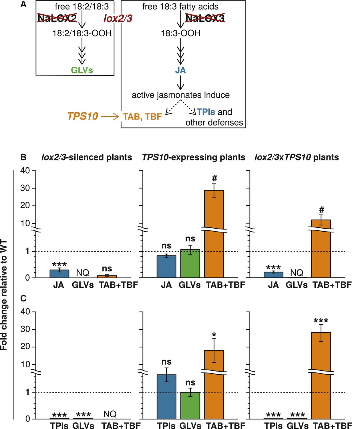
Transgenic lines manipulated in the emission of TAB, TBF, and GLVs, and the production of total jasmonate-mediated defenses (Figure 1 and associated source data files) were screened and characterized as described in Appendix 1. To investigate the community-level effects of variation in TAB and TBF in well- and poorly defended plants, we used four genotypes: WT plants, which have jasmonate-mediated induced direct defense compounds and herbivore-induced volatile emission comprising primarily sesquiterpenes and GLVs; TPS10 plants, which are like WT but have both enhanced induced, as well as constitutive emission of the herbivore-induced sesquiterpenes TAB and TBF (Schuman et al., 2014); lox2/3 plants, which are deficient in both jasmonate-mediated direct defense compounds and herbivore-induced volatiles, and lox2/3xTPS10 plants, which are like lox2/3, but with constitutive emission of TAB and TBF.
Figure 1
The lox2/3 and TPS10 transgenic constructs, alone and in combination (lox2/3xTPS10), independently alter herbivore-induced plant defenses and sesquiterpene HIPVs.
(A) The endogenous lipoxygenase genes LOX2 and LOX3 and the Z. mays sesquiterpene synthase gene TPS10 (TPS10) were manipulated in transgenic lines of N. attenuata in order to uncouple the production of two HIPVs—the sesquiterpenes (E)-α-bergamotene (TAB) and (E)-β-farnesene (TBF)—from jasmonate-mediated direct defenses and other volatiles. LOX2 and LOX3 provide fatty acid hydroperoxides from 18:2 and 18:3 fatty acids (18:2/18:3-OOH) for the synthesis of green leaf volatiles (GLVs) or jasmonic acid (JA) and the jasmonate-derived hormones, respectively. GLVs are released in response to herbivore damage, and jasmonates regulate the production of most anti-herbivore defenses, including trypsin protease inhibitors (TPIs), and other HIPVs. LOX2 and LOX3 were transgenically silenced using an inverted repeat (ir) construct specifically silencing both (lox2/3). Jasmonate-regulated volatiles in N. attenuata are mostly sesquiterpenes, of which the most prevalent is TAB, and include trace amounts of the biosynthetically related sesquiterpene TBF. The Z. mays sesquiterpene synthase TPS10 (Köllner et al., 2009), which produces TAB and TBF as its main products, was ectopically over-expressed in N. attenuata plants under control of a 35S promoter (TPS10) to uncouple the emission of these volatiles from endogenous jasmonate signaling. (B and C) Plants with lox2/3 and TPS10 constructs, and a cross with both constructs having the transgenes in a hemizygous state (lox2/3xTPS10) had the expected phenotypes both in glasshouse and field experiments. For each compound or group of compounds, the mean WT value was set to 1 (indicated by dashed lines), and all values were divided by the WT mean resulting in mean fold changes ±SEM. A complete description of TPS10 plants including the demonstration of a single transgene insertion and WT levels of non-target metabolites is provided in Schuman et al. (2014), and additional information for lox2/3, TPS10, and lox2/3xTPS10 plants (single transgene insertion for lox2/3, accumulation of target gene transcripts) is given in Appendix 1. (B) Glasshouse-grown plants were treated with wounding and M. sexta OS, and JA, GLVs, TAB and TBF were analyzed at the time of peak accumulation; n = 4. For lox2/3 and lox2/3xTPS10, GLVs were not quantifiable (NQ) by GC–MS due to inconsistently detected or no detected signals. ***p<0.001 in Tukey HSD tests following a significant one-way ANOVA (p<0.001) of WT, lox2/3, and lox2/3xTPS10; # plants with the TPS10 construct emit significantly more TAB + TBF (Holm-Bonferroni-corrected p<0.01 in a Wilcoxon rank sum test of WT and lox2/3 vs lox2/3xTPS10 and TPS10); ns, not significant. TBF was not detectable in lox2/3 or WT samples. For absolute amounts of JA and other phytohormones, GLVs, TAB and TBF measured in glasshouse samples, see Figure 1—source data 1, 2. (C) TPI activity, total detectable GLVs, and total TAB and TBF measured in frozen leaf samples harvested from field-grown plants at the end of experimental season two (June 28th), after plants had accumulated damage from naturally occurring herbivores. TPIs (n = 11–24) were slightly elevated in field samples of TPS10 plants, but TPI activity did not differ from WT plants in glasshouse samples from two independent TPS10 lines including the line used for this study (Schuman et al., 2014). Total GLVs, TAB, and TBF were quantified by GC–MS in hexane extracts from the same tissue samples used to measure TPI activity, n = 9–22 (a few samples had insufficient tissue for the analysis). Neither TAB nor TBF could be detected in lox2/3 samples (NQ); TBF was also not detectable in WT samples. *Corrected p<0.05, ***corrected p<0.001 in pairwise Wilcoxon rank sum tests following significant (corrected p<0.05) Kruskal–Wallis tests across all genotypes for each category; p-values were corrected for multiple testing using the Holm-Bonferroni method; ns, not significant. For absolute amounts of TPIs, GLVs, TAB and TBF, and non-target volatiles measured in field-collected tissue samples, see Figure 1—source data 3; emission of GLVs, TAB, TBF, and non-target volatiles from field-grown plants is given in Appendix 2.
-
Figure 1—source data 1
Absolute values for JA and GLVs shown as fold-changes in Figure 1B in lox2/3 and lox2/3xTPS10 plants, as well as JA-Ile, individual GLVs, and leaf areas for headspace collection (mean ± SEM); n = 4.
Data are from a single glasshouse experiment. Values for TPS10 (line 10–3) are reported in Schuman et al. (2014).
- https://doi.org/10.7554/eLife.04490.004
-
Figure 1—source data 2
Absolute values for TAB and TBF shown as fold-changes in Figure 1B, and leaf areas for headspace collection (mean ± SEM); n = 4.
Data are from a single glasshouse experiment.
- https://doi.org/10.7554/eLife.04490.005
-
Figure 1—source data 3
Absolute values for analytes shown as fold-changes in Figure 1C (mean ± SEM).
Data are from tissue samples of several pooled leaves per plant from field-grown plants, taken at the end of experimental season two (June 28th).
- https://doi.org/10.7554/eLife.04490.006
These genotypes were grown as individuals and in five-plant populations in a field plot in N. attenuata's native habitat (Figure 2A, Figure 2—figure supplements 1, 2). A population size of five plants is realistic for natural populations of N. attenuata (Figure 2—figure supplement 3), particularly before 1995, after which an invasive brome grass fueled a dramatic increase in fire sizes and consequently N. attenuata population sizes. This choice of population size also allowed us to clearly differentiate between edge and center positions (Figure 2B). Populations were either monocultures, or mixed cultures containing a single TPS10-expressing plant at the center and plants of the same defense- and HIPV level at the edges (WT around TPS10, and lox2/3 around lox2/3xTPS10, Figure 2B).
Figure 2 with 3 supplements see all
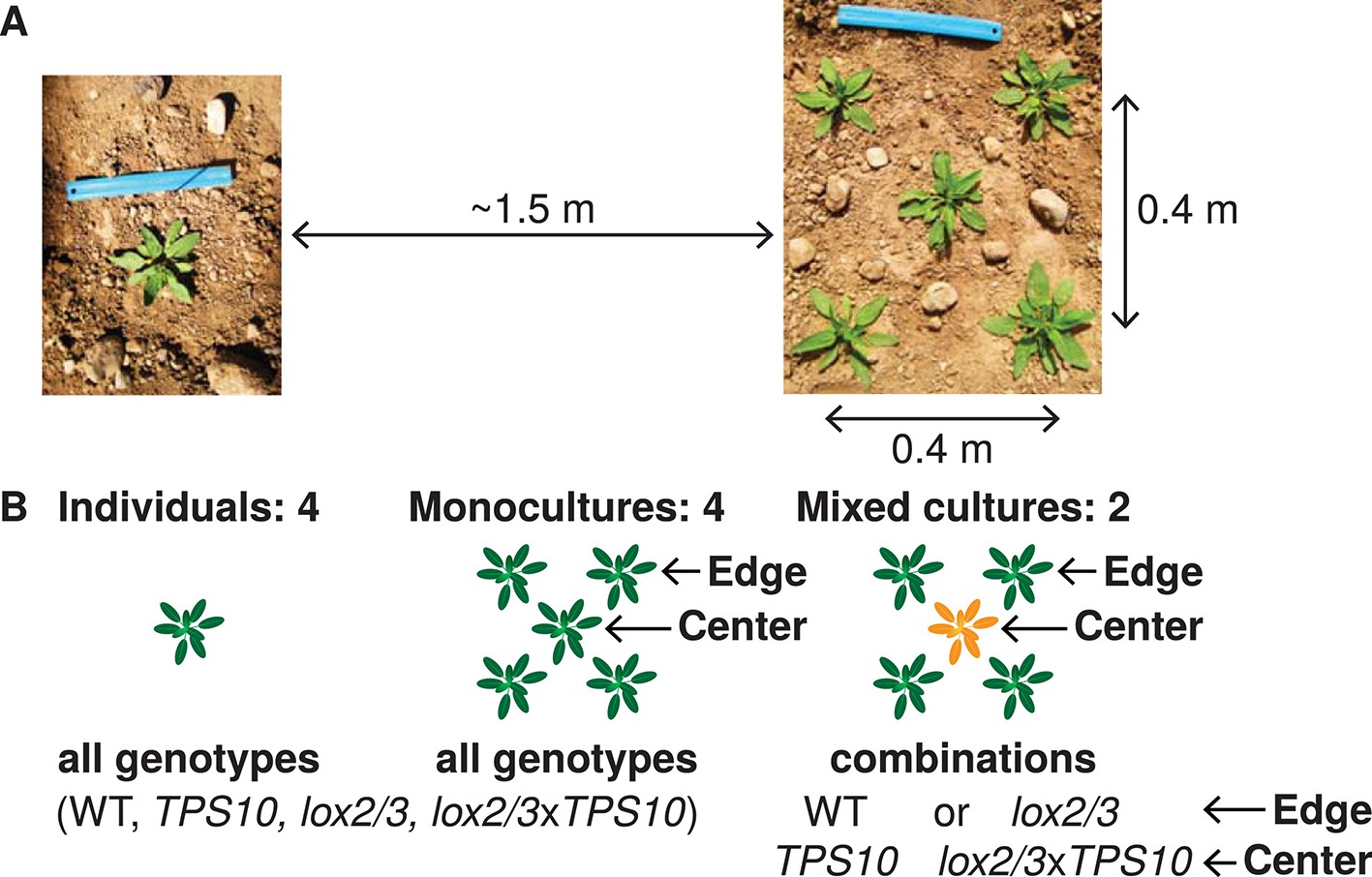
Field experiments designed to measure genotype-by-population effects of TPS10 volatiles in well-defended (WT, TPS10) or poorly defended (lox2/3, lox2/3xTPS10) plants.
Two similar experiments were conducted in two consecutive field seasons. (A) Each genotype was planted as individuals and in five-plant populations (see Figure 2—figure supplement 1). Each individual or population was planted ca. 1.5 m from the nearest neighboring individual/population, measured perimeter-to-perimeter. Populations consisted of five plants arranged as shown in a 0.4 × 0.4 m square. (B) Individual and population types: monocultures and, additionally, mixed cultures were planted in which a TPS10 plant (TPS10 or lox2/3xTPS10) was surrounded by four plants of the same level of jasmonate-mediated defense and GLVs (WT or lox2/3). Replicates (n = 12 in season one, 15 in season two of each individual or population type) were arranged in a blocked design (see Figure 2—figure supplement 2): blocks consisting of one replicate of each type (all six randomly-ordered populations followed by all four randomly-ordered individuals) were staggered such that consecutive blocks were not aligned, and thus populations and individuals were also interspersed. Random order was modified only when necessary to ensure that no two replicate individuals/populations were placed next to each other vertically, horizontally, or diagonally. This planting design reflects typical distributions in native populations of Nicotiana attenuata (see Figure 2—figure supplement 3), particularly before 1995, after which an invasive brome grass fueled a dramatic increase in fire sizes and consequently N. attenuata population sizes.
There was no effect of population type (individual, monoculture, mixed culture) or plant position (individual, edge, center) on genetically engineered levels of GLVs, jasmonate-mediated defense (trypsin protease inhibitor [TPI] activity served as an indicator), TAB and TBF (Figure 1C, Figure 1—source data 3 and details in Appendix 2), with one exception: trace amounts of TAB were detected in open headspace trappings around young lox2/3 plants at the edges of lox2/3 + lox2/3xTPS10 mixed cultures, but not around lox2/3 individuals or lox2/3 plants at the edges of monocultures (Figure 3).
Figure 3

The TPS10 product TAB can be detected in the open headspace around lox2/3 plants in mixed cultures containing a lox2/3xTPS10 plant.
(A) An ‘open headspace’ trapping was conducted during season two (May 16th) with rosette-stage individuals and edge plants as shown, using activated charcoal filters shielded from ozone and UV by MnO2-coated copper ozone scrubbers (black strips in Teflon tubes pointed at plant) and aluminum foil, respectively. The headspace was sampled during the day, when sesquiterpenes are most abundant (see Appendix 2). Eluents from all four filters were combined and analyzed using highly sensitive GCxGC-ToF analysis; n = 4 plants. (B) The TPS10 product trans-α-bergamotene (TAB) could be detected in the open headspace of two of four lox2/3 plants at the edges of mixed cultures containing a lox2/3xTPS10 plant, but not in lox2/3 individuals or lox2/3 plants in monocultures. Peak areas were normalized to the internal standard (IS) peak. Arrows indicate the plant that was sampled.
LOX2 and LOX3 expression reduce foliar herbivore abundance and damage, while TPS10 expression further reduces herbivore abundance
Prior to the field experiment, we tested whether TPS10 expression affects defense against a specialist herbivore in a WT or LOX2/3-deficient background via a no-choice assay with larvae of the naturally co-occurring solanaceous specialist Manduca sexta in the glasshouse. M. sexta larvae grew five times as large on lox2/3 or lox2/3xTPS10 plants as they did on WT or TPS10 plants (Figure 4; Wilcoxon rank sum tests, Holm-Bonferroni-corrected p-values <0.001). In contrast, larvae grew to similar sizes on plants that differed only in the TPS10 overexpression construct (corrected p-values >0.2). The progression of M. sexta larval instars was also faster on LOX2/3-deficient plants: all larvae feeding on lox2/3 or lox2/3xTPS10 were in the third instar by day 8, while 11/17 larvae feeding on WT and 12/15 larvae feeding on TPS10 were still in the second instar (corrected p<0.001 in Fisher's tests for lox2/3 v. WT, lox2/3 v. TPS10, lox2/3xTPS10 v. WT, and lox2/3xTPS10 v. TPS10, corrected p=0.4440 for WT v. TPS10, and corrected p=1 for lox2/3 v. lox2/3xTPS10).
Figure 4
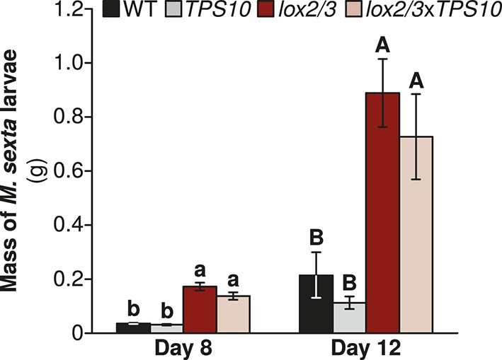
Manduca sexta larvae grow larger on LOX2/3-deficient plants, regardless of TPS10 expression, in a glasshouse experiment.
Data are shown as mean ± SEM; n = 15–19 larvae on day 8 and 11–16 larvae on day 12. One M. sexta neonate per plant (starting n = 25 larvae) was placed immediately after hatching on the youngest rosette leaf of an elongated plant. Larvae were weighed at the third and fourth instars (of 5 total), corresponding to days 8 and 12, after which larvae become mobile between plants. a,b/A,B Different letters indicate significant differences (corrected p<0.001) in larval mass on different plant genotypes within each day, in Wilcoxon rank sum tests following significant (corrected p<0.001) Kruskal–Wallis tests for each day (WT vs lox2/3 day 8, W17,19 = 310, corrected p<0.001, day 12, W15,15 = 217, corrected p<0.001; TPS10 vs lox2/3xTPS10, day 8, W15,20 = 290, corrected p<0.001, day 12, W11,14 = 143, corrected p<0.001; WT vs TPS10 day 8, W17,15 = 95, corrected p=0.227, day 12, W15,11 = 56, corrected p=0.361; lox2/3 vs lox2/3xTPS10 day 8, W19,20 = 249, corrected p=0.201, day 12, W16,14 = 134, corrected p=0.377). p-values were corrected for multiple testing using the Holm-Bonferroni method.
In the field, total canopy damage from foliar herbivores was assessed on June 9th in season one, and June 2nd in season two. Canopy damage in both seasons was due to both generalist and specialist herbivores from chewing and piercing-sucking feeding guilds. The generalists included noctuid larvae, Trimerotropis spp. grasshoppers, Oecanthus spp. tree crickets, and leaf miner spp.; the specialists included the sphingid larvae M. sexta and Manduca quinquemaculata, flea beetles Epitrix hirtipennis and E. subcrintia, and the mirid Tupiocoris notatus. Canopy damage from herbivores was more than twice as great in season two (9–24% total canopy) as in season one (2–9% total canopy).
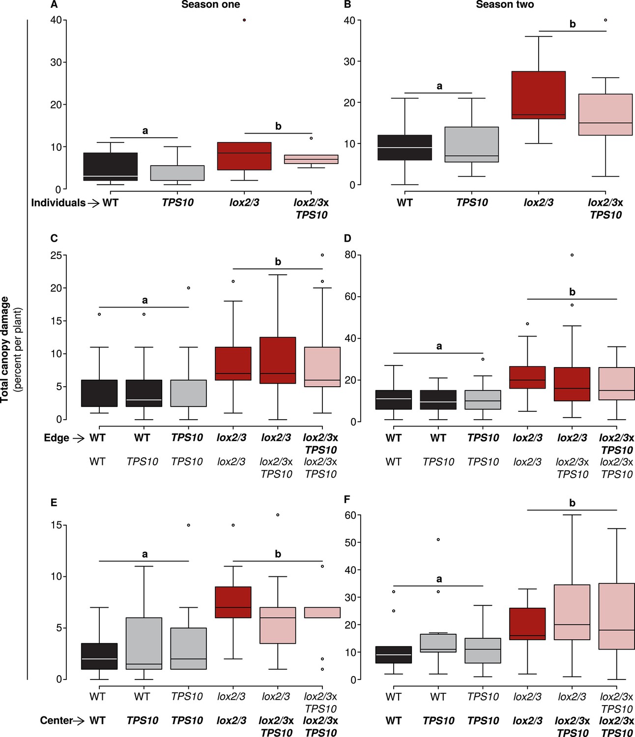
In both seasons, lox2/3 and lox2/3xTPS10 plants accumulated twice as much canopy damage as WT and TPS10 plants, regardless of plant position or population type (Figure 5 and associated source data files): there were no significant differences during either season between plants or populations differing only in TPS10 expression, or plants of the same genotype in mono- vs mixed cultures with single TPS10-expressing plants; details of statistical tests are given in Appendix 3.
Figure 5
Only LOX2/3 and not TPS10, plant position, or population type determined total foliar damage from herbivores over two consecutive field seasons.
Note differences in y-axis scale. Data were collected on June 9th in season one (left panels), and on June 2nd in season two (right panels) from plants at all different positions in the experiment: individual plants (A–B), and plants at the edges (C–D) or at the centers (E–F) of populations. Black bars denote WT, grey bars TPS10, red bars lox2/3, and pink bars lox2/3xTPS10 plants. Total canopy damage reflected the trends in canopy damage caused by individual herbivores (Figure 5—source data 1, 2). Total canopy damage in season one was low (left panels), ranging from 5–10% on lox2/3 and lox2/3xTPS10 plants, and only 2–5% on WT and TPS10 plants. Damage levels were about twice as high in season two (right panels), but showed the same relative pattern, with LOX2/3-deficient plans having more damage. Damage levels within a season were similar for plants in different positions (p>0.07, see Appendix 3). a,b Different letters indicate significant differences (p<0.05) between LOX2/3-expressing and LOX2/3-deficient plants (WT, TPS10 v. lox2/3, lox2/3xTPS10) in minimal ANOVA or linear mixed-effects models on arcsin-transformed data. For individuals and center plants n = 7–13, and for edge plants n = 16–48 (up to 4 per population; the blocking effect was accounted for by a random factor in statistical analysis); exact replicate numbers are given in Figure 5—source data 1, 2. There were no significant differences in damage between plants differing only in TPS10 expression (p>0.4), plants in mono- vs mixed cultures (p>0.5), or plants of the same genotype at different positions (individual, edge, or center, p>0.07). Statistical models are given in Appendix 3.
-
Figure 5—source data 1
Total canopy damage from individual herbivores or groups of herbivores in experimental season one, corresponding to data shown in Figure 5A (mean ± SEM).
- https://doi.org/10.7554/eLife.04490.014
-
Figure 5—source data 2
Total canopy damage from individual herbivores or groups of herbivores in experimental season two, corresponding to data shown in Figure 5B (mean ± SEM).
- https://doi.org/10.7554/eLife.04490.015
Damage observed could be attributed to specific herbivores according to typical feeding patterns and the observation of feeding individuals. Individual herbivores generally followed the trend of total herbivore damage, causing greater damage on lox2/3 and lox2/3xTPS10 plants (Figure 5—source data 1, 2). The largest and most significant differences (p-values < 0.05) were between plants with vs without the lox2/3 silencing construct (lox2/3 and lox2/3xTPS10 v. WT and TPS10, statistical comparisons in Figure 5—source data 1, 2). All significant differences were between plants or populations with vs without the lox2/3 silencing construct, and never between plants or populations differing only in the TPS10 overexpression construct, nor between plants of the same genotype in different population types (Figure 5 and associated source data files). It should be noted that in season one, multiple lepidopteran species were present on plants and their damage could not be clearly distinguished; since these included generalist species as well as Manduca spp., lepidopteran damage in season one also could not be categorized as generalist or specialist damage (Figure 5—source data 1). In season two, lepidopteran damage not resulting from experimental infestation for predation assays (not counted toward total canopy damage) was due to noctuid species (Figure 5—source data 2).
The abundance of arthropods on plant shoots was quantified for a subset of plants on June 26th in season two, at which time T. notatus adults and nymphs and Epitrix spp. adults were the only foliar herbivores observed. Interestingly, total herbivore abundance at the end of the season did not entirely reflect foliar herbivore damage assessed on June 9th (Figure 5B), although a visual assessment of the plants indicated that relative herbivore damage levels still reflected the June 9th data: herbivores were less abundant on plants expressing TPS10, independently of lox2/3 expression (Figure 6A and associated source data files). Herbivore abundance on WT plants differed depending on plants' location: in a comparison of abundance on individuals vs plants at the edges or centers of monocultures, abundance was highest on individuals and lowest on center plants. In contrast, herbivore abundance on TPS10-expressing plants did not depend on plant location (Figure 6B, Appendix 3). Foliar herbivore abundance on WT and lox2/3 edge plants was not affected by the presence of a TPS10-expressing neighbor: neither population type (monoculture or mixed culture), nor the interaction of genotype with population type was significant. However for WT and lox2/3 edge plants, herbivore abundance did vary as a function of genotype, with abundance indeed being greater on lox2/3 edge plants (Figure 6C, Appendix 3), consistent with greater damage to these plants (Figure 5D).
Figure 6
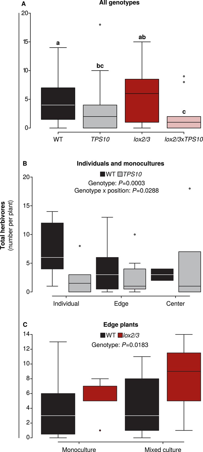
Foliar herbivore abundance is determined by TPS10 expression, lox2/3 expression, and plant position.
Data were collected on June 26th in season two, when herbivores and predators were more abundant (see Figure 5). Black denotes WT, grey TPS10, red lox2/3, and pink lox2/3xTPS10 plants. Counts for individual herbivores and predators are given in Figure 6—source data 1, 2. (A) Herbivore counts on focal plants of each genotype revealed fewer herbivores present on plants expressing TPS10 (n given in Figure 6—source data 1). a,b Different letters indicate significant differences (corrected p<0.05) between genotypes in Tukey contrasts following significant differences in a generalized linear mixed-effects model (see Appendix 3). (B) For WT and TPS10 individuals or plants in monocultures (n given in Figure 6—source data 2), there was a significant effect (p<0.05) of plant genotype (z = −3.662, p=0.0003) and an interaction of genotype with position (TPS10 by center vs individual position, z = 2.186, p=0.0288, generalized linear mixed-effects model in Appendix 3). (C) The presence of a TPS10-expressing neighbor in mixed populations did not significantly affect herbivore abundance on WT or lox2/3 edge plants, but there was a significant difference between WT and lox2/3 genotypes at the edges of populations (n given in Figure 6—source data 2, z = 2.358, p=0.0183, generalized linear model in Appendix 3).
-
Figure 6—source data 2
Total and median numbers of herbivores counted on focal plants of different genotypes on June 26th in season two, broken down into different population types and plant locations for WT and TPS10 plants.
Replicate numbers of lox2/3 and lox2/3xTPS10 plants were not sufficient for this analysis (n ≤ 3 per population type and position).
- https://doi.org/10.7554/eLife.04490.017
-
Figure 6—source data 1
Total and median numbers of herbivores and predators counted on focal plants of different genotypes on June 26th in season two.
- https://doi.org/10.7554/eLife.04490.018
Thus LOX2 and LOX3 expression increased plants' susceptibility to foliar herbivores, measured as herbivore growth or percentage of plant canopy damaged (Figures 4, 5), but the relationship between foliar herbivore abundance and LOX2/LOX3 expression was more complex and dependent on plants' position in populations (Figure 6). In contrast, herbivore abundance, but not damage or performance, was consistently reduced on TPS10-expressing plants (Figures 4–6).
LOX2/3 deficiency accelerates flowering under low herbivory, while TPS10 expression reduces flower production under high herbivory
We monitored plant growth and size, to control for these non-defense traits which could confound the analysis of differences among genotypes, plant positions, and population types, and their interactions with insect communities. Rosette diameter and plant stem height were measured at three times during the main period of vegetative growth in season one (May 1st–2nd, 8th–11th, and 16th–17th), and after plants had transitioned from vegetative growth to reproduction in season two (June 4th–6th), at which time stem diameter was also measured. There were no significant differences in rosette diameter or stem diameter (p-values >0.08 in ANOVAs or linear mixed-effects models with LOX2/3 deficiency and TPS10 expression, plant position, and population type as factors: see statistical approach in Appendix 3). There were few differences in final measurements of plant height. LOX2/3-deficient plants were slightly taller at the final size measurement on May 17th of season one: the stem height of WT plants was 28.5 ± 1.1 cm, TPS10 plants 27.2 ± 1.5 cm, lox2/3 plants 35.4 ± 1.2 cm, and lox2/3xTPS10 plants 32.2 ± 1.5 cm (mean ± SEM). In season two, final measurements of plant height on June 6th revealed only a minor difference for central plants expressing TPS10, discussed below. Statistical analyses of plant height are given in Figure 8—source data 1.
We also monitored early flower production by plants as a measure of growth and reproduction rates. To assess the rate of flowering, flowers were counted once shortly after plants first began to flower, and again 1 week later; in season two, plant size and flower production was additionally assessed once immediately prior to quantification of herbivore damage. In season one, in which herbivores damaged <10% of total canopy area (Figure 5), LOX2/3-deficient plants produced more flowers earlier than WT and TPS10 plants. Shortly after the first plants began to flower in season one (May 11th), more lox2/3 and lox2/3xTPS10 than WT and TPS10 plants were flowering (30% v. 14%), and this was still true 1 week later, after most plants had flowers (95% v. 79%; G-tests of independence, corrected p<0.001 on May 11th and 17th; Figure 7A). In pairwise comparisons among individual genotypes, there were no significant differences in G-tests of independence between WT and TPS10 (corrected p-values > 0.2) or lox2/3 and lox2/3xTPS10 (corrected p-values >0.7). However, more lox2/3 than WT plants were flowering at both timepoints (May 11th corrected p<0.001, May 17th corrected p=0.022), and more lox2/3xTPS10 than TPS10 plants were flowering on May 17th (corrected p<0.001). Both lox2/3 and lox2/3xTPS10 plants also produced more flowers per plant: on May 17th lox2/3 had 6 (median = mean) flowers per plant while WT had 4, and lox2/3xTPS10 had 4/5 (median/mean) flowers per plant while TPS10 had 2/3.
Figure 7
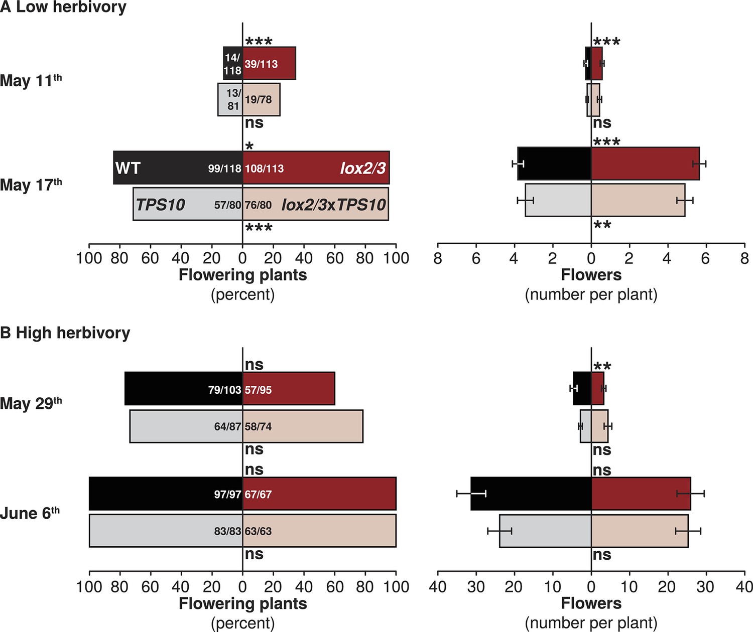
LOX2/3 deficiency accelerated flowering under low herbivory.
Flower production was monitored twice per season: once shortly after plants began to flower and again 1 week later, when most or all plants were flowering. Bars indicate either total percentage of plants of each genotype which were flowering (left panels), or the mean number of flowers per plant (right panels). WT and TPS10 (black and grey bars) are shown opposite lox2/3 and lox2/3xTPS10 (red and pink bars). Ratios in bars indicate numbers of flowering/total plants monitored; a few plants were not included in counts which had recently lost their main stem to herbivores and had not yet re-grown. (A) In season one, when plants suffered less damage from herbivores (Figure 5), plants with the lox2/3 silencing construct produced more flowers earlier: asterisks indicate pairwise differences between genotypes differing only in the lox2/3 silencing construct. ***Corrected p<0.001, **corrected p<0.01, *corrected p<0.05, or no significant difference (ns) in G-tests (percentage flowering) or in Wilcoxon rank sum tests (flower number, WT vs lox2/3: May 11th, W120,120 = 8582, p=0.0002; May 17th, W120,119 = 5043, p<0.0001; TPS10 vs lox2/3xTPS10: May 11th, W84,84 = 3801, p=0.2063; May 17th, W84,84 = 2520, p=0.0027). (B) In season two, during which plants received more damage from herbivores (Figure 5), flowering was monitored at later dates: the first timepoint in (B) is comparable to the second timepoint in (A) in terms of the proportion of plants flowering and the average number of flowers per plant (note difference in scale). In season two, LOX2/3 deficiency rather decreased early flower numbers in the comparison of WT vs lox2/3 on May 29th, and did not increase flower numbers at either measurement (WT vs lox2/3: May 29th, W103,95 = 3860.5, p=0.0091; June 6th, W97,69 = 2940.5, p=0.3018; TPS10 vs lox2/3xTPS10: May 29th, W87,74 = 3646.5, p=0.1417; June 6th, W83,63 = 2695, p=0.7518). For a complete analysis of the effects of LOX2/3 deficiency and TPS10 expression, plant position, and population type on flowering and plant size, see source data file for Figure 8.
In season two, when herbivore damage ranged from 10–24% of total canopy (Figure 5), LOX2/3-deficient plants did not flower earlier (Figure 7B). Plants were in an earlier stage of flowering on May 29th in season two, than on May 17th in season one: both the proportion of flowering plants (72% May 29th season two, 87% May 17th season one) and the mean number of flowers per plant (4 on May 29th season two, 5 on May 17th season one) were lower for the May 29th observation. The differences between plants with or without the lox2/3 silencing construct, which was evident on May 17th in season one, were not observed on May 29th in season two: the proportion of flowering plants was similar for all genotypes (68% for lox2/3 and lox2/3xTPS10 v. 75% for WT and TPS10, G-test of independence, corrected p = 1), as was the average number of flowers per plant: 1/3 (median/mean) for lox2/3, 3/5 for WT, 2/4 for lox2/3xTPS10, and 2/3 for TPS10. 1 week later, 100% of plants were flowering, and the median number of flowers per plant remained similar regardless of LOX2/3 deficiency (Figure 7B).
However, in season two, there were subtler effects on flower production which could be attributed to plant position, LOX2/3 deficiency, and TPS10 expression (Figure 8). The plant height and flowering data collected immediately prior to the assessment of herbivore damage in season two were analyzed as described in Appendix 3 for effects of LOX2/3 deficiency, TPS10 expression, plant position, and population type (statistical analysis in the source data file for Figure 8). There were almost no differences in plant height (Figure 8, left panels), indicating that plant size differed little; the only significant difference was a small negative effect of TPS10 expression for plants in the centers of populations, most pronounced in mixed cultures (Figure 8E). In contrast, flower production of individual plants was strongly decreased by TPS10 expression and only slightly decreased by LOX2/3 deficiency (Figure 8B), but differed little for plants in populations (Figure 8, right panels), with the exception that the shorter central plants also produced slightly fewer flowers (Figure 8F). Interestingly, for individual plants, there was an interactive effect of TPS10 expression and LOX2/3 deficiency resulting in similar flower production for lox2/3xTPS10 plants and WT plants, although both lox2/3 individuals and TPS10 individuals produced significantly fewer flowers than WT (Figure 8B, statistical analysis in the source data file for Figure 8).
Figure 8
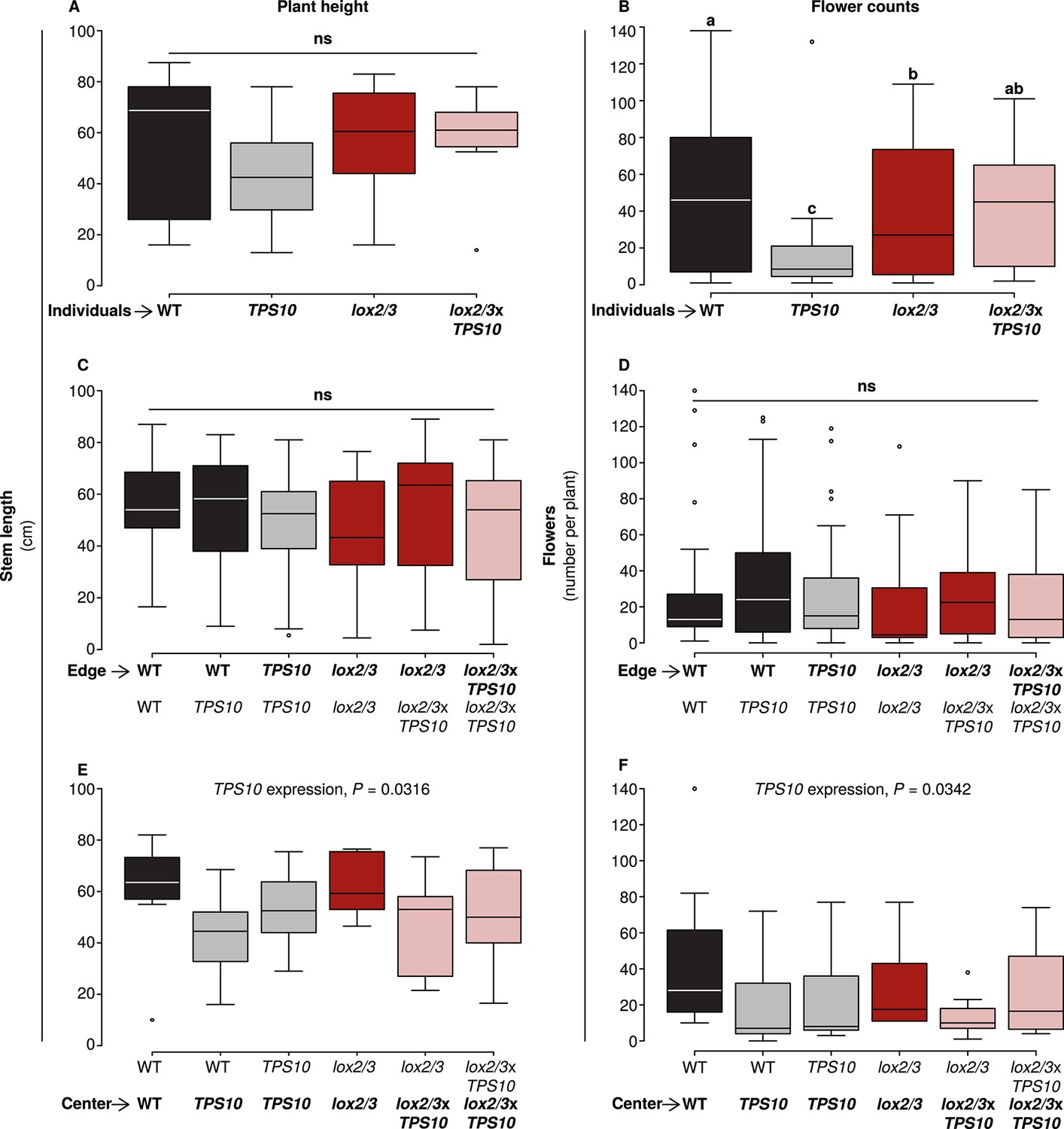
TPS10 expression reduced flower production under high herbivory.
Plant size as measured by stem length (left panels), and reproduction as measured by flower production (right panels); n given in Figure 8—source data 1. Data were collected on June 6th in season two from plants at all different positions in the experiment: individual plants (A–B), and plants at the edges (C–D) or at the centers (E–F) of populations. Black bars denote WT, grey bars TPS10, red bars lox2/3, and pink bars lox2/3xTPS10 plants. Plant height differed little, with only a small negative effect of TPS10 expression for center plants (E), which was more pronounced in mixed- than monocultures, indicating a slight competitive disadvantage for these plants. Individual plants differed much more than plants in populations in terms of flower production, with TPS10-expressing plants at a disadvantage (B); this effect was greatly reduced in populations.a,b Different letters indicate significant differences (corrected p<0.05) in Tukey post-hoc tests on plant genotype following significant effects in a generalized linear model, or generalized linear mixed-effects model (C–D) with genotype as a factor; these p-values were corrected using the Holm-Bonferroni correction for multiple testing as the same data were also tested for effects of LOX2/3 deficiency and TPS10 expression (see Figure 8—source data 1). There was no difference in flower production for edge plants, but a small negative effect of TPS10 expression on flower production in center plants (F) corresponding to the slight reduction in height of these plants (E). Statistical models are given in Figure 8—source data 1.
-
Figure 8—source data 1
The same statistical approach described in Appendix 3 for Figure 5 was used for plant size and reproduction data from May 17th in season 1, and June 6th in season two (the most complete measurements, closest to the date of herbivore damage screens, from each season).
It should be kept in mind that plants in the season one analysis were at an earlier stage of growth and flowering, for example, had about 10% as many flowers as plants in the season 2 analysis; for an analysis of flowering at similar stages, see Figure 7. Significant p-values and factors are given in bold, while p-values and factors marked in grey and in bold are marginal, but are required in the minimal model because their removal resulted in poorer (higher) AIC values. Other non-significant factors remained in models because they were the least insignificant factor (if only one factor remained), or because they are dependent on other factors which are significant or required.
- https://doi.org/10.7554/eLife.04490.021
Overall, these data indicate that accelerated reproduction of LOX2/3-deficient plants in season one was due to a reduced net cost for these plants of LOX2/3-mediated defenses under low herbivore damage, which disappeared under higher herbivore damage in season two (Figures 7, 8 and associated source data file). In contrast, TPS10 expression had little effect on plant growth and flowering in season one (Figure 7, source data file for Figure 8) and the effects of TPS10 expression on flowering in season two depended strongly on plant position (individual, edge or center, Figure 8 and associated source data file). This indicates that TPS10 expression did not have large, direct costs for plants in the field, but that the reproductive output of TPS10 plants was sensitive to the presence and identity of neighbor plants. Especially under high herbivory in season two, there were few differences in plant size and these did not correspond to differences in herbivore damage (Figures 5, 8).
LOX2/3 deficiency increases plant mortality, but mortality is mitigated by single TPS10-expressing plants in LOX2/3-deficient populations
We quantified plant mortality as an unambiguous measure of plant health and fitness (Figure 9). In our experiments, mortality can be interpreted as a measure of total reproductive potential and thus Darwinian fitness, because we observed mortality of plants before, or during, the peak of their flower production, and ended our experiments when plants would normally produce mature seed. (Production of viable seed is not generally allowed for field-released transgenic plants, and we did not allow our plants to produce seed.)
Figure 9 with 1 supplement see all
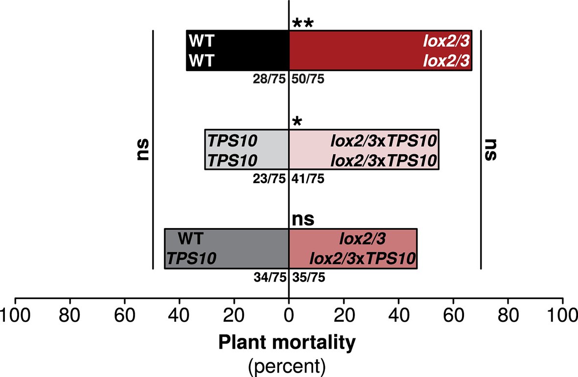
One TPS10-expressing plant per population counteracts a mortality increase in LOX2/3-deficient populations.
Bars indicate total percentage mortality for all plants in each population type, and ratios in bars indicate numbers of dead/total plants (n = 75). WT and TPS10 populations (left, black, and grey bars) are compared to the equivalent lox2/3 and lox2/3xTPS10 populations (right, red, and pink bars) differing only in the lox2/3 silencing construct. LOX2/3-deficient plants had higher mortality in monocultures, regardless of whether they also expressed TPS10 (**WT mono v. lox2/3 mono, corrected p<0.01; *TPS10 mono v. lox2/3xTPS10 mono, corrected p<0.05 in G-tests; p-values were corrected for multiple testing using the Holm-Bonferroni method). However, the mortality of plants in mixed lox2/3 + lox2/3xTPS10 populations is similar to that of the plants in mixed WT + TPS10 populations (ns, not significant). There was no significant difference in mortality among mono- and mixed cultures of WT and TPS10 plants (corrected p>0.3), or of lox2/3 and lox2/3xTPS10 plants, although there was a marginal difference between lox2/3 monocultures and lox2/3 + lox2/3xTPS10 mixed cultures (corrected p=0.091). In addition, a health index was assigned to each plant (discussed in text); this index was correlated with several plant growth and reproduction parameters (see Figure 9—figure supplement 1). Data were collected on June 29th at the end of experimental season two; in season one, all plants experienced much lower herbivory (Figure 5) and negligible mortality (0–5%).
In season one, mean plant mortality was only 1%, or a total of 6 plants, by the end of experiments in mid-June. However, in season two, greater damage from herbivores (Figure 5) was associated with much higher mean plant mortality: 46%, or 236 plants by the end of experiments on June 29th. Overall, LOX2/3-deficient plants had higher mortality: 55% for lox2/3 and lox2/3xTPS10 vs 38% for WT and TPS10 plants (G-test of independence, corrected p = 0.002). Thus, lox2/3 plants in monocultures had significantly higher mortality than WT plants in monocultures (corrected p=0.003), and lox2/3xTPS10 plants in monocultures had significantly higher mortality than TPS10 plants in monocultures (corrected p=0.022) (Figure 9). In contrast, mortality rates for plants in mixed cultures were similar regardless of LOX2/3 deficiency (corrected p=0.870). This was associated with marginally decreased mortality for plants in lox2/3 + lox2/3xTPS10 mixed cultures (Figure 9, lox2/3 mono v. lox2/3 + lox2/3xTPS10 mix, corrected p=0.092). Interestingly, mortality in WT + TPS10 mixed cultures was slightly higher than in monocultures (45% v. 37% for WT monocultures and 31% for TPS monocultures), although these differences were also not significant (corrected p-values >0.090).
In summary, because plants in lox2/3xTPS10 monocultures had higher mortality than those in TPS10 monocultures, we conclude that expression of TPS10 by LOX2/3-deficient plants did not compensate for the absence of LOX2/3-mediated defenses; yet surprisingly, single lox2/3xTPS10 plants in lox2/3 + lox2/3xTPS10 mixed populations reduced the mortality of the entire population to the same level as in WT + TPS10 mixed populations.
LOX2/3-deficient plants have reduced apparent health, unless they have TPS10-expressing neighbors
Plant health, in terms of turgor, expanded leaf area and senescence, varied noticeably under the higher levels of herbivore damage in season two (Figure 5), and so plants were given an apparent health rating on a scale of one (dead) or two (low) to five (high). This scale was sufficiently objective that several observers were able to independently assign the same health index number to randomly-chosen plants, after training on fewer than 10 other plants. Ratings >1 on this health scale (living plants) were strongly correlated to several growth and reproduction traits measured (Spearman's ρ values ≥0.55, corrected p-values <0.001): number of buds, stem diameter, number of side branches, rosette diameter, stem length, and number of flowers (Figure 9—figure supplement 1).
LOX2/3 deficiency was associated with significantly poorer apparent health on this scale: excluding dead plants, a median health index of 3 for lox2/3 and lox2/3xTPS10 vs 3.5 for WT and TPS10 (Wilcoxon rank sum test, W153,186 = 19,057.5, corrected p<0.001). In pairwise tests between genotypes for surviving plants, WT appeared significantly healthier than lox2/3, but not lox2/3xTPS10 (WT v. lox2/3, W102,82 = 2722, corrected p<0.001; WT v. lox2/3xTPS10, W102,71 = 2687, corrected p=0.059); whereas TPS10 appeared significantly healthier than both lox2/3 and lox2/3xTPS10 (TPS10 v. lox2/3, W84,82 = 1996.5, corrected p<0.001; TPS10 v. lox2/3xTPS10, W84,71 = 1995, corrected p=0.006). There was no difference in the apparent health of WT vs TPS10 or lox2/3 vs lox2/3xTPS10 (corrected p-values=1, TPS10 v. WT, W84,102 = 4619; lox2/3 v. lox2/3xTPS10, W82,71 = 2604.5).
Separate examination of surviving individual, center, and edge plants revealed that LOX2/3 deficiency was only associated with poorer apparent health in edge plants (lox2/3 and lox2/3xTPS10 v. WT and TPS10: individuals, W21,22 = 230.5, corrected p=1; edge plants, W102,129 = 9544, corrected p<0.001; center plants, W30,35 = 598.5, corrected p=1). There were significant differences in the apparent health of edge plants in different population types: WT edge plants appeared significantly healthier than lox2/3 plants at the edges of monocultures, but not healthier than lox2/3 plants at the edges of lox2/3 + lox2/3xTPS10 mixed cultures (WT mono v. lox2/3 mono, W42,29 = 929, corrected p = 0.003; WT + TPS10 mix v. lox2/3 mono, W40,29 = 891.5, corrected p=0.003; WT mono v. lox2/3+lox2/3xTPS10 mix, W42,34 = 953, corrected p=0.164; WT + TPS10 mix v. lox2/3 + lox2/3xTPS10 mix, W40,34 = 892, corrected p=0.249). However, TPS10 plants at the edges of monocultures appeared significantly healthier than lox2/3 or lox2/3xTPS10 edge plants in mixed- or monocultures (TPS10 mono v. lox2/3 mono, W47,29 = 1129.5, corrected p<0.001; TPS10 mono v. lox2/3 + lox2/3xTPS10 mix, W47,34 = 1209.5, corrected p=0.001; TPS10 mono v. lox2/3xTPS10 mono, W47,39 = 1389.5, corrected p<0.001). No other comparisons between plants of individual population types were significant (corrected p-values >0.08) and there was no significant association between apparent health and plant position (Kruskal–Wallis test across individual, edge, and center plants, χ22 = 2.38, corrected p=1) or plants of the same genotype in mono- vs mixed cultures (Wilcoxon rank sum tests, corrected p-values=1).
In summary, as for foliar herbivore damage, growth, flowering, and mortality, there was no significant difference in the apparent health of plants differing only in TPS10 expression. However, TPS10 expression in lox2/3xTPS10 plants was associated with an apparent health similar to WT plants, while lox2/3 plants had a significantly lower apparent health than WT plants. Furthermore, the differences in apparent health were stronger between TPS10 plants and LOX2/3-deficient plants than between WT plants and LOX2/3-deficient plants, indicating a weak, positive effect of TPS10 expression on apparent plant health. Interestingly, lox2/3 plants at the edges of monocultures appeared less healthy than WT edge plants, but lox2/3 plants at the edges of lox2/3 + lox2/3xTPS10 mixed cultures did not, indicating a positive neighbor effect of TPS10 expression on the health of plants in LOX2/3-deficient populations.
TPS10-expressing plants increase the infestation rates of their neighbors by the stem-boring weevil Trichobaris mucorea
At the end of season two, we found that 35% of all surviving plants were infested with T. mucorea larvae. An adult T. mucorea is pictured in Figure 10A. Interestingly, TPS10 expression was associated with slightly higher infestation rates: 29% of lox2/3 and 34% of WT plants vs 39% of TPS10 and lox2/3xTPS10 plants. Looking at infestation rates by population type, we discovered a small difference between WT (34% infested) and TPS10 plants (39% infested) which masked a much larger effect: WT plants in WT + TPS10 mixed populations (55% infested) had an infestation rate more than twice that of WT plants in monocultures (19% infested, corrected p=0.015, Figure 10B). We observed the same tendency in lox2/3 and lox2/3xTPS10 populations: 33% of lox2/3 plants in mixed populations with lox2/3xTPS10 plants were infested, vs only 16% of lox2/3 plants in monocultures; interestingly, lox2/3xTPS10 plants tended to have higher infestation rates than lox2/3 plants in populations (Figure 10C). Likely due to higher plant mortality in lox2/3 populations (Figure 9), replicate numbers were too low for these effects to be significant (corrected p-values =1 for the comparison of infestation rates of lox2/3 plants in mono- vs mixed culture, and of lox2/3 vs lox2/3xTPS10 monocultures). Likely also due to low replicate numbers (n = 7–10), there were no significant differences in infestation among individuals (corrected p-values = 1 in pairwise tests), but 30% of TPS10, 38% of WT, 50% of lox2/3, and 57% of lox2/3xTPS10 individuals were infested. Based on these trends, had there been a significant effect for individuals, it would have been due to LOX2/3 deficiency and not TPS10 expression.
Figure 10
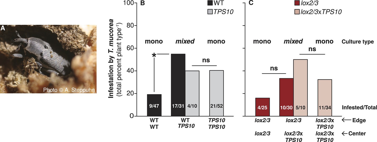
TPS10 plants increase the infestation rates of their WT neighbors with the stem-boring weevil T. mucorea.
(A) Photograph of a T. mucorea adult emerging from the stem which it infested as a larva reprinted with permission from Anke Steppuhn, Copyright 2005. All rights reserved. Adults mate and oviposit on young N. attenuata plants in March and April, and upon hatching, larvae burrow into the growing stem of the plant chosen by their mother (Diezel et al., 2011). Infestation was scored as the number of plants with hollow, frass-filled stems (from which larvae were usually also recovered). (B) T. mucorea infestation more than doubled for WT plants, but did not change for TPS10 plants in mixed cultures vs monocultures. Bars indicate total percentage of plants infested; ratios in bars indicate numbers of infested/total plants. Data were collected at the end of experimental season two (June 29th). *Corrected p<0.05 in a Fisher's exact test, n = 31–47 (all surviving replicates). p-values were corrected for multiple testing using the Holm-Bonferroni method. (C) The presence of lox2/3xTPS10 plants also tended to increase T. mucorea infestation in lox2/3 + lox2/3xTPS10 populations but, likely due to lower replicate numbers caused by higher mortality for plants in lox2/3 and lox2/3xTPS10 monocultures (Figure 9), differences are not significant (corrected p-values=1).
Thus, although TPS10 expression did not significantly alter plants' rates of infestation by T. mucorea, it did significantly increase the infestation of neighboring plants.
TPS10 expression and LOX2/3 deficiency interact to alter the distribution of Geocoris spp. activity in populations
Generalist Geocoris spp. predators co-occur with N. attenuata plants, and prey on their herbivores in response to specific HIPVs including GLVs and TAB, in an example of indirect defense (Kessler and Baldwin, 2001; Allmann and Baldwin, 2010; Schuman et al., 2012; 2013). Near the end of experiments in season two, Geocoris pallens were abundant and Geocoris punctipes were also present at the field site. We considered that plants in populations with TPS10-expressing neighbors might either benefit from enhanced attraction of Geocoris spp., or suffer in competition for the predation services of Geocoris spp. We also reasoned that the lack of all other HIPVs in LOX2/3-deficient plants could alter the strength and direction of such a relationship.
To test the overarching hypothesis that TPS10-expressing plants in populations alter the distribution of predation by Geocoris spp., we conducted predation activity assays from June 21st to June 27th on edge and center plants that were similar in size and apparent health. We treated LOX2/3-expressing (WT, TPS10) and LOX2/3-deficient (lox2/3, lox2/3xTPS10) populations as two separate experimental groups because it was not possible to match plants across these two groups for apparent health or replicate numbers (both were lower for lox2/3 and lox2/3xTPS10 populations). Selected lox2/3 and lox2/3xTPS10 populations had a mode of 3 remaining plants, range 2–5; and selected WT and TPS10 populations had a mode of 5 remaining plants, range 3–5; within these two groups, there was no significant difference between mono- and mixed cultures in number of plants remaining (G-tests, corrected p>0.1). Plants were baited with M. sexta eggs and larvae (Figure 11A), and we counted the numbers predated by Geocoris spp. over 24 hr (source data file for Figure 11, Kessler and Baldwin, 2001).
Figure 11
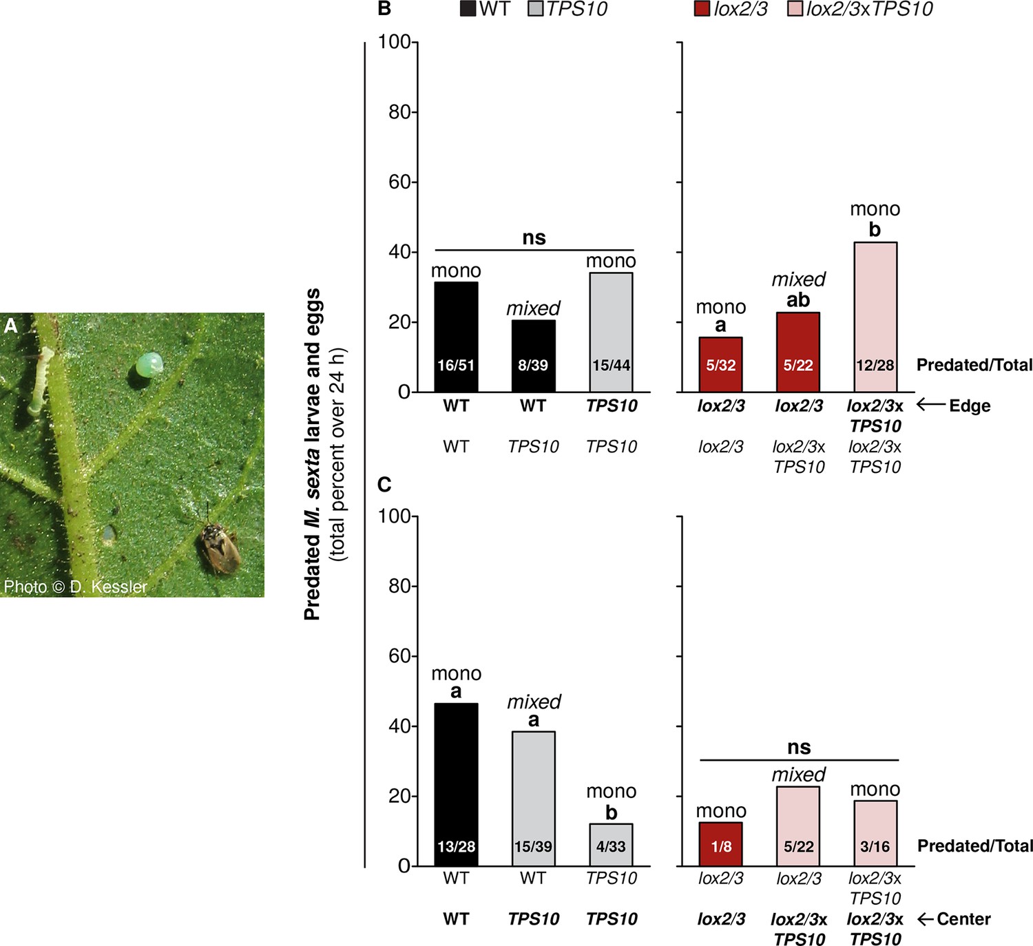
TPS10 and LOX2/3 interact to alter the predation of M. sexta by Geocoris spp from edge vs center plants.
(A) Photograph of a M. sexta egg and first-instar larva, and G. pallens adult on an N. attenuata leaf reprinted with permission from Danny Kessler, Copyright 2006. All rights reserved. As shown here, one first-instar M. sexta larva and one egg were placed on a lower stem leaf in a standardized position on healthy, size-matched plants (one leaf/plant), and their predation was monitored for 24 hr. Data are total numbers from five consecutive trials conducted between June 21st and June 27th at the end of experimental season two, when Geocoris spp. and herbivores were more abundant (see Figure 5). (B and C) Predation rates of M. sexta are higher on lox2/3xTPS10 than lox2/3 plants at the edges of monocultures (B), but lower on TPS10 than WT plants at the centers of monocultures (C). Bars indicate the total percentage of M. sexta eggs and larvae predated per population; numbers of predated/total eggs and larvae are given inside bars. The same trends were observed in both egg and larva predation; separate numbers of larvae and eggs predated are given in Figure 11—source data 1. Plants of the WT background and plants with the lox2/3 silencing construct were separately matched for parallel experiments and thus analyzed separately. (B) Predation of herbivores from edge plants was similar (not significant, ns) regardless of the number of TPS10 plants in WT + TPS10 populations, but increased with increasing numbers of lox2/3xTPS10 plants in lox2/3 + lox2/3xTPS10 populations. For plants at the center of populations, the pattern was reversed: (C) predation rates decreased with increasing numbers of TPS10 plants in WT + TPS10 populations, and were similar (ns) regardless of the number of lox2/3xTPS10 plants in lox2/3 + lox2/3xTPS10 populations. a,b Different letters indicate significant differences (corrected p<0.05) in Fisher's exact tests; p-values were corrected for multiple testing using the Holm-Bonferroni method.
-
Figure 11—source data 1
Total numbers of M. sexta larvae and eggs predated by Geocoris spp. in experimental season two (corresponding to data shown in Figure 10).
- https://doi.org/10.7554/eLife.04490.026
TPS10-expressing plants significantly altered predation rates at the edges and centers of populations, and whether the effect was at the edge or the center depended on LOX2/3 expression (Figure 11B,C). Specifically, TPS10 expression increased predation from edge plants in lox2/3 and lox2/3xTPS10 populations (Fisher's exact tests, corrected p-values<0.05) but not in WT and TPS10 populations (21–34%, corrected p-values >0.3) (Figure 11B). At the edges of monocultures, lox2/3xTPS10 plants received 43% predation whereas lox2/3 plants received only 16% (corrected p=0.049), and lox2/3 plants at the edges of lox2/3 + lox2/3xTPS10 mixed cultures were intermediate with 23% (lox2/3 mono v. lox2/3 + lox2/3xTPS10 mixed, corrected p=0.723, lox2/3xTPS10 mono v. lox2/3 + lox2/3xTPS10 mixed, corrected p=0.457). On the other hand, TPS10 expression decreased, rather than increased predation from center plants in WT + TPS10 populations (from 46% to 12%, corrected p<0.04) and had no effect on center plants in LOX2/3-deficient populations (ranging from 13% to 23%, corrected p-values=1, Figure 11C). WT plants received 46% predation at the center of monocultures, while TPS10 plants received 38% predation at the center of mixed cultures and only 12% at the center of monocultures (WT mono v. WT + TPS10 mixed, corrected p=0.618; WT mono v. TPS10 mono, corrected p=0.012; WT + TPS10 mixed v. TPS10 mono, corrected p=0.031).
Thus in populations of lox2/3 and lox2/3xTPS10 plants deficient in all HIPVs except for the engineered TPS10 volatiles, TPS10 expression by edge plants increased predator activity on those plants. In contrast, TPS10 expression by center plants failed to attract more predator activity to the centers of populations. In populations of WT and TPS10 plants with intact WT HIPVs, TPS10 expression did not increase predator activity at all; however, TPS10 expression by edge plants seemed to reduce the penetration of predators to center plants. Thus, depending the richness of the plants' HIPV blends, TPS10 expression had either positive direct effects on predator activity for emitting plants, or negative indirect effects for their neighbors.
Discussion
In this study, we sought to fulfil the four postulates of community genetics (Wymore et al., 2011; Whitham et al., 2012) to uncover the community effects of genes controlling direct and indirect defenses in the wild tobacco N. attenuata. N. attenuata has already been shown to fulfill postulate one: significantly affecting an ecological community of other plants and animals, and native microbes (reviewed in Schuman and Baldwin, 2012; see also Long et al., 2010; Meldau et al., 2012; Machado et al., 2013; Santhanam et al., 2014). Postulate two, demonstration of genetically based traits, is ensured by our method of altering the expression of specific genes: LOX2, LOX3, and TPS10 (Figure 1 and associated source data files, Appendices 1, 2). Thus, we created transgenic lines from a single genotype of N. attenuata and used them to investigate both individual- and population-level effects of two HIPVs, (E)-α-bergamotene (TAB) and (E)-β-farnesene (TBF), produced by the sesquiterpene synthase TPS10, in plants which either had wild-type direct defenses and HIPVs, or reduced production of direct defenses and other HIPVs. We used these plants to evaluate postulate three: different effects on community processes of conspecifics differing in LOX2/3 and TPS10 expression, and postulate four: predictable effects on those community processes when the genes are manipulated.
Specifically, we found that LOX2/3-mediated defense had a strong and direct effect on plant resistance to foliar herbivores and plant mortality (Figures 4, 5 and associated source data files, Figure 9), as predicted (Kessler et al., 2004). Interestingly, the effect of LOX2/3 expression on herbivore abundance was less clear: LOX2/3 deficiency was associated with significantly increased herbivore abundance for edge plants in populations, but not overall (Figure 6). Furthermore, although TPS10 expression did not significantly affect foliar herbivore damage or performance, it did consistently reduce foliar herbivore abundance (Figure 6). It should be noted that the herbivore damage data in Figure 5B were collected just over 2 weeks earlier than the herbivore abundance data in Figure 6; however, the relative amounts of damage on plants at the time that herbivore abundance data were collected still reflected the patterns shown in Figure 5, with LOX2/3-deficient genotypes having visibly more damage and WT and TPS10 plants not differing visibly in herbivore damage levels.
More surprisingly, we found population-level effects of TPS10 volatiles which were as great as the individual-level effects of total LOX2/3-mediated defenses, and dependent on LOX2/3 expression. Single TPS10-expressing plants reduced the mortality of plants in LOX2/3-deficient populations (Figure 9), corresponding to an increase in apparent health of those plants. Additionally, TPS10 expression significantly increased the infestation rate of neighbors by the stem-boring weevil T. mucorea (Figure 10), and TPS10 expression in a population strongly altered the distribution of predation services among edge and center plants, depending on LOX2/3-mediated defense (Figure 11 and associated source data file).
It should be noted that our experimental design did not support the analysis of population-level effects resulting from changing LOX2 and LOX3 expression in single members of a population. Had we included these treatment groups as well (e.g., populations with a central lox2/3 plant surrounded by WT, and with a central lox2/3xTPS10 plant surrounded by TPS10), we predict that we would also have observed significant neighbor effects of LOX2/3 expression in populations. However, given the magnitude of direct effects of LOX2/3 expression, it would be surprising if the indirect population-level effects from manipulating LOX2/3 expression in single plants were larger than the direct effects—as was generally observed from the manipulation of TPS10 expression. Our experiment was designed to determine whether TPS10 products have direct and neighbor effects in the presence, or absence, of total HIPVs and jasmonate-mediated defense.
We found no effects on non-target metabolites, (Figure 1—source data 3, Appendix 2), and only minor effects on plant size and growth which were all associated with the alleviation of the costs of LOX2/3-mediated defense for single plants, benefits which disappeared under high herbivory loads (Figures 7, 8 and associated source data file, Schuman et al., 2014).
Plant productivity depends on herbivore damage rates, LOX2/3 and TPS10 expression
It is well known that jasmonate-mediated defenses can be costly in the absence of herbivores (reviewed in e.g., Steppuhn and Baldwin, 2008), and under low levels of damage from herbivores in season one (Figure 5A), growth and early flower production was greater in lox2/3 and lox2/3xTPS10 than in WT and TPS10 plants (Figures 7, 8 and associated source data file). These data indicate that our measurements were sufficiently sensitive to detect developmental costs of defense metabolite production. Attempts to engineer the emission of terpene volatiles have sometimes resulted in plants with stunted growth or symptoms of autotoxicity (Robert et al., 2013; reviewed in Dudareva and Pichersky, 2008; Dudareva et al., 2013). However, we did not detect any consistent costs of TPS10 overexpression: TPS10 plants were generally not smaller than WT (Figure 8 and associated source data file). The same line of TPS10 also grew similarly to WT in a greenhouse competition study (line 10–3 in Schuman et al., 2014).
However, there were effects of TPS10 expression on flowering which differed depending on plants' position in different populations. In particular, under high herbivory in season two, TPS10 expression strongly decreased flower production for well-defended individual plants, but promoted flower production in LOX2/3-deficient individuals (Figure 8B). In contrast, flower production was not affected by TPS10 expression for edge plants in populations, and was slightly reduced for TPS10-expressing plants in the centers of populations (Figure 8D,F). For central plants, in contrast to individuals, the reduction in flower production due to TPS10 expression was similar both for LOX2/3-expressing and LOX2/3-deficient plants. Overall, these data indicate that TPS10 expression may have altered the relative attractiveness or apparency of TPS10 plants, with results depending strongly on plants' neighbors. The potential mechanisms in terms of herbivore abundance and predation rates, and consequences in terms of health and mortality, are discussed further below.
Higher levels of damage from foliar herbivores in season two (Figure 5B) were likely the main factor which shifted LOX2/3-mediated defenses from costly, in terms of early flower production (Figure 7), to beneficial, in terms of reduced plant mortality before and during the reproductive phase, and increased apparent plant health (Figure 9 and Figure 9—figure supplement 1). Overall, there were few differences in growth and size among genotypes (Figure 8 and associated source data file, and results reported in text), making it reasonable to attribute changes in herbivore damage, mortality, and other interactions to the manipulated chemical traits, rather than plant apparency or attractiveness based on size and development.
LOX2/3 expression has large direct effects on plants, while TPS10 expression has large indirect effects
LOX2/3 deficiency significantly increased damage from foliar herbivores and growth of the specialist M. sexta, whereas TPS10 expression had no effect on either interaction (Figures 6, 7). There was, furthermore, no effect of plant population type (mixed or monoculture) on damage from foliar herbivores in field experiments (Figure 5 and associated source data files). Together, these data indicate that feeding of M. sexta larvae and other naturally occurring foliar herbivores are not directly affected by TPS10 volatiles. However, TPS10 volatiles may have altered the attraction of herbivores to plants: TPS10-expressing plants had consistently smaller populations of foliar herbivores by the end of season two, despite the fact that these plants tended to look healthier, and independently of LOX2/3 expression (Figure 6). In contrast, ovipositing T. mucorea mothers may be attracted to TPS10 volatiles (Figure 10). Interestingly, M. sexta moths laid fewer eggs on plants for which the headspace had been supplemented with TAB (Kessler and Baldwin, 2001). A direct effect on colonizing herbivores and ovipositing females may result in indirect effects in terms of associational resistance or associational susceptibility for neighboring plants (Kessler and Baldwin, 2001; Barbosa et al., 2009). Although such indirect effects were not detected in foliar herbivore abundance on neighboring WT and lox2/3 plants (Figure 6C), TPS10 expression did significantly affect neighbors' mortality (Figure 9), apparent health, infestation by T. mucorea larvae (Figure 10), and predation services (Figure 11).
The most straightforward indirect effects of TPS10 expression were evident in open headspace trappings (Figure 3): the presence of a lox2/3xTPS10 plant in the center of a population was associated with TAB in the headspace of neighboring lox2/3 plants, and TAB was not found in the open headspaces of lox2/3 individuals or monocultures. The most parsimonious explanations are diffusion of volatiles into neighbors' headspace, or adherence and re-release of volatiles from the surface of neighbor plants, as has been shown in birch (Betula spp.) by Himanen et al. (2010). Because no TAB was detectable in extracts from the leaves of lox2/3 plants even when plants were much larger and more likely to have direct contact with TPS10 neighbors, it is unlikely that the TAB detected in open trappings of lox2/3 headspaces came from the stimulation of TAB biosynthesis in lox2/3 (Figure 1C, Figure 1—source data 3).
Indirect effects of TPS10 volatiles on neighboring plants may be attributed to the volatile compounds themselves, because we found no evidence that TPS10 volatiles affected the defenses of emitting plants, or of neighbor plants in populations (Appendices 1, 2, Figure 1 and associated source data files); and TPS10 plants also did not alter the defense response of neighbors in a glasshouse competition experiment (Schuman et al., 2014). In contrast, due to the large suite of defenses regulated by LOX2 and LOX3 products, it would have been more difficult to determine the proximate cause of neighbor effects resulting from manipulation of LOX2 and LOX3 expression. Although several components of plant HIPV blends have been shown to prime the direct and indirect defenses of neighbors in different systems (reviewed in Baldwin et al., 2006; Arimura et al., 2010; see Heil and Kost, 2006), GLVs may often be the active cues (Engelberth et al., 2004; Kessler et al., 2006; Frost et al., 2008). We did not mix GLV-deficient with GLV-emitting plants in our experimental design, but we can conclude that TPS10 volatiles had no detectable direct effects on neighbor plants in our set-up.
Indirect effects of TPS10 HIPVs may benefit or harm emitters, depending on the emission and LOX2/3-mediated defense levels of their neighbors
We observed multiple significant indirect effects of TPS10 expression in populations, as mentioned above; and two of these were strongest in mixed cultures containing only one TPS10-expressing plant. The mortality of lox2/3 and lox2/3xTPS10 plants in monocultures was significantly higher than that of WT and TPS10 plants in monocultures, but the mortality of lox2/3 + lox2/3xTPS10 plants in mixed cultures was not higher than that of WT + TPS10 plants in mixed cultures (Figure 9). Thus, a single TPS10 emitter in populations of otherwise defenseless plants reduced overall mortality to levels comparable to well-defended populations containing single TPS10 emitters. This apparent protective effect of TPS10 volatiles was weaker for monocultures of lox2/3xTPS10 plants. This may be because TPS10 volatile emission makes plants more apparent to herbivores like T. mucorea as well as beneficial insects like Geocoris spp. (Figures 9, 10), and if plants are otherwise poorly defended, greater apparency may be dangerous (Feeny, 1976). Interestingly, although there were no statistically significant differences in mortality among populations of WT and TPS10 plants, mortality was lowest in TPS10 monocultures; and WT + TPS10 mixed cultures had mortality rates 1.5-fold that of TPS10 monocultures (Figure 9). This indicates that well-defended TPS10 plants may have benefited directly from emitting TPS10 volatiles, and may have additionally increased the mortality of non-emitting neighbors. If so, TPS10 volatiles may increase plants' competitive ability by increasing neighbor mortality.
Indeed, TPS10 plants had a dramatic effect on the infestation of their WT neighbors by T. mucorea weevils (Figure 10). TPS10 volatiles seemed only to affect the infestation rates of plant populations; for individual plants, jasmonate-mediated defense is likely more important (Diezel et al., 2011, and see ‘Results’). Infestation patterns in populations (Figure 10) strongly indicate that ovipositing T. mucorea adults seek populations of plants based on their volatile emission and then oviposit on all plants in the population. Infestation rates did tend to be higher for lox2/3xTPS10 plants than for lox2/3 plants in populations (Figure 10C), indicating that the absence of other volatiles such as GLVs may reduce plants' apparency to ovipositing T. mucorea.
It is interesting that the TPS10-mediated increase in T. mucorea infestation was greater for WT plants in mixed WT + TPS10 populations than for TPS10 plants in monocultures (Figure 10): though TPS10 monocultures tended to have higher infestation rates than WT monocultures, this difference was not statistically significant, whereas the difference between WT plants in monocultures and WT plants in mixed cultures was both larger and significant. It is tempting to speculate that T. mucorea may be attracted to lower relative abundance of TPS10 volatiles, and deterred by higher relative abundance of these volatiles in the total mixture of the plant headspace. If true, this could provide a mechanism by which TPS10 emitting plants could inflict an indirect cost of emission on non-emitting neighbors, which would be always slightly higher than their own cost of emission. Furthermore, if attraction or deterrence depended on the ratio of TPS10 volatiles to other plant volatiles, the effects might differ for TPS10 and lox2/3xTPS10 plants (Bruce et al., 2005).
The infliction of such an indirect cost on neighbors is reminiscent of extortionist strategies in the iterated prisoner's dilemma of evolutionary game theory: extortionist strategies lock a player's payoff to its opponent's payoff plus some positive number, thereby ensuring that the extortionist always benefits compared to its opponent (Press and Dyson, 2012). Interestingly, such strategies have been shown in simulations not to be evolutionarily stable, but to catalyze the evolution of cooperation in populations (Hilbe et al., 2013). Of course it is possible that the manipulation of LOX2 and LOX3 expression within populations would also reveal such extortionist-like effects, for example if T. mucorea preferred to oviposit in TPS10 plants over lox2/3xTPS10 plants in the same population, which would support the hypothesis that T. mucorea preference reflects the ratio between TPS10 volatiles and other HIPVs.
Effects of TPS10 volatiles on indirect defense depend on LOX2/3-mediated direct and indirect defense
Predation rates of M. sexta herbivores from edge and center plants in populations (Figure 11) indicate that populations' total HIPV emissions can alter the roles of specific volatiles for indirect defense. In lox2/3 + lox2/3xTPS10 populations, deficient in all HIPVs except those provided by TPS10 expression, lox2/3xTPS10 edge plants of monocultures experienced higher predation rates, whereas predation rates were similar for center lox2/3xTPS10 and lox2/3 plants in mono- and mixed cultures. For TPS10 and WT plants, effects on predation rates were exactly the opposite. There was significantly less predation of M. sexta from TPS10 center plants in monocultures vs mixed cultures, but TPS10 edge plants had predation rates similar to WT. Together, these results indicate that the effect of TPS10 volatiles on indirect defense was positive for lox2/3xTPS10 plants, but negative for TPS10 plants, and only significant for plants in monocultures. In mixed cultures, TPS10 volatiles had no effect on the predation of M. sexta herbivores from emitting plants or their neighbors. It should be noted that due to higher mortality in lox2/3 + lox2/3xTPS10 populations, center plants were sometimes more exposed in these populations as a result of edge plants dying. However, the fact that TPS10 volatiles benefitted only edge plants in these populations indicate that Geocoris spp. predators nevertheless distinguished between edge and center plants.
We conclude that TPS10 expression had different consequences for plants' indirect defense, depending on whether one or all plants in a population expressed TPS10, and whether those plants also emitted other HIPVs. If only one plant in the population expressed TPS10, or if other HIPVs were also emitted in the population, TPS10 expression did not enhance indirect defense and was sometimes detrimental to emitters. The attraction of most, or all, predators and parasitoids to HIPVs depends on learned associations between HIPVs and prey: naïve predators are just as likely to respond as they are not to respond (Allison and Hare, 2009). Because LOX2/3-deficient plants were heavily attacked by herbivores (Figure 5), predators could associate TPS10 volatiles emitted by lox2/3xTPS10 plants with herbivore damage (though damage did not necessarily reflect abundance—see Figure 6). Because lox2/3 and lox2/3xTPS10 plants had reduced emissions of other HIPVs (Figure 1 and associated source data files, Appendix 2), there were few other volatiles which could provide the basis for learned associations between HIPVs and prey. On the other hand, TPS10 volatiles emitted constitutively by less heavily attacked TPS10 plants (Figure 5) would be less often associated with feeding herbivores than the endogenous HIPVs released only when herbivores attack, and all the more so if TPS10-expressing plants supported fewer foliar herbivores (Figure 6). Perhaps because ‘honest’ endogenous HIPVs were also emitted by WT plants, TPS10 plants had no advantage over WT in attracting predators.
The concept of honest vs deceptive, or ‘cry wolf’ HIPV emission has been investigated in the context of emission proportionate, or disproportionate to numbers of attacking herbivores (Shiojiri et al., 2010). But what happens when plants ‘cry wolf’ by constitutively emitting volatiles which, in nature, are only associated with herbivore damage? Plants engineered to constitutively emit particular HIPVs can attract more parasitoids when parasitoids are trained to associate engineered volatiles with their prey (Kappers et al., 2005; Schnee et al., 2006), or when all emitting plants are also experimentally infested (Rasmann et al., 2005; Degenhardt et al., 2009). Such studies demonstrate that genetic engineering of HIPVs can enhance indirect defense, but they do not demonstrate that constitutive emission is an effective strategy in the complex environments of agriculture, or nature (Kos et al., 2009; Schuman et al., 2012; Xiao et al., 2012). From an arthropod's perspective, constitutive HIPV emission is oxymoronic. If there is no effort to artificially associate constitutively emitted volatiles with prey, predators, and parasitoids may not learn to respond, or worse, learn to actively ignore the volatile emissions. Whether achieved via genetic methods or synthetic release stations (Kaplan, 2012), constitutive emission is unlikely to enhance indirect defense if prey densities are low, or if plants emit other ‘honest’ HIPVs.
Moreover, assigning an indirect defense function to HIPVs based on their ability to attract predators or parasitoids to single plants may be misleading. In real populations, the effectiveness of HIPVs likely depends on the density of HIPV emission and the location of emitting plants (Xiao et al., 2012). There may be competition among plants in populations either to attract, or to arrest predators and parasitoids of herbivores. Specifically, whether plants benefit from emitting more or less than their neighbors likely depends on the basal level of HIPV emission in a population (low or high), and the location of plants in a population (edge or center). Perhaps, wild-type plants are capable of adjusting their own volatile emission in response to the emission of their neighbors in order to adapt (Choh et al., 2004; Baldwin et al., 2006; Yan and Wang, 2006). In this context, it would be interesting to know whether central lox2/3 plants surrounded by WT edge plants would experience a similar predation disadvantage as central TPS10 plants surrounded by WT edge plants, and whether central WT plants surrounded by lox2/3 edge plants would have an advantage over their neighbors in attracting predators.
Conclusion
Now that careful and extensive research has established the importance of biodiversity to ecosystem function, the next step is to understand how the two are linked in order to craft informed socioeconomic and environmental policy (Midgley, 2012). The community genetics perspective is essential in order to understand biodiversity effects at the level of individual heritable traits (Whitham et al., 2006). This is especially true in light of recent research showing that intraspecific, genetic biodiversity is at least as important as interspecific biodiversity for the structure of ecological communities (Crutsinger et al., 2006; Johnson et al., 2006; Cook-Patton et al., 2011; Moreira and Mooney, 2013) and the recognition that interspecific biodiversity is an emergent property of genetic biodiversity (Johnson and Stinchcombe, 2007; Haloin and Strauss, 2008).
The work presented here demonstrates that the population-level effects of an indirect defense gene may be greater than its effects on individual plants, demonstrating that the population perspective is vital to our understanding of gene function. Furthermore, our results indicate that populations comprising individuals differing in only a single genetic trait can functionally imitate more diverse communities. Engineering functional diversity may become an important strategy in a world with over 10 billion humans (United Nations, Department of Economic and Social Affairs, Population Division, 2013), where every patch of arable land may be planted with custom-engineered high-yield crop monocultures.
Materials and methods
WT and transgenic plant lines and glasshouse growth conditions
Request a detailed protocolSeed germination, glasshouse growth conditions, and the Agrobacterium tumefaciens (strain LBA 4404)–mediated transformation procedure have been described previously (Krügel et al., 2002; Schuman et al., 2014). Seeds of the 31st generation of the inbred ‘UT’ line of N. attenuata (Torr. ex S Watson) described by Krügel et al. (2002) were used for the wild-type (WT) plants in all experiments. We used homozygous transformed lines of the second transformed generation (T2), each with a single transgene insertion, to either ectopically overexpress Zea mays TERPENE SYNTHASE 10 (TPS10) under the control of a 35S promoter in the pSOL9 plasmid (TPS10 line A-09-389-6/10-3, described in Schuman et al., 2014), or silence N. attenuata LIPOXYGENASE 2 and LIPOXYGENASE 3 (LOX2/3) via an inverted repeat construct specifically targeting both genes in the pSOL8 plasmid (line A-07-707-2, sequences targeting NaLOX2 and NaLOX3 described in Allmann et al. (2010) (Figure 1). Vector construction and the pSOL8 and pSOL9 plasmids have been described previously (Gase et al., 2011). To combine the ectopic overexpression of TPS10 with the silencing of LOX2/3, a hemizygous cross was created between the lox2/3 and TPS10 T2 homozygous lines (lox2/3xTPS10, Figure 1). Further details of transgenic line screening and characterization are given in Appendix 3.
Field plantations and growth conditions
Request a detailed protocolFor field experiments, seedlings were transferred to 50 mm peat pellets (Jiffy) 15 days after germination and gradually hardened to the environmental conditions of high sunlight and low relative humidity over 10 days. Small, adapted, size-matched rosette-stage plants were transplanted into a field plot in a native habitat in Utah located at latitude 37.146, longitude 114.020. Field plantations were conducted under APHIS permission numbers 06-242-3r-a3, 10-349-102r, and 11-350-101r. Plants were watered thoroughly once at planting and as needed over the first 2 weeks until roots were established; all plants received the same watering regime in each year. WT, TPS10, lox2/3, and lox2/3xTPS10 plants were arranged as individuals and populations according to the descriptions in Figure 2 and Figure 2—figure supplement 2 (n = 12 in season one, n = 15 in season two of each individual or population type).
A distance of 0.5 m is sufficient for N. attenuata's herbivores and their predators to distinguish odor from individual plants (Kessler and Baldwin, 2001; Schuman et al., 2012): so that insects could perceive plants in a population as a single unit, they were planted in 0.4 × 0.4 m squares, while the distance between single individuals/populations was ca. 1.5 m. Individual and population types were marked with small (ca. 5 cm long, ⌀ 0.5 cm) bamboo sticks having different numbers of horizontal markings, which were checked during experiments only when establishing treatment groups, or confirming current location within the experiment. During experiments and data collection, plants were referred to only by their number or position (e.g., n1 population 2 upper left, where upper left was defined from a standardized observer position). Plant genotypes were never identified during data collection to avoid bias, and experimental treatments and data collection were spatially and temporally randomized corresponding to the randomized arrangement of individuals and populations in the field plot (Figure 2—figure supplement 2).
Tissue samples from glasshouse- and field-grown plants
Request a detailed protocolPrior to measuring gene transcripts and induced defenses or HIPVs, glasshouse-grown plants, which were not damaged by herbivores, were treated with wounding and M. sexta oral secretions (W + OS) as a standardized method to mimic herbivore feeding as described previously (Schuman et al., 2012). The first fully-expanded leaf (node +1) was used for quantifying gene transcript (LOX2, LOX3, TPS10) and jasmonate (JA, JA-Ile) accumulation on a set of bolting plants. The adjacent older leaf (node +2) was used to measure headspace volatiles on the same plants (data in Appendix 2, and see ‘Quantification of volatiles in the headspace of glasshouse-grown plants’). A separate set of plants was used following the same procedure for WT and TPS10 jasmonates and GLVs, and the results are reported in Schuman et al. (2014) and ratios to WT are shown in Figure 1B. Control plants were left untreated. Treated leaves, and leaves at the same position on control plants were cut at the petiole and wrapped in a double layer of aluminum foil, then immediately flash-frozen in liquid nitrogen, and kept at −80°C until processing and analysis.
For field-grown plants, five similar, mature, non-senescent stem leaves were harvested after the end of predation assays, on June 28th of experimental season two. Two of these leaves had been damaged by the M. sexta first-instar larvae used for predation assays, and three were systemic leaves with similar levels of damage from other naturally-occurring herbivores. Leaves were cut at the petiole, pooled in a single sample per plant and wrapped in a double layer of aluminum foil, then immediately frozen on dry ice insulated with ice packs frozen at −20°C. Samples were stored at −20°C until transport to the MPICE on dry ice, where they were kept at −80°C until processing and analysis.
All sample processing was carried out over liquid nitrogen until the addition of the extraction solvents. Prior to analysis, entire leaves were crushed with a mortar and pestle and each transferred to a 2 mL microcentrifuge tube for storage. For specific measurements, aliquots were weighed into microcentrifuge tubes containing two steel balls and finely ground in a GenoGrinder (SPEX Certi Prep, Metuchen, NJ) prior to extraction.
Quantification of JA and JA-Ile in leaf tissue
Request a detailed protocolJA and the active jasmonate hormone JA-Ile were extracted from 100 mg of leaf tissue (from n = 4 plants) using ethyl acetate spiked with internal standards (IS) and quantified by LC-MS/MS (Varian, Palo Alto, CA) as described by Oh et al. (2012), with the modification that 100 ng rather than 200 ng of [2H2]JA, and 20 ng rather than 40 ng of JA-[13C6]Ile were used as internal standards (IS). Individual jasmonates were quantified in ng by comparison to the corresponding IS peak area and normalized per g leaf tissue fresh mass (FM). The quantification of TPI in field tissue samples as an indicator of jasmonate signaling is described in Appendix 3.
Quantification of volatiles in the headspace of glasshouse-grown plants
Request a detailed protocolFor GLVs, the +2 leaf (n = 4 plants) was enclosed immediately after W + OS elicitation in two 50 mL PET cups (Huhtamaki, Finland) lined on the edges with foam to protect leaves and with an activated charcoal filter attached to one side for incoming air, and secured with miniature claw-style hair clips as described previously (Schuman et al., 2009). For TPS10 products in the headspace of glasshouse-grown plants (n = 4), leaves were enclosed 24 hr after W + OS treatment and the headspace was collected from 24–32 h during the peak emission of sesquiterpenes in N. attenuata (Halitschke et al., 2000). Headspace VOCs were collected on 20 mg of Poropak Q (Tholl et al., 2006; Sigma–Aldrich, St. Louis, MO) in self-packed filters (bodies and materials from ARS Inc., Gainesville, FL) by drawing ambient air through these clip cages at 300 mL min−1 using a manifold with screw-close valves set to provide equal outflow, via pushing air at 2 to 3 bar through a Venturi aspirator as described previously (Oh et al., 2012). Background VOCs present in ambient air were collected using empty trapping containers and background signals were later subtracted if necessary from raw intensities of plant samples prior to further processing.
After trapping, Porapak Q filters were stored at −20°C until extraction by addition of 320 ng of tetralin as an internal standard (IS), and elution of volatiles with 250 mL of dichloromethane (Sigma–Aldrich). Filters were eluted into a GC vial containing a 250 μL glass insert. Samples were analyzed on one of two different GC–MS instruments from Varian with columns from Phenomenex (Torrance, CA; 30 m × 0.25 mm i.d., 0.25 μm film thickness). 1 μL of each sample was injected in splitless mode, and then the injectors were returned to a 1:70 split ratio from 2 min after injection through the end of each run. He carrier gas was used with a column flow of 1 mL min−1. GLV samples were analyzed by a CP-3800 GC Saturn 2000 ion trap MS with a polar ZB-wax column and a CP-8200 autoinjector; the GC and MS were programmed as previously described for this instrument (Schuman et al., 2012), and compounds were separated by a temperature ramp of 5°C min−1 between 40°C and 185°C. TPS10 products and other VOCs were analyzed on a CP-3800 GC coupled to a Saturn 4000 ion-trap mass spectrometer with a nonpolar ZB5 column and a CP-8400 autoinjector; The GC and MS were programmed as previously described for this instrument (Oh et al., 2012), and compounds were separated by a temperature ramp of 5°C min−1 between 40°C and 180°C.
Individual volatile compound peaks were quantified using the combined peak area of two specific and abundant ion traces per compound using MS Work Station Data Analysis software (Varian) and normalized by the 104 + 132 ion trace peak area from tetralin in each sample. The identification of compounds was conducted by comparing GC retention times and mass spectra to those of standards and mass spectra databases: Wiley version 6 and NIST (National Institute of Standards and Technology) spectral libraries.
The area of trapped leaves was quantified for comparison by scanning and calculating areas in pixels using SigmaScan (Systat Software Inc., San Jose, CA), and subsequently converting pixels to cm2 using a size standard which was scanned with leaves.
Quantification of plant volatiles in hexane extracts of field tissue samples
Request a detailed protocolPlant volatiles were quantified in tissue from field-grown plants (n = 9–22). Frozen tissue (100 mg) was spiked with 800 ng tetralin as an internal standard (Sigma–Aldrich) and extracted in 300 µL hexane during an overnight rotating incubation at RT. Tissue was allowed to settle and 100 µL of water- and tissue-free hexane was transferred to a GC vial containing a 250 µL microinsert. Samples were analyzed by a Varian CP-3800 GC-Saturn 4000 ion trap MS connected to a ZB5 column (30 m × 0.25 mm i.d., 0.25 μm film thickness; Phenomenex) as described in ‘Quantification of volatiles in the headspace of glasshouse-grown plants’. Analyte quantities were expressed as percent tetralin IS per 100 mg FM.
Quantification of volatiles in the open headspace of field-grown plants
Request a detailed protocolFor the data in Figure 3, on May 16th of season two, four activated charcoal filters were placed around each plant (n = 4) as shown in Figure 3A and the headspace was not enclosed. The open headspace was sampled for 7 h during the day at which time emission of most volatiles was previously found to be greatest (Appendix 2). After elution (see Appendix 3), eluents from all four filters were combined and concentrated to a volume of 15–20 µL under a gentle stream of nitrogen gas. Pooled and concentrated samples were analyzed by Agilent 6890N GC equipped with an Agilent 7683 auto-injector coupled with a LECO (St. Joseph, MI) Pegasus III time-of-flight MS with a 4D thermal modulator upgrade. Injected samples were separated first on a nonpolar column (C1 RTX-5MS, 20 m × 250 µm i.d. × 0.5 µm; Restek, Bellefonte, PA) and every 6 s (modulation time) transferred to a midpolar column (DB-17, 0.890 m × 100 µm i.d. × 0.1 µm; Agilent Technologies, Santa Clara, CA) for the second separation. Chromatography and analysis conditions as well as deconvolution, alignment, and integration of VOC analyte peaks are described in Gaquerel et al. (2009). During peak table alignment using the comparison feature imbedded in ChromaToF software (LECO), mass spectra alignment was accepted at a similarity threshold of 500/1000. Individual volatile compound peaks were normalized by the peak area of the tetralin IS in each sample. Analyte quantities were expressed as percent tetralin IS per plant.
Measurement of M. sexta growth
Request a detailed protocolAs for OS collection, we used M. sexta neonates from an in-house colony at the MPICE. One M. sexta neonate per plant was placed on the youngest rosette leaf of elongated plants (n = 25 larvae). Larval movement was unrestricted within a plant, but plants were spaced on the table so that larvae could not move directly between plants. Larval mass was determined on days 8 and 12, corresponding on average to the third and fourth larval instars. Plant genotypes were randomized spatially on a single glasshouse table and temporally in placement and weighing of larvae. Due to mortality and to larval movement off of plants, 11–16 larvae remained within each treatment group by day 12.
Assessment of foliar herbivore damage
Request a detailed protocolTotal canopy damage due to herbivores occurring naturally on the field plot was quantified on June 9th in season one, and on June 2nd in season two. Damage was calculated as described in Schuman et al. (2012) by identifying damage from specific herbivores according to their characteristic feeding patterns, counting the number of leaves per plant (small leaves were counted as 1/5 to 1/2 of a leaf based on leaf area and large leaves were counted as 1 leaf), estimating the total percentage of leaf area damage due to each herbivore, and dividing the total leaf area damage from each herbivore by the total number of leaves. Leaf area damage was estimated in categories of 1%, 5%, 10%, 15%, and so on, in steps of 5%. All such damage estimates were made by MCS. Plants with a health index <2.5 (see ‘Ranking of apparent plant health’) were excluded from herbivore damage calculations as it was difficult to accurately assess herbivore damage to these plants.
Herbivore and predator counts
Request a detailed protocolIn the morning of June 26th in season two, a subset of focal plants with a health index ≥2 was chosen (see ‘Ranking of apparent plant health’) and numbers of herbivorous and predacious arthropods present on the shoots of these plants were counted (total n's in Figure 6—source data 1, 2). The counting was done by a team of two people in parallel moving down the plot in the same direction, so as to complete counts as quickly as possible and to avoid disturbing plants prior to counting. Plants were randomly assigned to each counter. Counting proceeded by looking at each branch of the plant in a systematic order from the top to the bottom of the plant, observing both the adaxial and abaxial sides of leaves as well as full areas of stems. In this way especially mobile arthropods which tend to feed near the top of plants were either counted before they fled (Epitrix spp.), or could be counted once they had relocated to the base of the plant (T. notatus).
Measurement of plant size and flower production
Request a detailed protocolPlant size (rosette diameter, stem length, and branching) was measured at three times during the main period of vegetative growth and beginning of reproduction in season one (May 1st–2nd, 8th–11th, and 16th–17th), and after plants had switched from vegetative growth to reproduction in season two (June 4th–6th), at which time stem diameter was also measured. Rosette diameter was measured as the maximum diameter found by gently laying a ruler over the rosette; stem length was measured from the base of the stem to the tip of the apical inflorescence by placing a ruler beside the stem resting at the base of the rosette; stem diameter was measured by placing a calipers at the base of the stem immediately above the rosette; and all side branches 5 cm or longer were counted.
Additionally, plant reproductive output was monitored by counting the number of flowers (counted once the corolla protruded visibly from the calyx) before removal at two time points after plants began to flower: on May 8th–11th and 16th–17th in season one, and on May 29th and June 4th–6th in season two. Additionally, buds >2 mm long were counted in season two. After these counts, floral meristems were removed as necessary to prevent the distribution of ripe seeds, as is required for field-released transgenic plants.
Quantification of plant mortality and infestation by Trichobaris mucorea
Request a detailed protocolPlant mortality was quantified as the number of plants which died between the end of planting, and the end of the experiment when all plants and remains were removed from the field plot. During removal of plants on June 29th in season two, we split stems open lengthwise to check for T. mucorea frass and larvae (Diezel et al., 2011). Plants were counted as infested if the main stem was hollow and filled with T. mucorea frass, or if a larva was found in such a hollow, frass-filled stem or axial branch. These counts were done by tallying totals without reference to specific plant ID's, and thus could only be analyzed using unreplicated statistical tests.
Ranking of apparent plant health
Request a detailed protocolIn season two, plant health was also ranked by MCS on a scale of 1–5 in increments of 0.5 (1, 1.5, 2, 2.5, …, 5) using the index in Figure 7C of Schuman et al. (2012): 5, healthy, <5% of shoot senescent, no chlorosis or signs of water stress; 4, 5–10% of shoot senescent and may have visible chlorosis; 3, 10–15% of shoot senescent, some water stress, up to 50% of canopy chlorotic; 2, >15% of shoot senescent, heavy water stress or visibly sick; 1, dead. This scale was sufficiently objective that several observers not directly involved in the experiment arrived independently at the same ranks, to a precision of ±0.5, to describe the health indices of randomly-chosen plants, after training on fewer than 10 example plants.
Assay of predation by Geocoris spp.
Request a detailed protocolFive consecutive predation assays were conducted between June 21st and June 27th at the end of experimental season two, when Geocoris spp. and herbivores were abundant. M. sexta eggs and larvae (total n's given in the source data file for Figure 11) were used as bait for Geocoris spp. predators as described by Kessler and Baldwin (2001) and Steppuhn et al. (2008). Native Manduca spp. did not provide sufficient synchronously oviposited eggs for trials, and so we used M. sexta eggs kindly provided by C Miles from her laboratory colony at Binghamton University, Vestal, New York. Size-matched plants with health indices ≥2 in populations were used. We treated LOX2/3-expressing (WT, TPS10) and LOX2/3-deficient (lox2/3, lox2/3xTPS10) populations as two separate experimental groups because it was not possible to match plants across these two groups for apparent health or replicate numbers (both were lower for lox2/3 and lox2/3xTPS10 populations). During the five predation assays it was occasionally necessary to select new plants, preventing a repeated measures analysis of the predation data; however, newly selected plants were matched as described. At the end of predation assays, tissue samples were taken from a subset of these plants for the extraction of volatiles and determination of TPI activity (Figure 1, Figure 1—source data 3 and preceding methods).
For each assay, one first-instar M. sexta larva and one egg were placed on one lower stem leaf in a standardized position on each plant, and the predation of eggs and larva was monitored after 24 hr. No other Manduca spp. eggs or larvae were present on the plants used during the assays. Eggs were affixed to the underside of the leaf with a drop of α-cellulose glue (KVS, Germany), which does not damage plants or affect volatile emission (Kessler and Baldwin, 2001). Feeding by the M. sexta larva ensured the locally elicited emission of HIPVs. Larvae were considered to be predated when either the larva was missing, but clearly identifiable, fresh M. sexta feeding damage was present, or when the predated larval carcass was found on the same plant; eggs were considered predated when the eggshell was empty but intact, except for a small hole which characterizes the typical damage caused by Geocoris spp. feeding as described in Kessler and Baldwin (2001) and depicted in Figure 3 of Schuman et al. (2012). Eggs occasionally collapse during Geocoris spp. predation, but collapsed eggs were not counted unless the eggs were at least 50% empty with a visible feeding hole.
Statistical analyses
Request a detailed protocolSummary statistics were calculated in Microsoft Excel, as were G-tests, Fisher's exact tests, and tests of Spearman's correlation coefficients, which were calculated using Microsoft Excel spreadsheets from JH Macdonald's online Handbook of Biological Statistics (Macdonald, 2009). All other statistical tests were calculated in R version 2.15.2, using the RStudio interface version 0.96.316 or version 0.97.449 (R Core Team, 2012). In some cases, data which were clearly not different upon visual inspection and which had been found in similar data sets not to differ significantly were not statistically tested (e.g., rosette diameter in some subsets of data from season one).
When possible, Welch t-tests were used for pairwise comparisons and ANOVAs, linear mixed-effects models, generalized linear models, or generalized linear mixed-effects models were used for multiple comparisons as appropriate; we checked treatment groups graphically (quantile–quantile plots, residual v. fitted plots) and statistically (Shapiro–Wilk test, Bartlett test) for compliance with model assumptions, including normality and homoscedasticity. Data containing too many zero values or not meeting model assumptions were analyzed using ranking tests (Wilcoxon rank sum for pairwise comparisons, Kruskal–Wallis for multiple groups). R package nlme was used for linear mixed-effects models (Pinheiro et al., 2014), and packages lme4 (Bates et al., 2014, ; 2014b) and multcomp (Hothorn et al., 2008) were used for generalized linear mixed-effects models.
The optimal fixed structure for ANOVAs, linear mixed-effects models, generalized linear models, and generalized linear mixed-effects models was found by stepwise model simplification and factor level reduction followed by the comparison of the models via the Akaike information criterion (AIC, Akaike, 1973). Specific examples of model simplification for individual analyses are given in Appendix 3 and Figure 8—source data 1.
Holm-Bonferroni p-value corrections were calculated in Microsoft Excel for families of tests on the same data. Like the Bonferroni correction, the Holm-Bonferroni correction controls the familywise error rate and is simple to calculate, but the Holm-Bonferroni method is more powerful (Holm, 1979). Briefly, all p-values in a family of tests conducted on the same data set and subsets were listed from smallest to largest. The smallest p-value was multiplied by the total number of tests (n) conducted on that data. If the resulting corrected p-value was <0.05, then the next-smallest p-value was multiplied by n − 1. If the resulting corrected p-value was <0.05, then the third smallest p-value was multiplied by n − 2, and so on. At the first correction resulting in a p-value ≥0.05, that p-value and all larger p-values were considered non-significant. The corrected p-values reported in the text are the products of the correction procedure, for example, (smallest p-value) × n or (second smallest p-value) × (n − 1).
Appendix 1
Herbivore-induced plant defenses and HIPVs are precisely manipulated in lox2/3, TPS10, and lox2/3xTPS10 plants
We confirmed a single insertion of the inverted repeat LOX2/3 construct in several lox2/3 lines (Appendix 1—Figure 1A) and chose lines with single insertions to screen for reduced jasmonic acid (JA) and jasmonoyl isoleucine (JA-Ile) (Appendix 1—Figure 1B,C).
Based on these data, we chose lox2/3 line 707-2 for further experiments overexpressing TPS10 plants (line 10–3) also harbor a single transgene insertion (Schuman et al., 2014), and both lines were also confirmed to be diploid by flow cytometry. All transgenic lines showed the intended reduction or increase in target gene transcripts: LOX2 and LOX3 transcripts accumulated to <7% of WT levels in lox2/3 and lox2/3xTPS10, while TPS10 transcripts were easily quantifiable in TPS10 and lox2/3xTPS10, but undetectable in WT or lox2/3 (p-values < 0.01 for pairwise differences in Tukey HSD tests following p-values <0.001 in 1-way ANOVAs on natural log-transformed data, Appendix 1—Figure 2). Transcript abundance of LOX2 and LOX3 was similar in WT and TPS10 (p=1 in Tukey HSD tests) and in lox2/3 and lox2/3xTPS10 (p=0.471 for LOX2 and p=1 for LOX3); TPS10 transcript abundance was similar in TPS10 and lox2/3xTPS10 (p=0.157).
As a consequence of reduced LOX3 transcripts (Allmann et al., 2010), lox2/3 and lox2/3xTPS10 plants accumulated ≤30% of WT JA levels in a glasshouse experiment in which leaves were treated with wounding plus distilled water (W + W) or wounding plus the addition of Manduca sexta oral secretions diluted in distilled water (W + OS) to mimic herbivore attack in a precisely timed manner (Figure 1B, see also overview of phenotypes in Figure 1A). Induced levels of the active jasmonate, JA-Ile, were also reduced to <50% of WT. Absolute values for JA and JA-Ile, and significant pairwise differences in Tukey HSD tests (p-values <0.05) following two-way ANOVAs on natural log-transformed data (p-values <0.002), are shown in Figure 1—source data 1. Likewise, reduced LOX2 transcripts resulted in diminished GLV emissions from lox2/3 and lox2/3xTPS10 plants after W + W or W + OS treatment to <2% of WT levels (Figure 1B, Figure 1—source data 1). Significant pairwise differences in Wilcoxon rank sum tests (Holm-Bonferroni-corrected p-values <0.03) following Kruskal–Wallis tests (corrected p-values ≤0.020) are shown in Figure 1—source data 1. In contrast, GLV emission and JA and JA-Ile accumulation were similar in WT and TPS10 plants (Figure 1, Schuman et al., 2014), but both TPS10 and lox2/3xTPS10 plants emitted elevated amounts of TAB and TBF, more than 10-fold WT levels as measured in a second glasshouse experiment (Figure 1B, Figure 1—source data 2). Genotypes with the TPS10 overexpression construct vs those without differed significantly in their emission (Wilcoxon rank sum tests, corrected p-values ≤0.009, shown in Figure 1—source data 2).
As in the glasshouse experiments, lox2/3 and lox2/3xTPS10 plants in the field had strongly reduced jasmonate-mediated defense and GLV emission, to <4% of WT levels; and TPS10 and lox2/3xTPS10 plants emitted elevated levels of TAB and TBF, >18× WT levels (Figure 1C; data reported in the following subsection). The reductions in GLVs, JA, and JA-Ile described here for lox2/3 and lox2/3xTPS10 are similar to what has been previously reported for homozygous transformed lines silenced either in LOX2 (GLVs) or LOX3 (JA, JA-Ile) by separate, specific RNAi constructs (Allmann et al., 2010).
In summary, JA, JA-Ile, jasmonate-mediated defense, and GLVs were significantly reduced in lox2/3 and lox2/3xTPS10 plants to <4% of WT levels, and lox2/3xTPS10 and TPS10 plants produced more than 10 times as much TAB and TBF as WT or lox2/3 plants; these phenotypes were robust in plants grown under controlled glasshouse conditions and in the field (Figure 1 and supplements, Appendix 2). This set of transgenic plants (Figure 1A) allowed us to manipulate TAB and TBF independently of defense signaling and all other HIPVs, creating plants with enhanced emission in a well-defended (WT, TPS10) or poorly defended (lox2/3, lox2/3xTPS10) background.
Appendix 1—Figure 1
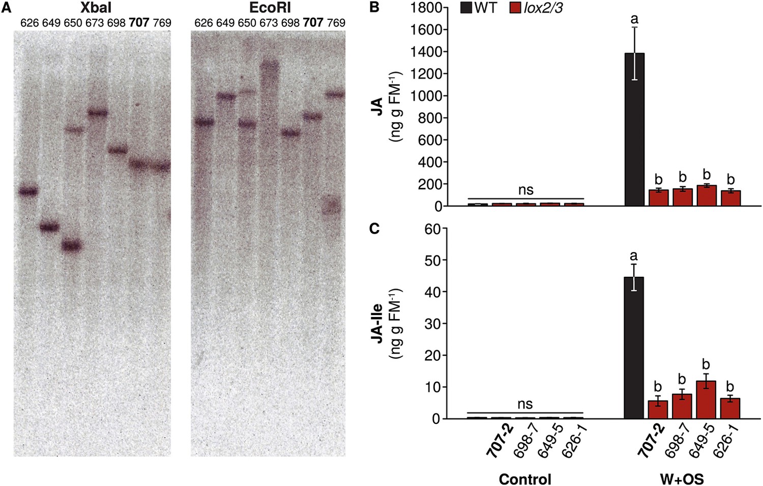
Transgene insertions and reduced jasmonate accumulation in lines of lox2/3.
(A) Southern blot of genomic DNA from multiple lines of lox2/3 digested with the restriction enzymes XbaI or EcoRI. Line 707 is highlighted: this line was used for experiments. A single transgene insertion in TPS10 (line 10–3) is shown in Schuman et al. (2014). All lines of lox2/3 screened had strong reductions in their induced (B) JA and (C) JA-Ile accumulation (mean ± SEM, n = 6). Line 707-2 was used for further experiments. a,b Different letters indicate significant differences (corrected p<0.0001) in Tukey HSD tests following significant (p<0.0001) 1-way ANOVAs on natural log-transformed data (JA: F4,25 = 54.15; JA-Ile: F4,25 = 18.00); ns, not significant in 1-way ANOVAs (p>0.4).
Appendix 1—Figure 2
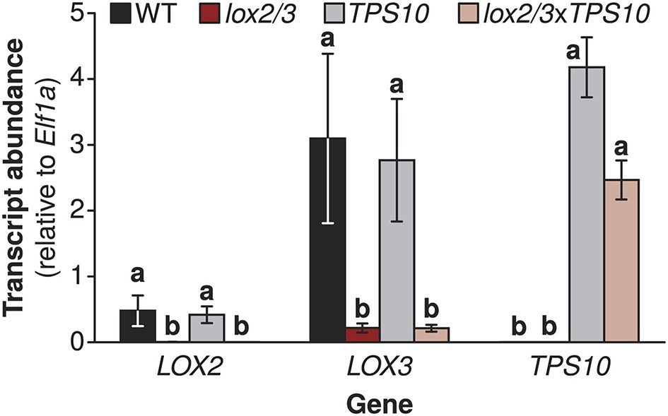
Target gene transcript levels in lox2/3, TPS10, and lox2/3xTPS10 plants.
Transcript accumulation shows that lox2/3 plants, TPS10 plants, and hemizygous crosses (lox2/3xTPS10) have the expected silencing or accumulation of the target genes LOX2, LOX3, and TPS10 (mean ± SEM, n = 4). a,b Different letters indicate significant differences (corrected p<0.01) in Tukey HSD tests following a significant (p<0.001) 1-way ANOVA on natural log-transformed data (LOX2: F3,12 = 49.49, p<0.001; LOX3: F3,12 = 13.73, p<0.001; TPS10: F3,12 = 845.6, p<0.001).
Appendix 2
Phenotypic measurements of transgenic lines in experimental field-grown populations.
Trypsin protease inhibitor (TPI) activity, a well-known jasmonate-mediated defense (van Dam et al., 2001; Halitschke and Baldwin, 2003), is more a stable trait than are JA levels in frozen tissue and thus was used as an indicator of jasmonate-mediated defense levels in field-harvested samples. TPI activity was reduced to <4% of WT activity in lox2/3 and lox2/3xTPS10 plants grown in the field. A Kruskal–Wallis test among genotypes indicated a highly significant difference (χ23 = 47.87, corrected p<0.001), as did Wilcoxon rank sum tests between WT and lox2/3, and WT and lox2/3xTPS10 (W24,12 = 0, W24,11 = 0 and corrected p-values<0.001, Figure 1C, Figure 1—source data 3). There was no significant difference in TPI activity between WT and TPS10 (W24,21 = 357, corrected p=0.065), as was previously shown in glasshouse experiments (Schuman et al., 2014).
GLV pools extracted from leaf tissue samples of field-grown lox2/3 and lox2/3xTPS10 plants were <3% of those found in leaf tissue from field-grown WT plants (corrected p-values <0.001 in Wilcoxon rank sum tests), whereas TPS10 and WT did not differ (corrected p-values = 1 in Wilcoxon rank sum tests, Figure 1C). (E)-Hexen-2-al and (Z)-hexen-3-ol were the only GLVs found in extracts (see also Schuman et al., 2012), and both differed significantly by genotype. Significant differences in pairwise comparisons between lox2/3, lox2/3xTPS10, TPS10 and WT in Wilcoxon rank sum tests (corrected p<0.001) following Kruskal–Wallis tests (corrected p-values < 0.001) are shown in Figure 1—source data 3. There was no significant effect of plant type or population type on extracted GLVs (corrected p-values =1 in Kruskal–Wallis tests across individuals, edge and center plants, or across individuals, mono-, and mixed cultures). Emission of (Z)-hexen-3-ol, the only GLV detected from plants having natural background levels of herbivore attack in season one, was also reduced in lox2/3 and lox2/3xTPS10 to <16% of WT emission (Appendix 2—Table 1). Daytime emission of (Z)-hexen-3-ol was low and differed only marginally in a Kruskal–Wallis test among genotypes (χ23 = 9.27, corrected p=0.052), but nighttime emission differed significantly in a Wilcoxon rank sum test between plants with and without the lox2/3 silencing construct (WT and TPS10 v. lox2/3 and lox2/3xTPS10, W15,15 = 171.5, corrected p=0.035). No significant effect of population type on emission was observed (Wilcoxon rank sum tests at day or night of individuals vs center plants in monocultures, corrected p-values >0.07).
Appendix 2—Table 1
Volatiles (percent IS plant−1, mean ± SEM) trapped in the headspace around single plants in experimental season one (June 8th–9th).
| GLVs (percent IS plant-1) | TPS10 products (percent IS plant-1) | Non-target volatiles (percent IS plant-1) | |||||||||||||||||||||||||||||||||||
|---|---|---|---|---|---|---|---|---|---|---|---|---|---|---|---|---|---|---|---|---|---|---|---|---|---|---|---|---|---|---|---|---|---|---|---|---|---|
| (Z)-Hexen-3-ol | TAB | TBF | α-Duprezianene | Germacrene A | |||||||||||||||||||||||||||||||||
| Genotype | Day n | Night n | Day | Night | Day | Night | Day | Night | Day | Night | Day | Night | |||||||||||||||||||||||||
| WT | 8 | 8 | 0.99% | ± | 0.99% | 7.96% | ± | 4.25% | 0.37% | ± | 0.29% | — | — | — | 2.13% | ± | 0.85% | 0.96% | ± | 0.42% | 1.68% | ± | 0.98% | — | |||||||||||||
| TPS10 | 7 | 7 | 2.37% | ± | 1.55% | 2.84% | ± | 0.63% | 18.97% | ± | 6.03% | 0.94% | ± | 0.53% | 9.34% | ± | 3.44% | 0.20% | ± | 0.20% | 9.47% | ± | 5.26% | 0.94% | ± | 0.26% | 2.78% | ± | 1.52% | — | |||||||
| lox2/3 | 7 | 8 | 0.13% | ± | 0.13% | 1.06% | ± | 0.64% | — | 0.15% | ± | 0.15% | — | — | 2.75% | ± | 1.12% | 0.60% | ± | 0.19% | 1.68% | ± | 1.49% | — | |||||||||||||
| lox2/3xTPS10 | 7 | 7 | 0.07% | ± | 0.07% | 1.24% | ± | 0.84% | 7.39% | ± | 2.56% | 2.08% | ± | 0.84% | 4.47% | ± | 1.70% | 0.40% | ± | 0.40% | 3.02% | ± | 1.42% | 0.73% | ± | 0.31% | 0.66% | ± | 0.37% | — | |||||||
-
, Different letters indicate significant differences between lines for a vertical category (corrected P<0.05) in Wilcoxon rank sum tests following significant Kruskal-Wallis tests across all genotypes (see Results text); P-values were corrected for multiple testing using the Holm-Bonferroni method. Community type was also tested and found not significant. Where there are no letters, there are no significant pairwise differences within a category.
-
, / , Indicate significant differences (corrected P<0.05) between lines with and without either the lox construct (WT and TPS v. lox and loxTPS) or the TPS construct (WT and lox v. TPS and loxTPS) in Wilcoxon rank sum tests for a category; P-values were corrected for multiple testing using the Holm-Bonferroni method. There are no significant pairwise differences in these categories.
-
IS, internal standard; GLVs, green leaf volatiles; TAB, (E)-α-bergamotene; TBF, (E)-β-farnesene; —, not detected.
More than 18 times as much TAB and TBF were measured in TPS10 and lox2/3xTPS10 tissue extracts than in WT tissue extracts from field-grown plants. Significant differences (corrected p-values <0.04) in Wilcoxon rank sum tests between individual genotypes following Kruskal–Wallis tests (corrected p-values <0.001) are shown in Figure 1—source data 3. There was no significant effect of plant type or population type on extracted TAB and TBF (corrected p-values >0.8 in Kruskal–Wallis tests across individuals, edge and center plants, or across individuals, mono-, and mixed cultures). Emission of TAB and TBF from plants with natural background levels of herbivore attack in season one was also increased in TPS10 and lox2/3xTPS10, to more than 20-fold WT levels. During the day, when emission of TAB and TBF was highest, Kruskal–Wallis tests indicated highly significant differences among genotypes (TAB, χ23 = 20.90, corrected p=0.008; TBF, χ23 = 19.63, corrected p=0.001); significant pairwise differences (corrected p<0.05) in Wilcoxon rank sum tests are shown in Appendix 2—Table 1. At night, when TAB and TBF emission levels were 10- to 20-fold lower overall, genotypes with and without the TPS10 overexpression construct still differed significantly in TAB emission in a Wilcoxon rank sum test (WT and lox2/3 v. TPS10 and lox2/3xTPS10, W15,15 = 52.5, corrected p=0.022). No significant effect of population type on emission was observed (Wilcoxon rank sum tests at day or night of individuals vs center plants in monocultures, corrected p-values >0.3).
In summary, all measures of GLV emission, jasmonate-mediated defense, and TAB and TBF emission revealed that the engineered phenotypes were stable and, except for open headspace measurements from lox2/3 plants in mixed cultures, unaffected by population type in field experiments (Figure 1C, Figure 1—source data 3, Appendix 2—Table 1). Furthermore, non-target volatiles (phenylpropanoids, monoterpenes, and the sesquiterpenes germacrene A and α-duprezianene) were not affected by transformation or population type (Figure 1—source data 3, Appendix 2—Table 1). Thus, there was no evidence for direct effects of TPS10 volatiles on neighbor plants, with the exception of headspace contamination (Figure 3) which could be due either to diffusion or adsorption and re-release of TPS10 volatiles.
Appendix 3
Screening of transgenic plant lines, quantification of TPI activity in field tissue samples, and quantification of volatiles in the headspace of field-grown plants (data shown in Appendices 1, 2); and statistical models used to test the hypotheses that LOX2/3 deficiency, TPS10 expression, plant position, and population type were associated with differences in foliar herbivore damage (data shown in Figure 5) and foliar herbivore abundance (data shown in Figure 6).
Screening of transgenic plant lines
Transgenic lines were screened based on the procedure described by Gase et al. (2011). Briefly, plants likely to contain a single transgene insertion were selected based on the segregation of hygromycin resistance in the T1 generation (the HYGROMYCIN PHOSPHOTRANSFERASE II [HPTII] gene from pCAMBIA-1301 is contained in the pSOL vector). High-quality genomic DNA was extracted using a modified cetyltrimethylammonium bromide (CTAB) method (Bubner et al., 2006) from non-senescent leaf tissue collected from transformed plants (see ‘Tissue samples from glasshouse- and field-grown plants’). Single transgene insertions were confirmed by Southern blotting of genomic DNA digested with EcoRI and XbaI using a 32P-labeled probe binding to HPTII (lox2/3 shown in Appendix 1—Figure 1, TPS10 in Schuman et al., 2014). Flow cytometric analysis (described by Bubner et al., 2006) confirmed that all transgenic lines were diploid. Homozygosity of T2 plants was determined by screening for resistance to hygromycin.
The accumulation or reduction of target gene transcripts was quantified in leaf samples (n = 4) harvested 1 h after treatment with M. sexta oral secretions (W + OS, see ‘Tissue samples from glasshouse- and field-grown plants’ in ‘Materials and methods’). Total RNA was extracted from 100 mg tissue using TRI reagent (Invitrogen, Life Technologies, Carlsbad, CA) according to the manufacturer's instructions. Quality was checked on a 1% agarose gel and concentration was determined by absorbance at 260 nm with a NanoDrop ND-1000 spectrophotometer (NanoDrop Technologies, Wilmington, DE). Synthesis of cDNA from 0.5 μg of total RNA per sample and SYBR Green qPCR analyses were conducted as in Wu et al. (2007) using reagents from Fermentas, Waltham, MA, a Mastercycler (Eppendorf, Germany) and an Mx3005P qPCR system (Stratagene La Jolla, CA) and qPCR Core Kit for SYBR Green I (Eurogentec, Belgium). Transcripts were quantified using external standard curves for each gene, and N. attenuata ELONGATION FACTOR 1A (Elf1A) transcript abundance in each sample was used to normalize total cDNA concentration variations. Samples of RNA used to make cDNA were pooled to the same dilution as in cDNA samples and run alongside cDNA in all qPCRs to control for gDNA contamination; no contamination was detected. The primers for each gene have been described previously: LOX2, Allmann et al. (2010); LOX3, Kallenbach et al. (2010); and TPS10 and Ef1A, Schuman et al. (2014).
Analysis of JA and JA-Ile is described under ‘Quantification of JA and JA-Ile in leaf tissue’ in ‘Materials and methods’.
Quantification of TPI activity in field tissue samples
TPI activity (nmol mg protein−1) was quantified in 100 mg of frozen tissue from field samples (n = 11–24) using a radial diffusion assay as previously described (van Dam et al., 2001) based on the protocol from Jongsma et al. (1993) and using materials from Sigma–Aldrich and a radial plate sufficiently large to simultaneously accommodate all samples and two rows of standards, one at the start and one at the end of the plate. For the statistical analysis approach, see ‘Statistical analyses’ in ‘Materials and methods’.
Quantification of volatiles in the headspace of field-grown plants
For volatile trapping in field experiments, we used single-use activated charcoal filters (ORBO-32 standard; Supelco, Sigma-Aldrich) shielded with aluminum foil from UV radiation and connected to self-made ozone scrubbers at the air inlet that contained eight-ply of 65 mm-diameter MnO2-coated copper gauze (OBE Corporation, Fredericksburg, TX) to prevent the oxidation of volatiles by ozone (Calogirou et al., 1996). Ambient air was pulled through the charcoal filter by a vacuum pump (DAA-V114-GB; Gast, Benton Harbor, MI) powered by a car battery. After trapping, charcoal filters were sealed with provided caps and stored at −20°C until transportation to the MPICE, elution, and analysis. Filters were spiked with tetralin internal standard (IS) and eluted as described under ‘Quantification of volatiles in the headspace of glasshouse-grown plants’.
For the volatile data in Appendix 2—Table 1, heat- and light-resistant transparent plastic cones with open tops (frost protection cones, Merox) were placed over individual plants and plants at the centers of monocultures (n = 7–8 plants per genotype) on June 8th in season one, and the charcoal filter was placed at the base of the plant such that air flowed in at the top of the cone, through the headspace, and out through the filter. Airflow was started at 8:45 am. Volatiles were trapped for a total of 22 h and filters were exchanged after 12 h, resulting in two samples from each plant for the periods from 9 am to 9 pm (day) and 9 pm to 7 am (stopped before daylight shone on plants, night). Samples were analyzed by a Varian CP-3800 GC-Saturn 4000 ion trap MS connected to a ZB5 column (30 m × 0.25 mm i.d., 0.25 μm film thickness; Phenomenex) as described in ‘Quantification of volatiles in the headspace of glasshouse-grown plants’. Analyte quantities were expressed as percent tetralin IS per plant. For the statistical analysis approach, see ‘Statistical analyses’ in ‘Materials and methods’.
Statistical models
Statistical models used for data in Figure 5
We tested the hypotheses that LOX2/3 deficiency, TPS10 expression, plant position, and population type were associated with differences in foliar herbivore damage. ANOVAs or linear mixed-effects models were performed on arcsine-transformed data. Models were fit by maximum likelihood and model reduction was performed by removing least significant terms and comparing the Akaike information criterion (AIC) value of more complex vs simplified models (Akaike, 1973) until only significant terms were left. Linear mixed-effects models were re-fit by restricted maximum likelihood (REML). Genotypes were coded as follows: 1WT, 2TPS10, 3lox23, 4lox23xTPS10; LOX2/3 deficiency was coded as 1WT, 2 lox; TPS10 expression was coded as 1WT, 2TPS; plant positions were coded as 1Individual, 2Edge, 3Center; and monocultures vs mixed cultures were coded as 1Mono, 2Mix. All minimal models to explain differences in herbivore damage retained LOX2/3 deficiency as the only significant factor, although there was a marginal interaction between LOX2/3 deficiency and plant position in season one which resulted in a poorer AIC value when removed.
For individual plants, the following initial ANOVA model was used:
model1<-aov(Arcsin_total∼lox*TPS,ind),
and the final model was
model3<-aov(Arcsin_total∼lox,ind)
with the following results:
| Df | Sum sq | Mean sq | F | p | |
|---|---|---|---|---|---|
| Season 1 | |||||
| LOX2/3 deficiency | 1 | 0.1008 | 0.1008 | 11.47 | 0.0015 |
| Residuals | 44 | 0.3864 | 0.0088 | ||
| Season 2 | |||||
| LOX2/3 deficiency | 1 | 0.2321 | 0.2321 | 14.64 | 0.0005 |
| Residuals | 39 | 0.6183 | 0.0159 | ||
For edge plants, a linear mixed-effects model was used to test the effects of LOX2/3 deficiency and TPS10 expression, so that the analysis of multiple plants per population could be included as a random blocking factor (lme function in R package nlme, Pinheiro et al., 2014). The initial model was
model1<-lme(Arcsin_total∼lox*TPS,random=∼1|PopID,edge,method=“ML”)
and the final model was
model3REML<-lme(Arcsin_total∼lox,random=∼1|PopID,edge)
with the following results (fixed effects):
| Value | Std. error | DF | t | p | (Intr) | |
|---|---|---|---|---|---|---|
| Season 1 | ||||||
| (Intercept) | 0.1929 | 0.0102 | 200 | 18.86 | <0.0001 | |
| LOX2/3 deficiency | 0.0895 | 0.0145 | 70 | 6.152 | <0.0001 | −0.704 |
| Season 2 | ||||||
| (Intercept) | 0.31 | 0.02 | 119 | 20.40 | <0.0001 | |
| LOX2/3 deficiency | 0.13 | 0.02 | 74 | 5.501 | <0.0001 | −0.641 |
Furthermore, WT and lox2/3 edge plants were tested to determine whether levels of herbivore damage differed with the presence or absence of a TPS10-expressing plant in the population, starting with the following model:
model1<-lme(Arcsin_total∼lox*MonoMix,random=∼1|PopID,edgeWTlox,method=“ML”)
and the final model was
model6REML<-lme(Arcsin_total∼lox,random=∼1|PopID,edgeWTlox),
with the following results (fixed effects):
| Value | Std. error | DF | t | p | (Intr) | |
|---|---|---|---|---|---|---|
| Season 1 | ||||||
| (Intercept) | 0.1947 | 0.0125 | 130 | 15.60 | <0.0001 | |
| LOX2/3 deficiency | 0.0945 | 0.0178 | 46 | 5.309 | <0.0001 | −0.702 |
| Season 2 | ||||||
| (Intercept) | 0.3132 | 0.0194 | 71 | 16.16 | <0.0001 | |
| LOX2/3 deficiency | 0.1454 | 0.0307 | 46 | 4.732 | <0.0001 | −0.631 |
For center plants, the following initial ANOVA model was used to test the effects of LOX2/3 deficiency and TPS10 expression:
model1<-aov(Arcsin_total∼lox*TPS,center)
and the final model was
model3<-aov(Arcsin_total∼lox,center)
with the following results:
| Df | Sum sq | Mean sq | F | p | |
|---|---|---|---|---|---|
| Season 1 | |||||
| LOX2/3 deficiency | 1 | 0.1632 | 0.16325 | 23.57 | 8.28E-06 |
| Residuals | 63 | 0.4363 | 0.00692 | ||
| Season 2 | |||||
| LOX2/3 deficiency | 1 | 0.2129 | 0.2129 | 6.545 | 0.0131 |
| Residuals | 60 | 1.952 | 0.0325 | ||
Furthermore, TPS10 and lox2/3xTPS10 center plants were tested to determine whether levels of herbivore damage differed in mixed- vs monocultures, with the initial model
model1<-aov(Arcsin_total∼lox*MonoMix,centerTPSloxTPS)
and the final model
model3<-aov(Arcsin_total∼lox,centerTPSloxTPS)
with the following results:
| Df | Sum sq | Mean sq | F | p | |
|---|---|---|---|---|---|
| Season 1 | |||||
| LOX2/3 deficiency | 1 | 0.0663 | 0.0663 | 8.726 | 0.0052 |
| Residuals | 40 | 0.3038 | 0.0076 | ||
| Season 2 | |||||
| LOX2/3 deficiency | 1 | 0.1679 | 0.1679 | 4.47 | 0.0403 |
| Residuals | 43 | 1.6147 | 0.0376 | ||
Finally, to determine the effect of plant position, an ANOVA was conducted on individuals and edge and center plants from monocultures; values used for edge plants were the arithmetic mean of all edge plants in a population to reduce pseudoreplication, but a linear mixed-effects model was still used to correct for the fact that center and edge plants were from the same populations. The initial model was
model1<-lme(Mean_arcsin_total∼lox*Position*TPS,random=∼1|PopID,ind_mono,method=“ML”)
and the final model in season one was
model6REML<-lme(Mean_arcsin_total∼lox+Position,random=∼1|PopID,ind_mono)
with the following results:
LOX2/3 deficiency
| Season 1 | Value | Std. error | DF | t | p | (Intr) | X2lx2l | Position2Edge |
|---|---|---|---|---|---|---|---|---|
| (Intercept) | 0.19326 | 0.01414 | 92 | 13.66 | <0.0001 | |||
| LOX2/3 deficiency | 0.09517 | 0.01592 | 92 | 5.978 | <0.0001 | −0.538 | ||
| Position2Edge | −0.00666 | 0.01668 | 42 | −0.3990 | 0.6919 | −0.591 | −0.021 | |
| Position3Center | −0.03057 | 0.01689 | 42 | −1.8097 | 0.0775 | −0.588 | −0.013 | 0.819 |
The final model in season two was
model7REML<-lme(Mean_Arcsin_Total∼LOX2/3 expression,random=∼1|PopID,ind_mono)
| Season 2 | Value | Std. error | DF | t | p | (Intr) |
|---|---|---|---|---|---|---|
| (Intercept) | 0.3222 | 0.0153 | 121 | 21.12 | <0.0001 | |
| LOX2/3 deficiency | 0.1274 | 0.0227 | 121 | 5.619 | <0.0001 | −0.673 |
Statistical models used for data in Figure 6.
We tested the hypotheses that LOX2/3 and TPS expression, plant position, and population type were associated with differences in foliar herbivore abundance. Generalized linear mixed-effects models were used to analyze data presented in Figure 6A,B so that the analysis of multiple plants per population could be included as a random blocking factor (glmer function in R in package lme4, Bates et al., 2014a; Bates et al., in review), while a generalized linear model (glm) was used for data in Figure 6C (in which case only one plant per population was analyzed). Models were fit by maximum likelihood (Laplace Approximation) using a poisson error distribution. Genotypes were coded as follows: 1WT, 2TPS10, 3lox23, 4lox23xTPS10; plant positions were coded as 1Individual, 2Edge, 3Center; and monocultures vs mixed cultures were coded as 1Mono, 2Mix.
For data shown in Figure 6A, the following model was used:
model<-glmer(Herbivores∼Genotype+(1|PopID),counts_all,family=poisson)
with the following results:
| Fixed effects | Estimate | Std. error | z | p |
|---|---|---|---|---|
| (Intercept) | 1.7 | 0.2361 | 7.219 | 5.25E-13 |
| GenotypeTPS10 | −0.8589 | 0.2116 | −0.059 | 9.30E-05 |
| Genotypelox2/3 | −0.612 | 0.3097 | −1.983 | 0.07 |
| Genotypelox2/3xTPS10 | −1.877 | 0.097 | −0.582 | 6.00E-06 |
| Correlation of fixed effects | (Intr) | GenotypeTPS10 | Genotypelox2/3 | |
|---|---|---|---|---|
| GenotypeTPS10 | −0.36 | |||
| Genotypelox2/3 | −0.369 | 0.27 | ||
| Genotypelox2/3xTPS10 | −0.325 | 0.22 | 0.531 |
Tukey post-hoc contrasts were calculated using the multcomp package in R (Hothorn et al., 2008) as
modelposthoc <- glht(model1, linfct = mcp(Genotype = “Tukey”))
with the following results:
| Linear hypotheses | Estimate | Std. error | z | p |
|---|---|---|---|---|
| TPS10–WT = 0 | −0.8589 | 0.2116 | −4.059 | 0.0003 |
| Lox2/3–WT = 0 | −0.6142 | 0.3097 | −1.983 | 0.1839 |
| Lox2/3 xTPS10–WT = 0 | −1.877 | 0.4097 | −4.582 | <1e-04 |
| lox2/3–TPS10 = 0 | 0.2447 | 0.3236 | 0.756 | 0.8675 |
| lox2/3 xTPS10–TPS10 = 0 | −1.019 | 0.4168 | −2.444 | 0.0644 |
| lox2/3 xTPS10–LOX2/3 = 0 | −1.263 | 0.3592 | −3.517 | 0.0023 |
For data shown in Figure 6B, the following model was used:
model<-glmer(Herbivores∼Genotype*Position+(1|PopID), counts_WT_TPS10_Mono_Ind, family=poisson)
with the following results:
| Fixed effects | Estimate | Std. error | z | p | |
|---|---|---|---|---|---|
| (Intercept) | 1.961 | 1.063 | 1.844 | 0.0652 | |
| GenotypeTPS10 | −1.122 | 0.3064 | −3.662 | 0.0003 | |
| PositionEdge | −0.8305 | 1.166 | −0.712 | 0.4762 | |
| PositionCenter | −1.363 | 1.193 | −1.143 | 0.2532 | |
| GenotypeTPS10:PositionEdge | 0.2737 | 0.7789 | 0.351 | 0.7253 | |
| GenotypeTPS10:PositionCenter | 1.748 | 0.7995 | 2.186 | 0.0288 | |
| Correlation of fixed effects | (Intr) | GenotypTPS10 | PositionEdge | PositionCenter | GTPS10:PE |
|---|---|---|---|---|---|
| GenotypTPS10 | −0.071 | ||||
| PositionEdge | −0.912 | 0.065 | |||
| PositionCenter | −0.891 | 0.063 | 0.955 | ||
| GTPS10:PE | 0.028 | −0.393 | −0.269 | −0.228 | |
| GTPS10:PC | 0.027 | −0.383 | −0.231 | −0.323 | 0.797 |
For data shown in 6C, the following initial model was used:
model1<-glm(Herbivores∼Genotype*MixMono,counts_WT_lox23_edge,family=poisson),
and the model was reduced to
model3<-glm(Herbivores∼Genotype,counts_WT_lox23_edge,family=poisson),
wit the following results:
| Fixed effects | Estimate | Std. error | z | p |
|---|---|---|---|---|
| (Intercept) | 1.421 | 0.1313 | 10.83 | <2e-16 |
| Genotypelox2/3 | 0.4504 | 0.191 | 2.358 | 0.0183 |
Data availability
-
Data from: Plant defense phenotypes determine the consequences of volatile emission for individuals and neighborsAvailable at Dryad Digital Repository under a CC0 Public Domain Dedication.
References
-
BookInformation theory and an extension of the maximum likelihood principleIn: Kotz S, Johnson NL, editors. Breakthroughs in statistics: foundations and basic theory. New York, NY: Springer-Verlag. pp. 610–624.
-
BookToward community geneticsIn: Fritz RS, Simms EL, editors. Plant Resistance to Herbivores and Pathogens. Chicago, IL: University of Chicago Press. pp. 426–449.
-
Associational resistance and associational susceptibility: having right or wrong neighborsAnnual Review of Ecology, Evolution, and Systematics 40:1–20.https://doi.org/10.1146/annurev.ecolsys.110308.120242
-
SoftwareLme4: Linear Mixed-Effects Models Using Eigen and S4, version
R Package Version 1.1-7 Lme4: Linear Mixed-Effects Models Using Eigen and S4. -
Softwarelme4: linear mixed-effects models using Eigen and S4lme4: linear mixed-effects models using Eigen and S4.
-
Insect host location: a volatile situationTrends in Plant Science 10:269–274.https://doi.org/10.1016/j.tplants.2005.04.003
-
Decomposition of Terpenes by Ozone during Sampling on TenaxAnalytical Chemistry 68:1499–1506.https://doi.org/10.1021/ac950803i
-
BookThe Origin of Species by Means of Natural Selection; Or, the Preservation of Favoured Races in the Struggle for Life 6th, CorrLondon: John Murray.
-
Restoring a maize root signal that attracts insect-killing nematodes to control a major pestProceedings of the National Academy of Sciences of the United States of America 106:13213–13218.https://doi.org/10.1073/pnas.0906365106
-
BookOn Competition. Centrum Voor LandbaupublikatiesWageningen, The Netherlands: Landbouwdocumentatie.
-
Nothing in biology makes sense except in the light of evolutionPlant Physiology 35:125–129.
-
Biosynthesis, function and metabolic engineering of plant volatile organic compoundsThe New Phytologist 198:16–32.https://doi.org/10.1111/nph.12145
-
Metabolic engineering of plant volatilesCurrent Opinion in Biotechnology 19:181–189.https://doi.org/10.1016/j.copbio.2008.02.011
-
Airborne signals prime plants against insect herbivore attackProceedings of the National Academy of Sciences of the United States of America 101:1781–1785.https://doi.org/10.1073/pnas.0308037100
-
BookPlant apparency and chemical defenseIn: Wallace JW, Mansell RL, editors. Recent Advances in Phytochemistry. New York, NY: Plenum Press. pp. 1–40.
-
Development and validation of a liquid chromatography-electrospray ionization-time-of-flight mass spectrometry method for induced changes in Nicotiana attenuata leaves during simulated herbivoryJournal of Agricultural and Food Chemistry 58:9418–9427.https://doi.org/10.1021/jf1017737
-
Efficient screening of transgenic plant lines for ecological researchMolecular Ecology Resources 11:890–902.https://doi.org/10.1111/j.1755-0998.2011.03017.x
-
Interplay between ecological communities and evolution: review of feedbacks from microevolutionary to macroevolutionary scalesAnnals of the New York Academy of Sciences 1133:87–125.https://doi.org/10.1196/annals.1438.003
-
Priming of indirect defencesEcology Letters 9:813–817.https://doi.org/10.1111/j.1461-0248.2006.00932.x
-
Evolution of extortion in iterated prisoner's dilemma gamesProceedings of the National Academy of Sciences of the United States of America 110:6913–6918.https://doi.org/10.1073/pnas.1214834110
-
A simple sequentially rejective multiple test procedureScandinavian Journal of Statistics 6:65–70.
-
Simultaneous inference in general parametric modelsBiometrical Journal. Biometrische Zeitschrift 50:346–363.https://doi.org/10.1002/bimj.200810425
-
An emerging synthesis between community ecology and evolutionary biologyTrends in Ecology & Evolution 22:250–257.https://doi.org/10.1016/j.tree.2007.01.014
-
Empoasca leafhoppers attack wild tobacco plants in a jasmonate-dependent manner and identify jasmonate mutants in natural populationsProceedings of the National Academy of Sciences of the United States of America 109:E1548.https://doi.org/10.1073/pnas.1200363109
-
Transgenic plants as vital components of integrated pest managementTrends in Biotechnology 27:621–627.https://doi.org/10.1016/j.tibtech.2009.08.002
-
BookHandbook of Biological Statistics ((2nd ed))Baltimore, Maryland: Sparky House Publishing.
-
SoftwareNlme: Linear and Nonlinear Mixed Effects Models, version
R Package Version 3.1-118 Nlme: Linear and Nonlinear Mixed Effects Models. -
Iterated Prisoner's Dilemma contains strategies that dominate any evolutionary opponentProceedings of the National Academy of Sciences of the United States of America 109:10409–10413.https://doi.org/10.1073/pnas.1206569109
-
WebsiteAvailable at: http://www.r-project.orgR: A Language and Environment for Statistical Computing.
-
Genetically engineered maize plants reveal distinct costs and benefits of constitutive volatile emissions in the fieldPlant Biotechnology Journal 11:1–12.
-
The products of a single maize sesquiterpene synthase form a volatile defense signal that attracts natural enemies of maize herbivoresProceedings of the National Academy of Sciences of the United States of America 103:1129–1134.https://doi.org/10.1073/pnas.0508027103
-
BookAsking the ecosystem if herbivory-inducible plant volatiles (HIPVs) have defensive functionsIn: Iason GR, Dicke M, Hartley SE, editors. The Ecology of Plant Secondary Metabolites: From Genes to Global Processes ((1st ed)). Cambridge: Cambridge University Press. pp. 287–307.https://doi.org/10.1017/CBO9780511675751.016
-
Induced Plant Resistance to Herbivory61–83, Induced defenses and the cost-benefit paradigm, Induced Plant Resistance to Herbivory, Dordrecht, Springer Netherlands, 10.1007/978-1-4020-8182-8.
-
Practical approaches to plant volatile analysisThe Plant Journal 45:540–560.https://doi.org/10.1111/j.1365-313X.2005.02612.x
-
Websitehttp://esa.un.org/unpd/wpp/Documentation/publications.htmWorld Population Prospects: The 2012 Revision, Key Findings and Advance Tables. Working Paper No. ESA/P/WP.227.
-
Ontogeny constrains systemic protease inhibitor response in Nicotiana attenuataJournal of Chemical Ecology 27:547–568.https://doi.org/10.1023/A:1010341022761
-
A framework for community and ecosystem genetics: from genes to ecosystemsNature Reviews. Genetics 7:510–523.https://doi.org/10.1038/nrg1877
-
Community specificity: life and afterlife effects of genesTrends in Plant Science 17:271–281.https://doi.org/10.1016/j.tplants.2012.01.005
Article and author information
Author details
Meredith C Schuman

Funding
Max-Planck-Gesellschaft
- Meredith C Schuman
- Silke Allmann
- Ian T Baldwin
European Research Council (ERC) (Advanced Grant to ITB 293926)
- Meredith C Schuman
- Ian T Baldwin
Nederlandse Organisatie voor Wetenschappelijk Onderzoek (NWO-ALW 821.02.027)
- Silke Allmann
European Union (FP7-PEOPLE-2011-IEF-302388)
- Silke Allmann
The funders had no role in study design, data collection and interpretation, or the decision to submit the work for publication.
Acknowledgements
The authors gratefully acknowledge JO Miller for assistance with the processing of open headspace samples and tissue hexane extracts from field experiments; J Koenig, R Ludwig, B Naumann, N Petersen, I Schmidt, and D Schweizer for assistance with glasshouse experiments which required several careful hands and precise timing, and help processing the resulting samples; D Veit for constructing the volatile trapping set-up used in the glasshouse and the 125-sample plate used in the radial diffusion assay of TPI activity; D Kessler for photos of N. attenuata, G. pallens and M. sexta and A Steppuhn for the photo of T. mucorea; C miles for providing M. sexta eggs and larvae for use in field experiments; and fellow field researchers K Barthel, C Diezel, T Dinh, M Erb, I Galis, J Gershenzon, P Gilardoni, M Heinrich, M Kallenbach, D Kessler, D Marciniak, S Meldau, Y Oh, E Rothe, S Schuck, M Stanton, A Steppke, V Tamhane, L Ullmann-Zeunert, Al Weinhold, Ar Weinhold, and M Woldemariam for insightful scientific discussions and generous assistance when extra hands were needed. We thank APHIS for constructive regulatory oversight and Brigham Young University for the use of Lytle Preserve.
Copyright
© 2015, Schuman et al.
This article is distributed under the terms of the Creative Commons Attribution License, which permits unrestricted use and redistribution provided that the original author and source are credited.
Metrics
-
- 3,491
- views
-
- 643
- downloads
-
- 57
- citations
Views, downloads and citations are aggregated across all versions of this paper published by eLife.
Citations by DOI
-
- 57
- citations for umbrella DOI https://doi.org/10.7554/eLife.04490
Download links
A two-part list of links to download the article, or parts of the article, in various formats.
Downloads (link to download the article as PDF)
Open citations (links to open the citations from this article in various online reference manager services)
Cite this article (links to download the citations from this article in formats compatible with various reference manager tools)
Plant defense phenotypes determine the consequences of volatile emission for individuals and neighbors
eLife 4:e04490.
https://doi.org/10.7554/eLife.04490


