Figures and data in Probable nature of higher-dimensional symmetries underlying mammalian grid-cell activity patterns

Figures
Tables

6 figures and 1 table

Figures

Figure 1

Download asset Open asset

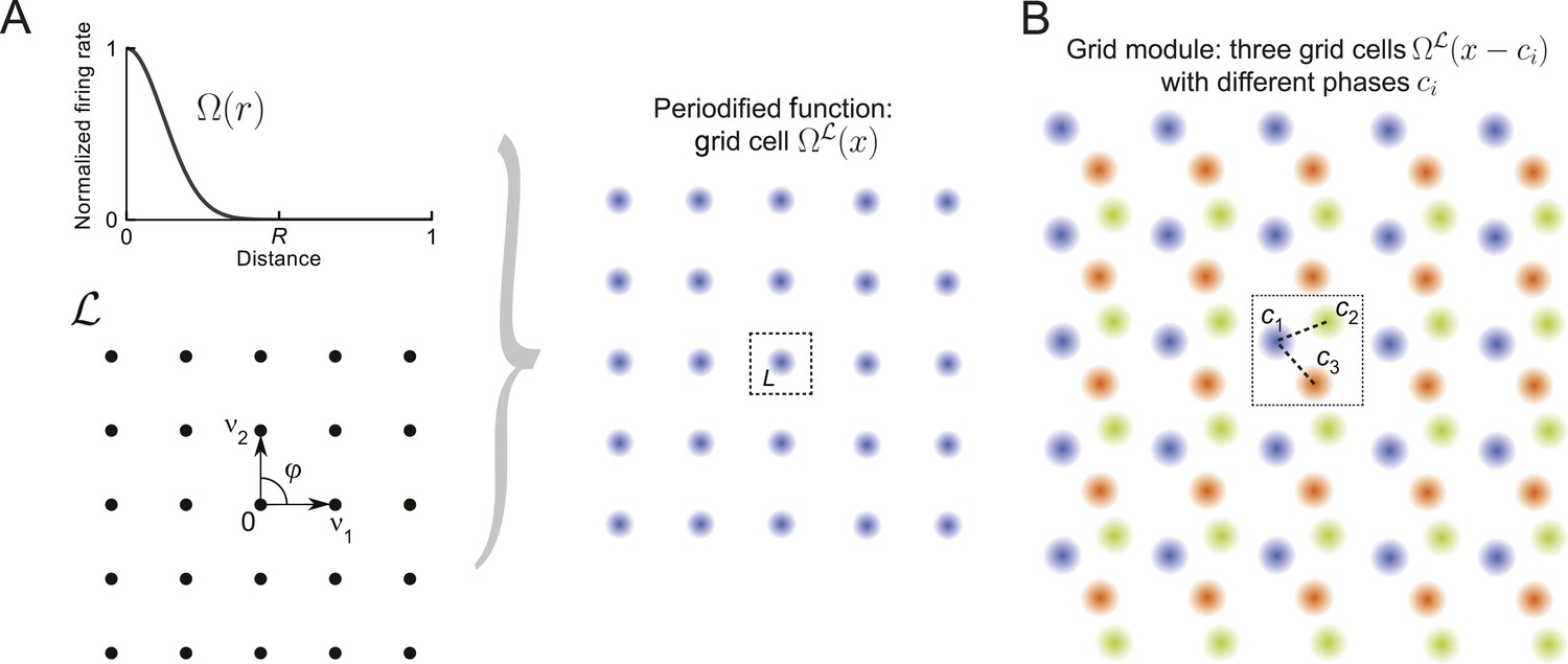
Grid cells and modules.

(A) Construction of a grid cell: Given a tuning shape Ω and a lattice $L$ , here a square lattice generated by v₁ and v₂ with φ = π/2, one periodifies Ω with respect to $L$ . One defines the value of $Ω^{L} (x)$ in the fundamental domain L as the value of Ω(r) applied to the distance from zero and then repeats this map over $ℝ^{2}$ like $L$ tiles the space. This construction can be used for lattices $L$ of arbitrary dimensions (Equation 7). (B) Grid module: The firing rates of three grid cells (orange, green, and blue) are indicated by color intensity. The cells' tuning is identical (Ω and $L$ are the same), yet they differ in their spatial phases c_i. Together, such identically tuned cells with different spatial phases define a grid module.

https://doi.org/10.7554/eLife.05979.003

Figure 2

Download asset Open asset

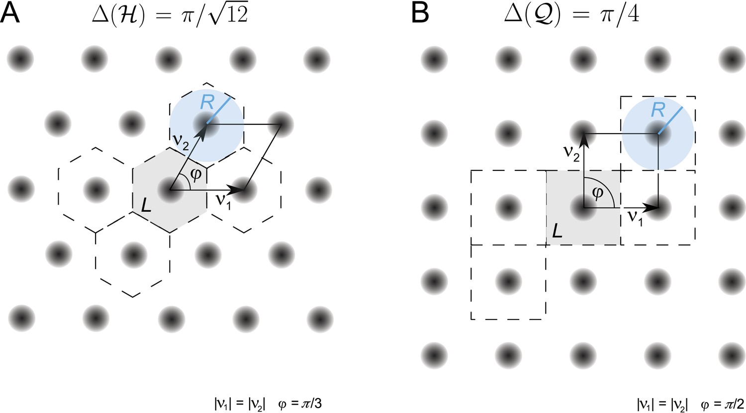
Periodified grid-cell tuning curve $Ω^{L}$ for two planar lattices, (A) the hexagonal (equilateral triangle) lattice $H$ and (B) the square lattice $Q$ , together with the basis vectors v₁ and v₂.

These are π/3 apart for the hexagonal lattice and π/2 for the square lattice. The fundamental domain, that is, the Voronoi cell around 0, is shown in gray. A few other domains that have been generated according to the lattice symmetries are marked by dashed lines. The blue disk shows the disk with maximal radius R that can be inscribed in the two fundamental domains. For equal and unitary node-to-node distances, that is, $| v_{1} | = | v_{2} | = 1$ , the maximal radius equals 1/2 for both lattices. The packing ratio Δ is $Δ (H) = π / \sqrt{12}$ for the hexagonal and $Δ (Q) = π / 4$ for the square lattice; the hexagonal lattice is approximately 15.5% denser than the square lattice.

https://doi.org/10.7554/eLife.05979.005

Figure 3 with 1 supplement

Download asset Open asset

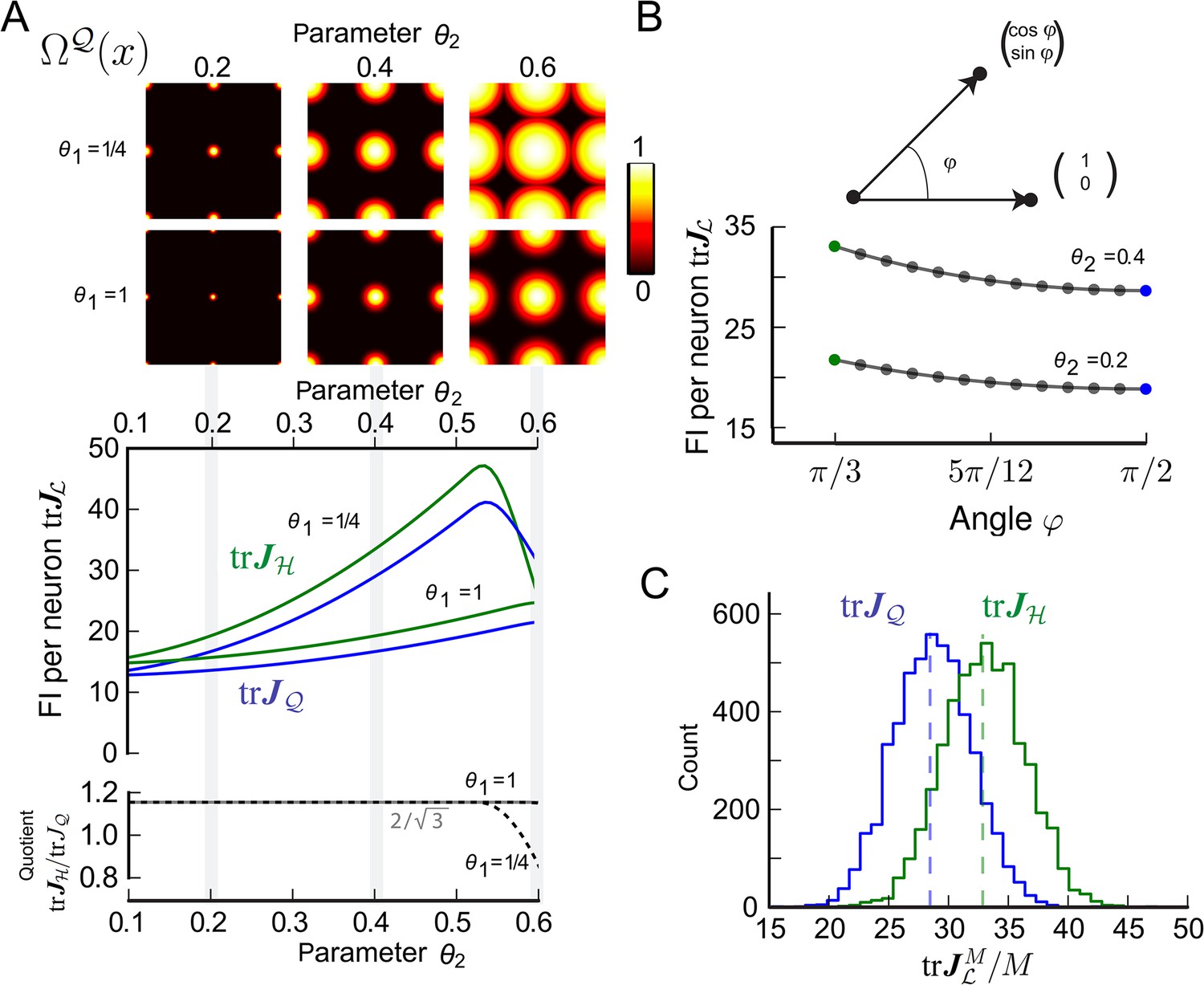
Fisher information for modules of two-dimensional grid cells.

(A) Top: Periodified bump-function Ω and square lattice $L$ , for various parameter combinations θ₁ and θ₂. Here, θ₁ modulates the decay and θ₂ the support. Middle: Average trace $tr J_{L}$ of the Fisher information (FI) for uniformly distributed grid cells $Ω^{L}$ . Hexagonal ( $H$ ) and square ( $Q$ ) lattices are considered for different θ₁ and θ₂ values. The FI of the hexagonal grid cells outperforms the quadratic grid when support is fully within the fundamental domain (θ₂ < 0.5, see main text). Bottom: Ratio $tr J_{H} / tr J_{Q}$ as a function of the tuning parameter θ₂. For θ₂ < 0.5, the hexagonal population offers 3/2 times the resolution of the square population, as predicted by the respective packing ratios. (B) Average $tr J_{L}$ for grid cells distributed uniformly in lattices generated by basis vectors separated by an angle φ (basis depicted above graph). $tr J_{L}$ behaves like 1/sin(φ) and has its maximum at π/3. (C) Distribution of 5000 realizations of $tr J_{L}^{M} / M$ at 0 for a population of M = 200 randomly distributed neurons. For both the hexagonal and square lattice, parameters are θ₁ = 1/4 and θ₂ = 0.4. The means closely match the average values in (A). However, due to the finite neuron number the FI varies strongly for different realizations, and in about 20% of the cases a square lattice module outperforms a hexagonal lattice.

https://doi.org/10.7554/eLife.05979.006

Figure 3—figure supplement 1

Download asset Open asset

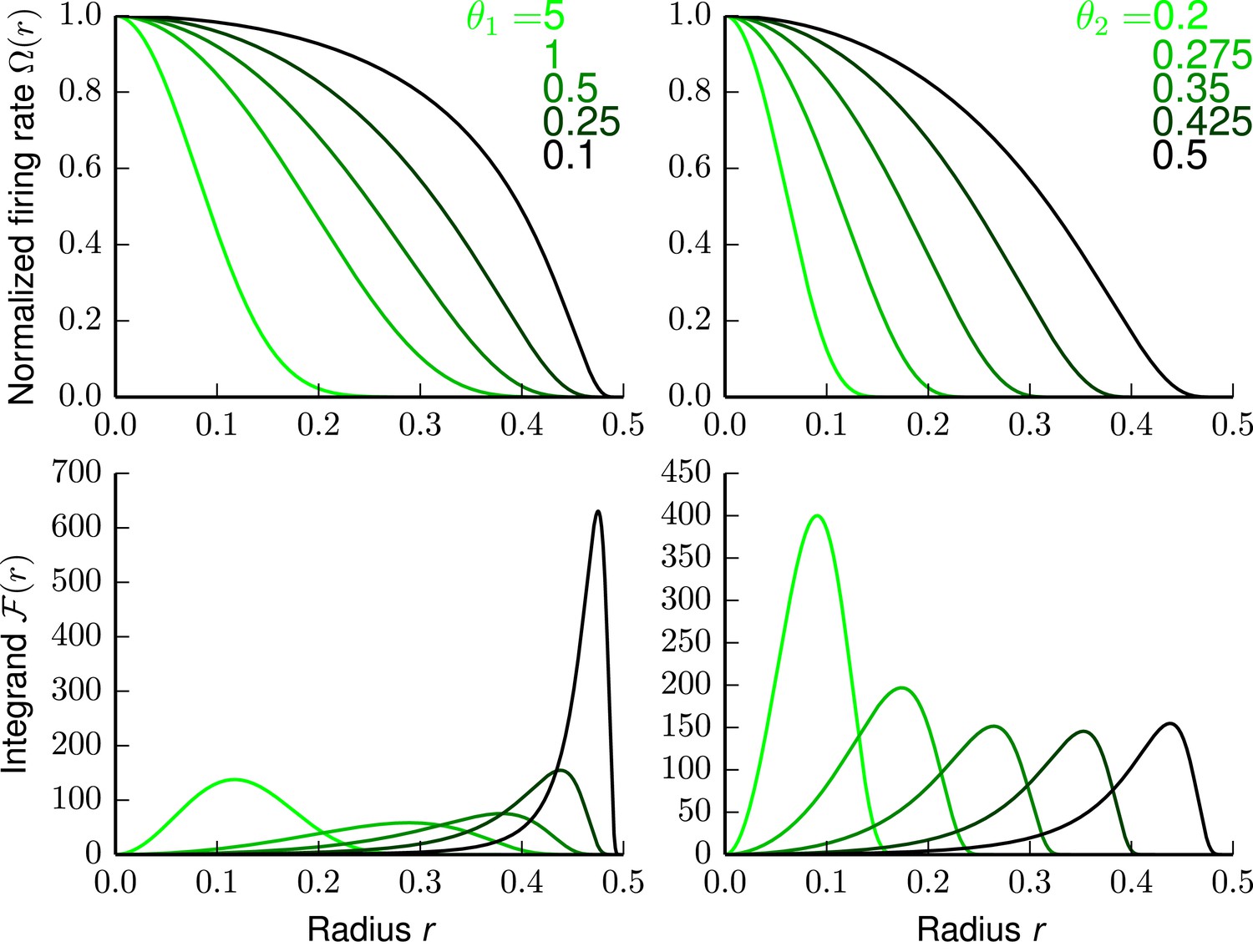
The firing rate and Fisher information of the bump tuning shape.

Upper left panel: Tuning shape Ω(r) with parameters θ₂ = 0.5 and varying θ₁. Lower left panel: Corresponding Fisher information (FI) integrand $ℱ (r)$ . Upper right panel: Tuning shape Ω(r) with parameters θ₁ = 0.25 and varying θ₂. Lower right panel: Corresponding FI integrand $ℱ (r)$ .

https://doi.org/10.7554/eLife.05979.007

Figure 4

Download asset Open asset

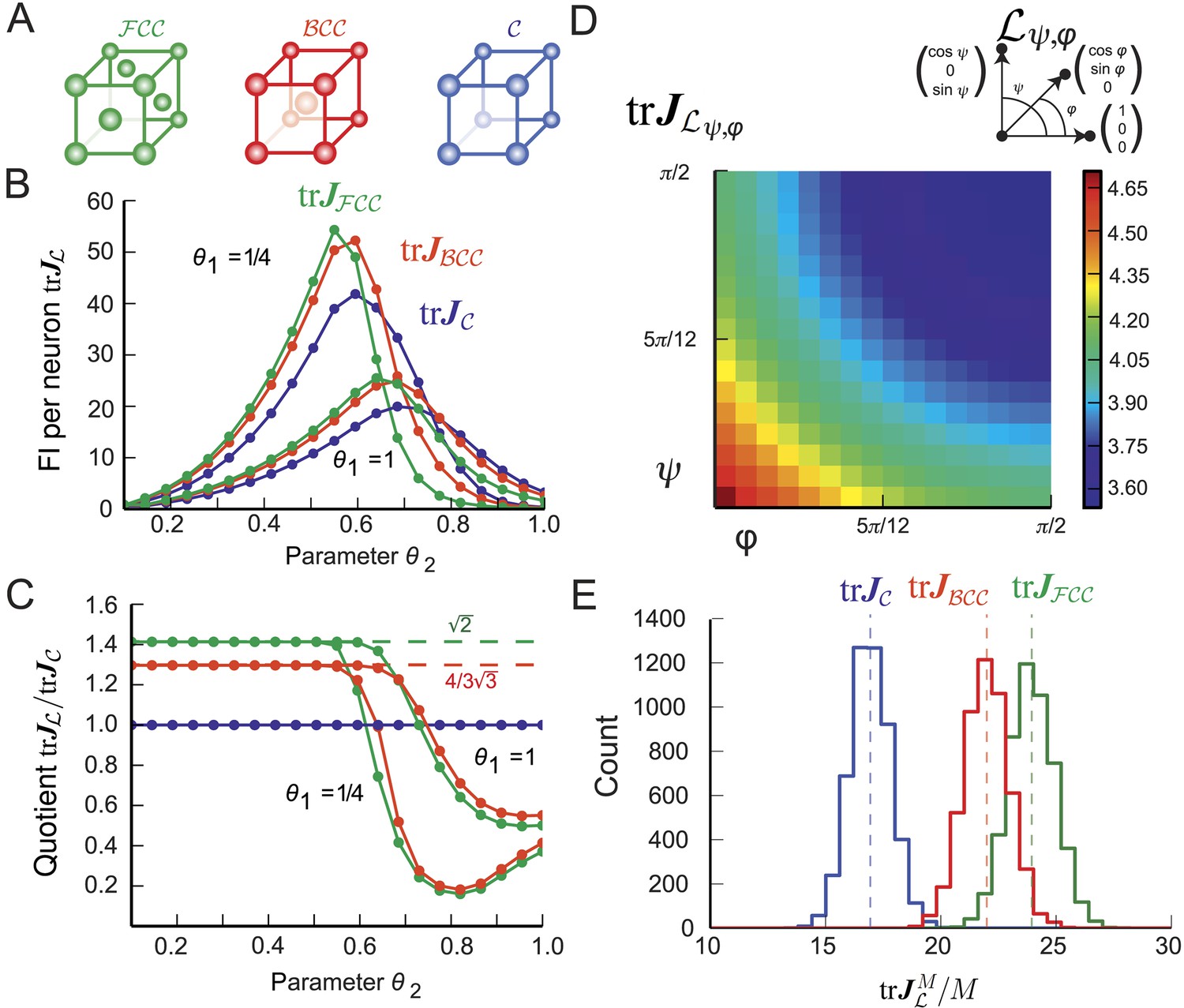
Fisher information for modules of 3D grid cells.

(A) The three lattices considered: face-centered cubic ( $F C C$ ), body-centered cubic ( $B C C$ ), and cubic ( $C$ ). (B) $tr J_{L}$ for the periodified bump-function Ω for the three lattices and various parameter combinations θ₁ and θ₂. The Fisher information (FI) of the $F C C$ grid cells outperforms the other lattices when the support is fully within the fundamental domain (θ₂ < 0.5, see main text). For larger θ₂ the best lattice depends on the relation between the Voronoi cell's boundary and the tuning curve. (C) Ratio $tr J_{L} / tr J_{C}$ as a function of θ₂ for $L \in {F C C, B C C, C}$ . For θ₂ < 0.5, the hexagonal population has 3/2 times the resolution of the square population, as predicted by the packing ratios. (D) Average $tr J_{L_{φ, ψ}}$ for uniformly distributed grid cells within a lattice $L_{φ, ψ}$ generated by basis vectors separated by angles φ and ψ (as shown above; θ₁ = θ₂ = 1/4). $tr J_{L_{φ, ψ}}$ behaves like 1/(sinφ⋅sinψ) and has its maximum for the lattice with the smallest volume. (E) Distribution of 5000 realizations of $tr J_{L}^{M} / M$ at 0 for a population of M = 200 randomly distributed neurons. Parameters: θ₁ = 1/4, θ₂ = 0.4. The means closely match the averages in (B). Due to the finite neuron number, the FI varies strongly for different realizations.

https://doi.org/10.7554/eLife.05979.008

Figure 5

Download asset Open asset

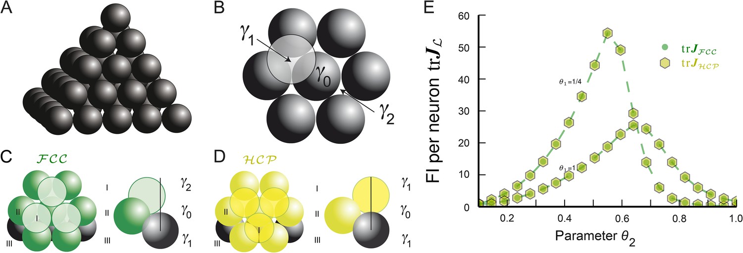
Lattice and non-lattice solutions in 3D.

(A) Stacking of spheres as in an $F C C$ lattice. In this densest lattice in 3D, each sphere touches 12 other spheres and there are four different planar hexagonal lattices through each node. (B) Over a layer of hexagonally arranged spheres centered at γ₀ (in black) one can put another hexagonal layer by starting from one of six locations, two of which are highlighted, γ₁ and γ₂. (C) If one arranges the hexagonal layers according to the sequence (…,γ₁, γ₀, γ₂,…) one obtains the $F C C$ . Note that spheres in layer I are not aligned with those in layer III. (D) Arranging the hexagonal layers following the sequence (…,γ₀, γ₁, γ₀,…) leads to the hexagonal close packing $HCP$ . Again, each sphere touches 12 other spheres. However, there is only one plane through each node for which the arrangement of the centers of the spheres is a regular hexagonal lattice. This packing has the same packing ratio as the $F C C$ , but is not a lattice. (E) $tr J_{L}$ for bump-function Ω with $L = F C C$ and $HCP$ for various parameter combinations θ₁ and θ₂; θ₁ modulates the decay and θ₂ the support. The two packings have the same packing ratio and for this tuning curve also provide identical spatial resolution. FI: Fisher information.

https://doi.org/10.7554/eLife.05979.009

Author response image 1

Download asset Open asset

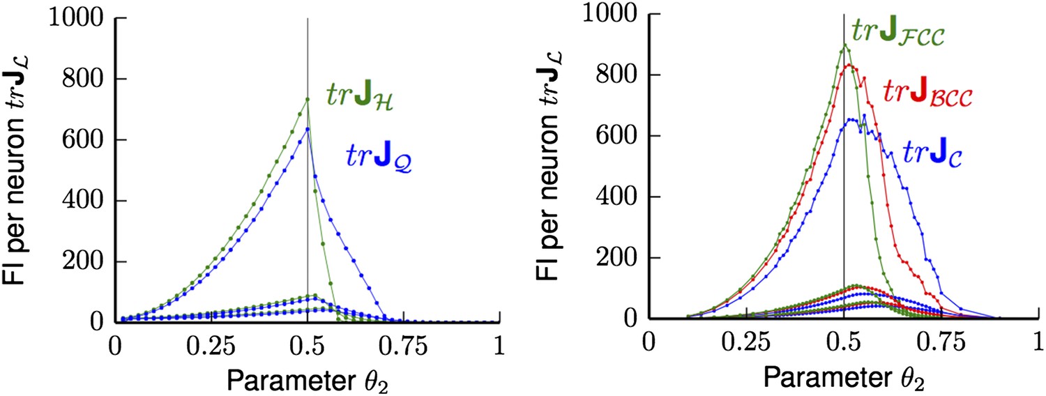
Average trace trJL of FI for uniformly distributed grid cells Ω^L for Poisson noise and bump tuning shape Ω. Left Panel: trJ_L for hexagonal (H in green) and square (Q in blue) lattices are shown for different θ₂ values, with θ₁ varying from 0.25 (lowest pair of lines), 0.1 (middle pair of lines) to 0.01 (top pair of lines). Thus, with decreasing θ₁ the FI grows and reaches the maximum at the in-radius of both lattices θ₂ = 0.5. Right panel: trJ_L for face-centered cubic (*FCC* in green), body-centered cubic (*BCC* in red) and cubic (C in blue) are shown for various θ₂ and θ₁ varying from 0.25 (lowest triple of lines), 0.1 (middle triple of lines) to 0.01 (top triple of lines). Again, the FI of the smallest θ₁ is best and reaches its peak at θ₂ = 0.5.

https://doi.org/10.7554/eLife.05979.012

Tables

Table 1

List of acronyms, variables, and terms

https://doi.org/10.7554/eLife.05979.004

D	Dimension of the stimulus space $ℝ^{D}$
FI	Fisher information, usually denoted by J (Equation 3)
$L$	Non-degenerate point lattice describing periodic structure (Equation 5)
L	Fundamental domain of $L$ , which is the Voronoi cell containing 0 (Equation 6)
Ω	Tuning shape
supp(Ω)	Support of Ω, that is, the subset where Ω does not vanish
$Ω^{L}$	Periodified tuning curve on $ℝ^{D}$ , where $L$ is a D-dimensional lattice and Ω a tuning curve. Simply referred to as a ‘grid cell’ (Equation 7)
ρ	Phase density of grid cells' phases c_i within a module $ρ (c) = {\sum^{}}_{i = 1}^{M} δ (c - c_{i})$
M	Number of phases in grid module $\int_{L} ρ = M$
$ς = (Ω, ρ, L)$	Signature defining a grid module, which is an ensemble of grid cells differing in spatial phases c_i, defined by ρ and tuning curves given by $Ω^{L}$
$det (L)$	Determinant of lattice $L$ (equal to volume of L)
B_R(0)	Subset of $ℝ^{D}$ containing all points with distance less than R from 0
$Δ (L)$	Packing ratio of a lattice, that is, the volume of the largest $B_{R} (0)$ that fits inside L divided by $det (L)$ (Equation 15)
$H$ , $Q$	Hexagonal and square planar lattice of unit node-to-node distance (Figure 2)
$F C C$ , $B C C$ , $C$	Face-centered, body-centered, and cubic lattice of unit node-to-node distance, respectively (Figure 4).
trJ	Trace of the FI, that is, the sum of diagonal elements
J_ς	Population FI of grid module with signature ς
$tr J_{L}$ , $tr J_{Q}$ , $tr J_{H}$	Trace of FI per neuron for lattice $L$ ( $Q$ and $H$ , respectively) with fixed bump-like Ω defined in Equation 26
$tr J_{L}^{M}$	Trace of FI for lattice $L$ for M randomly distributed phases in L for the same bump function