Neural tuning matches frequency-dependent time differences between the ears
- Ecole Normale Supérieure, France
- Sorbonne Universités, France
- Institut National de la Santé et de la Recherche Médicale, France
- UMR_7210, École des Neurosciences de Paris Île-de-France, Centre National de la Recherche Scientifique, France
- Albert Einstein College of Medicine, United States
- University of Leuven, Belgium
- University of Tokyo, Japan
Figures
Figure 1 with 4 supplements
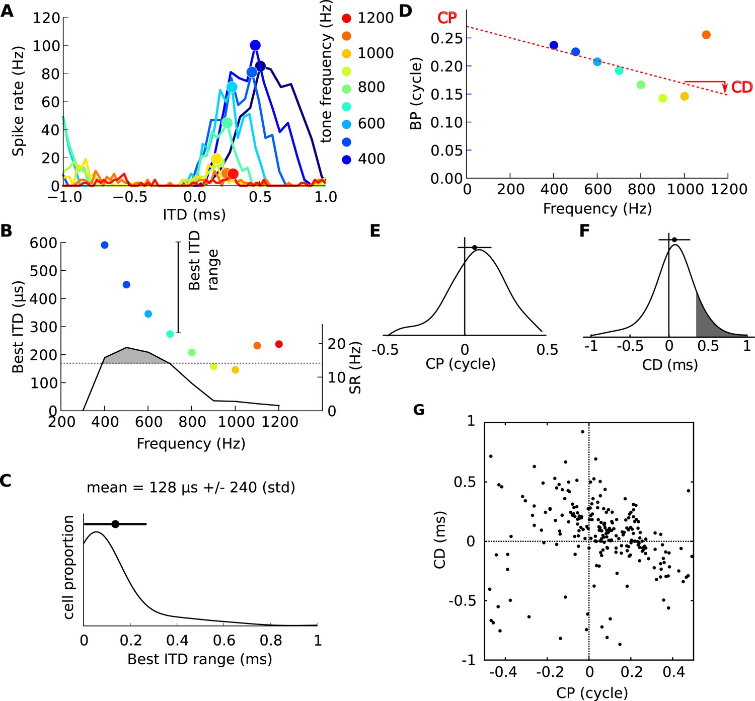
Frequency-dependence of best delays.
(A) Firing rate vs ITD for one neuron, to tones between 400 Hz (blue) and 1200 Hz (orange). (B) Best interaural time difference (ITD) (colored dots, left axis), and sync-rate (SR), (black line, right axis) vs frequency for the same cell. Data points with SR higher than 80% of the maximum value are used to calculate the range of best ITD (shaded area above dotted line). (C) Distribution of the range of best ITDs across all 186 cells. (D) Best phase (BP) vs frequency and linear regression. The characteristic phase (CP, here 0.27 cycle) is the intercept; the characteristic delay (CD, here −0.102 ms) is the slope. (E) Distribution of CP across all cells (N = 186). (F) Distribution of CD. (G) CD vs CP across all cells.
Figure 1—figure supplement 1
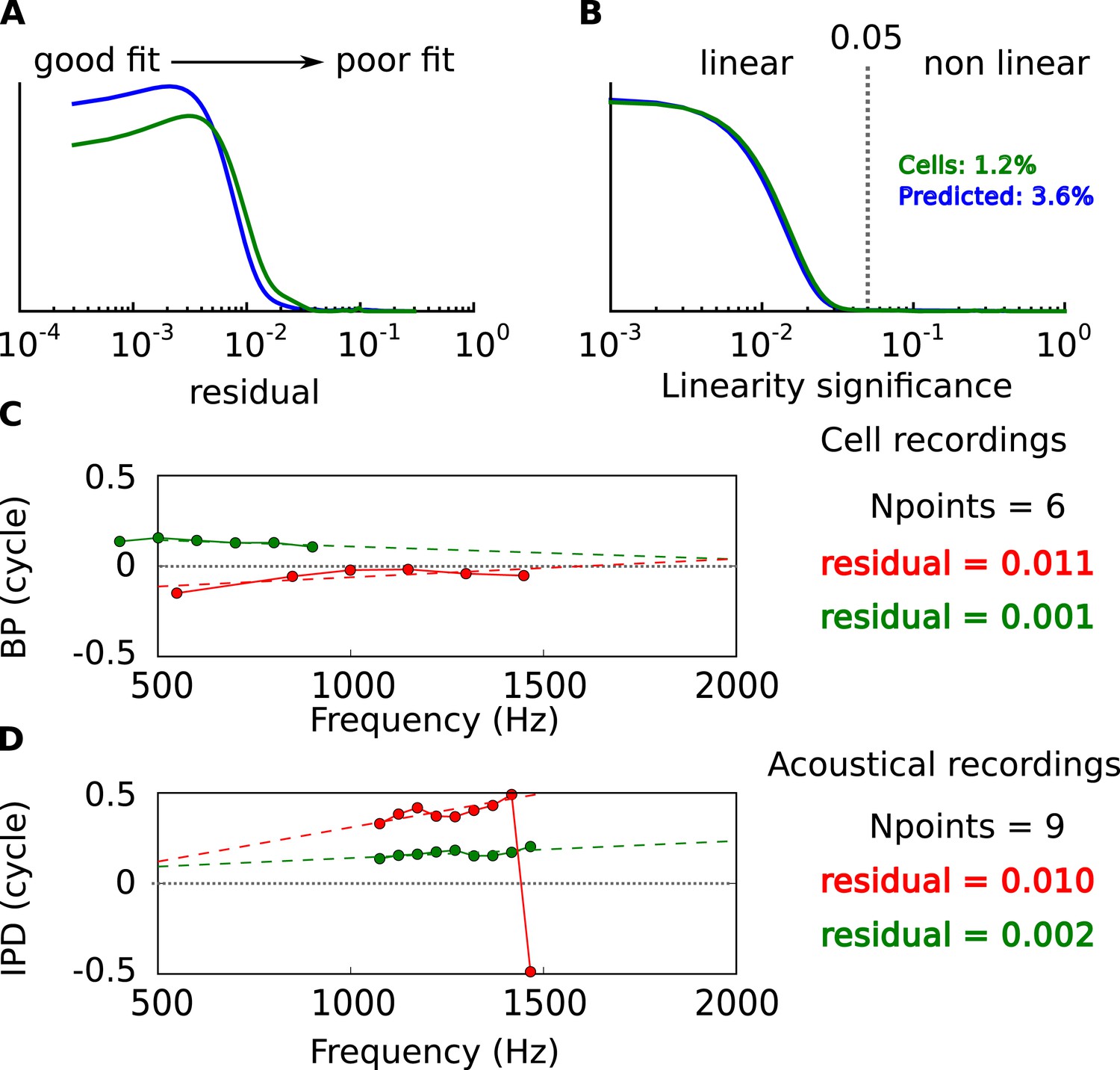
Linearity of BP vs frequency curves.
(A) Distribution of residual error in linear fits of BP vs frequency in cells (green) and in acoustical predictions (blue). (B) Statistical significance of linear fits. Cells are selected for further analysis when p < 0.05. Percentage: proportion of nonlinear cells and prediction from the acoustics. (C) BP vs frequency and linear regressions for two cells with the same number of frequency points and different residual errors. (D) Same as C, for acoustical recordings.
Figure 1—figure supplement 2
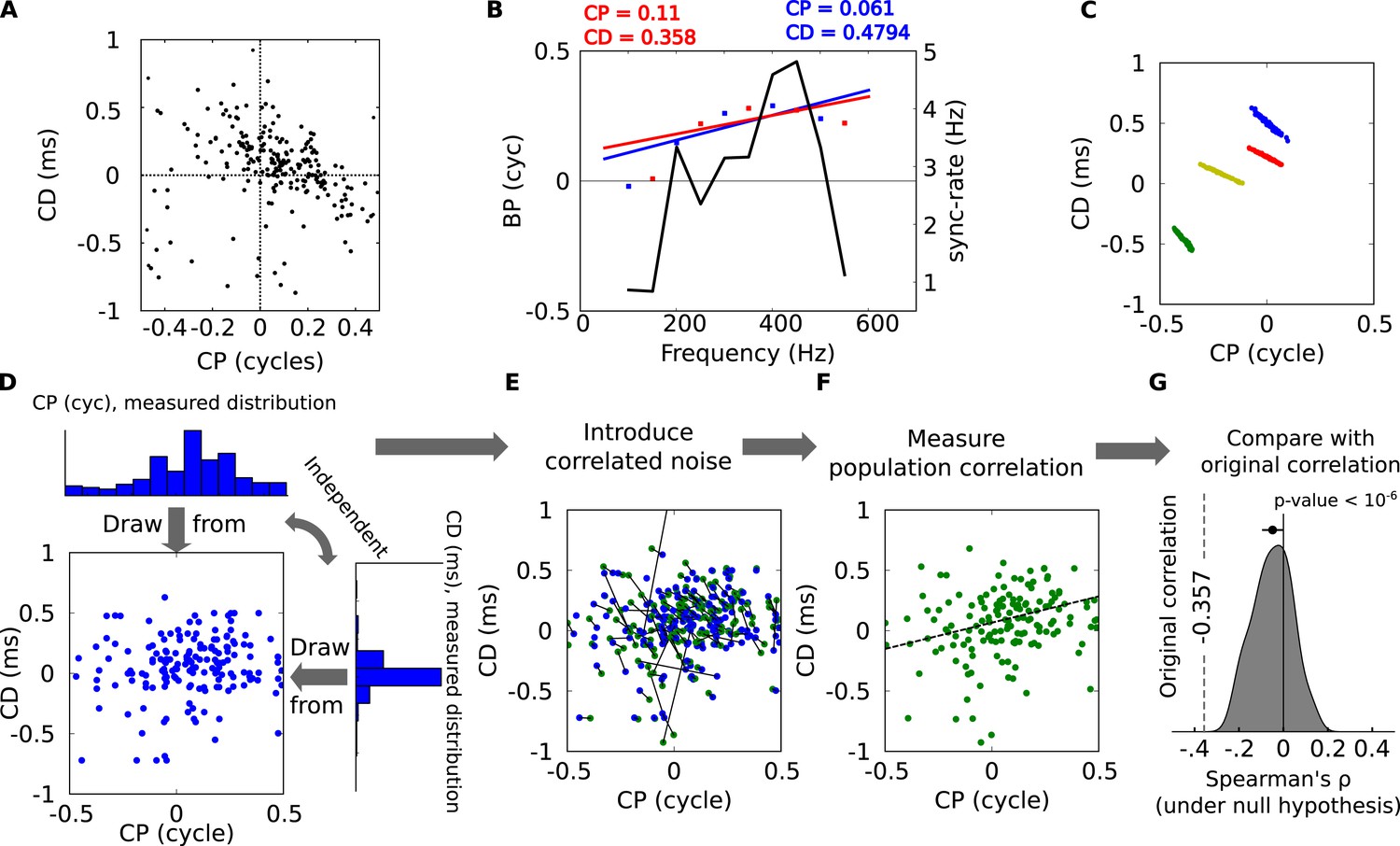
Statistical significance of CP-CD correlation.
(A) Characteristic delay (CD) vs characteristic phase (CP) for all cells. Spearman's rank correlation ρ is −0.357. (B) Illustration of spurious correlations due to noise. Two subsets of BP vs frequency data points (red and blue dots) from the same neuron are fitted with lines: intercept (CP) and slope (CD) are inversely correlated. The solid curve shows the SR (see ‘Materials and methods’). (C) Linear regression performed on bootstrap samples for 4 cells: CD and CP are inversely correlated for each cell, but positively correlated overall. (D–G) Statistical test of CP-CD correlation. (D) Data points are generated at random under the hypothesis that CP and CD are independent, using the distributions measured in cells. (E) Correlated noise is added to each (CP, CD) point shown in D, with the correlated noise distributions previously measured as in panel C. Each new point is shown in green, connected by a line to the original point (blue). (F) Correlation is measured across all green points of E (dashed: linear regression). The procedure D–F is reiterated many times with new sets of random samples. (G) The distribution of Spearman's ρ in the generated data points has a small negative bias, much smaller than in the original data points (dashed, p < 10−6).
Figure 1—figure supplement 3
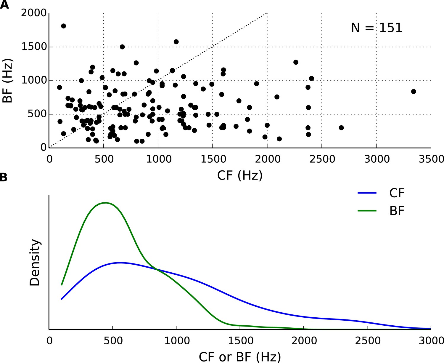
Best frequency (BF) and characteristic frequency (CF) of recorded cells.
(A) Each cell's BF plotted against the CF. (B) Distributions of BF and CF in the population of cells.
Figure 1—figure supplement 4
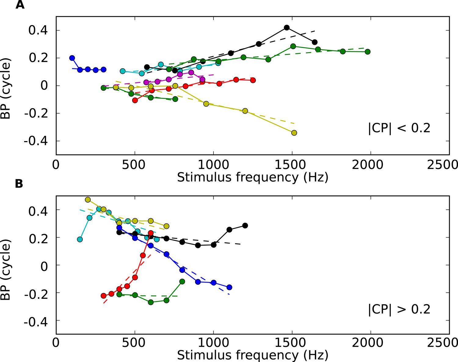
BP vs tone frequency for 13 sample cells.
(A) BP vs frequency for cells with low CP values (below 0.2 cycles), with regression lines (dotted). (B) BP vs frequency for cells with higher CP values.
Figure 2 with 1 supplement
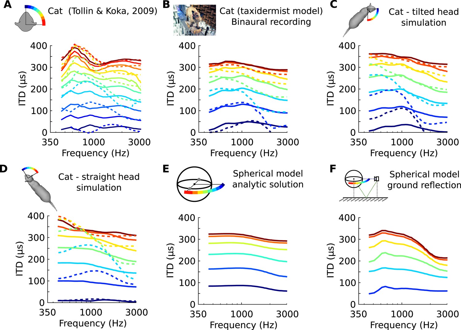
Frequency-dependence of ITD in several acoustical datasets.
(A) ITD vs frequency for sound directions on the horizontal plane (azimuth 15–90°, spaced by 15°), measured in a live cat and previously reported (Roth et al., 1980). (B) Acoustical measurements on a taxidermist model of a cat in a large anechoic room (same azimuths). Dashed curves show symmetric positions for sources to the back of the animal. Note that the head is tilted to the right; azimuths are relative to the head (not the body). (C) Numerical calculation of ITDs by boundary element method (BEM) simulation on a 3D model of the same cat as B (grey shape), obtained from photographs. (D) Same as C, but with a straightened head. (E) Analytical calculation of ITDs for a spherical rigid head. (F) Same as E, but with an additional reflection from the ground. Head and source are placed 1.7 meter from each other and 20 cm above the ground.
Figure 2—figure supplement 1
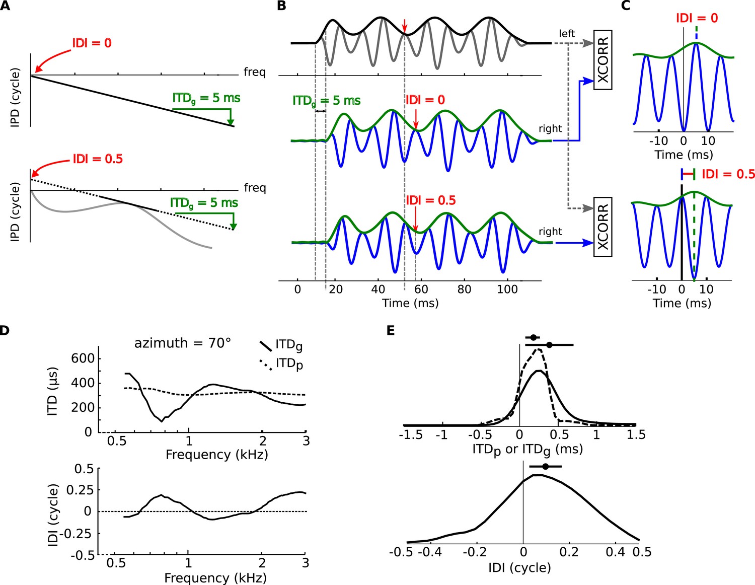
Envelope and fine-structure ITDs.
(A) Top: linear IPD curve (constant ITD) with ITDg = 5 ms (group ITD, see ‘Materials and methods’). Bottom: If the IPD is nonlinear (gray curve), then it can be locally approximated with an affine function (black plain and dotted line). This introduces a non-zero IDI (Interaural Diffraction Index, see ‘Materials and methods’). (B) an amplitude modulated tone (top panel, black: envelope, gray: signal) models the left monaural signal. The right signal is passed through model head-related transfer functions (HRTFs) with either ITDg = 5 ms, and IDI = 0 cycles (middle panel) or ITDg = 5 ms and IDI = 0.5 cycles (bottom panel). The right signal (blue: signal, green: envelope) is delayed by the amount of the ITDg, while the fine structure of the signal undergoes an additional phase shift equal to the IDI (see text). (C) interaural cross-correlation functions in the two cases IDI = 0 (top) and IDI = 0.5 (bottom). The envelope peak (green segment) is unaffected by the IDI, while the fine structure peak (blue segment) is shifted by an amount (in phase) equal to the IDI. (D) ITDp (phase ITD, see ‘Materials and methods’) and ITDg for one position of the cat HRTFs (top panel), IDI for the same position (bottom panel) as a function of frequency. (E) Top: Distribution of ITDp (dashed line) and ITDg (solid line) in the cat over all positions and frequencies. Bottom: Distribution of IDI.
Figure 3 with 1 supplement
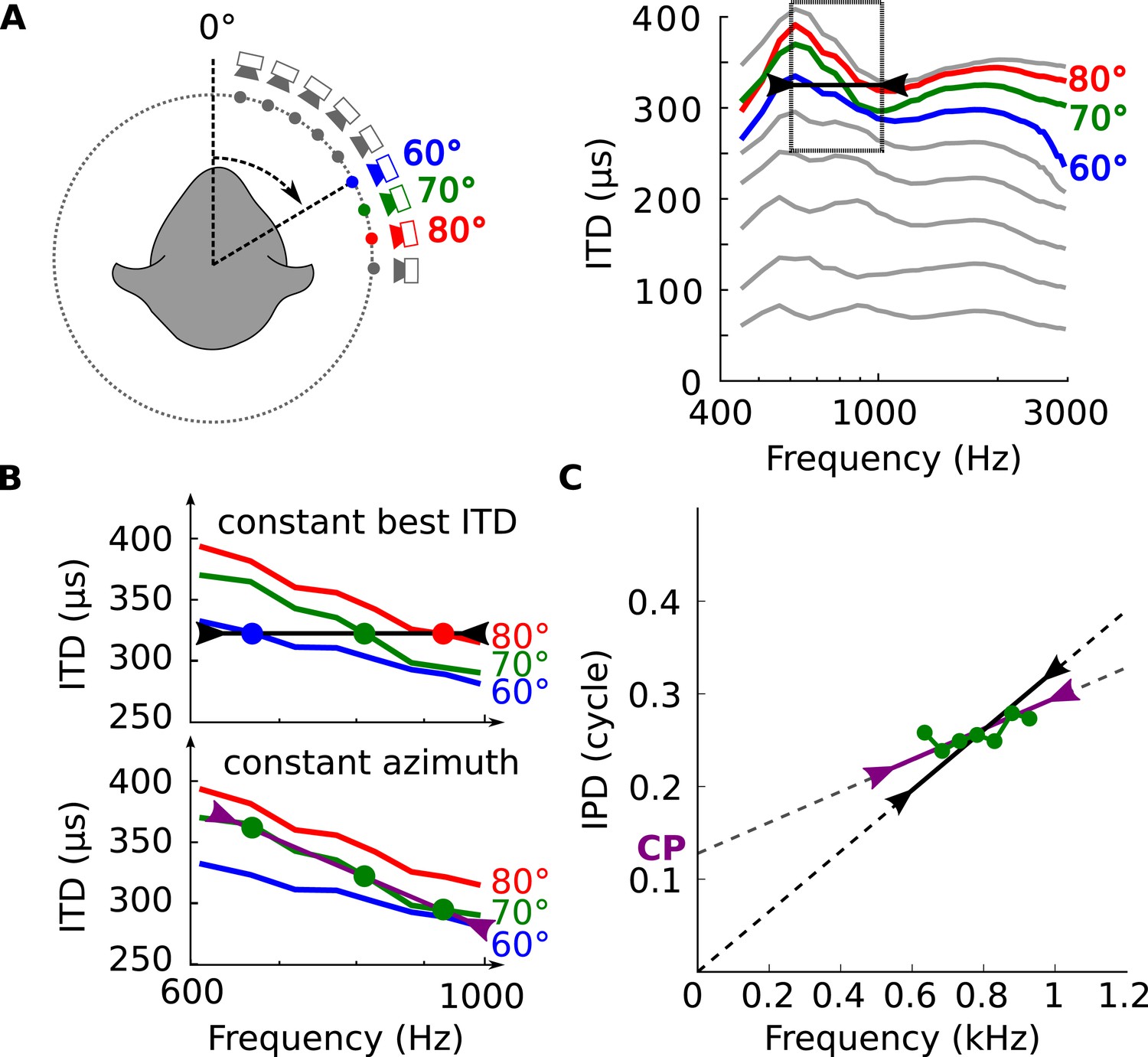
Tuning to frequency-dependent ITDs.
(A) Left, head-related transfer functions (HRTFs) are measured binaurally for different speaker positions. Right, ITD vs frequency in cat at 60, 70 and 80° on the horizontal plane. (B) A neuron for which best ITD is fixed across frequency (top, black line) is tuned to different azimuths depending on frequency, while a neuron with fixed azimuth tuning has a frequency-dependent best ITD (bottom, purple line). (C) IPD vs frequency at 70° over a 300 Hz window around 800 Hz (green curve and circles). The black segment represents an ITD of 325 μs that is fixed across frequency, equal to the ITD at 800 Hz. The purple segment represents the best linear approximation of IPD around that frequency (intercept 0.12 cycle, slope 167 μs).
Figure 3—figure supplement 1
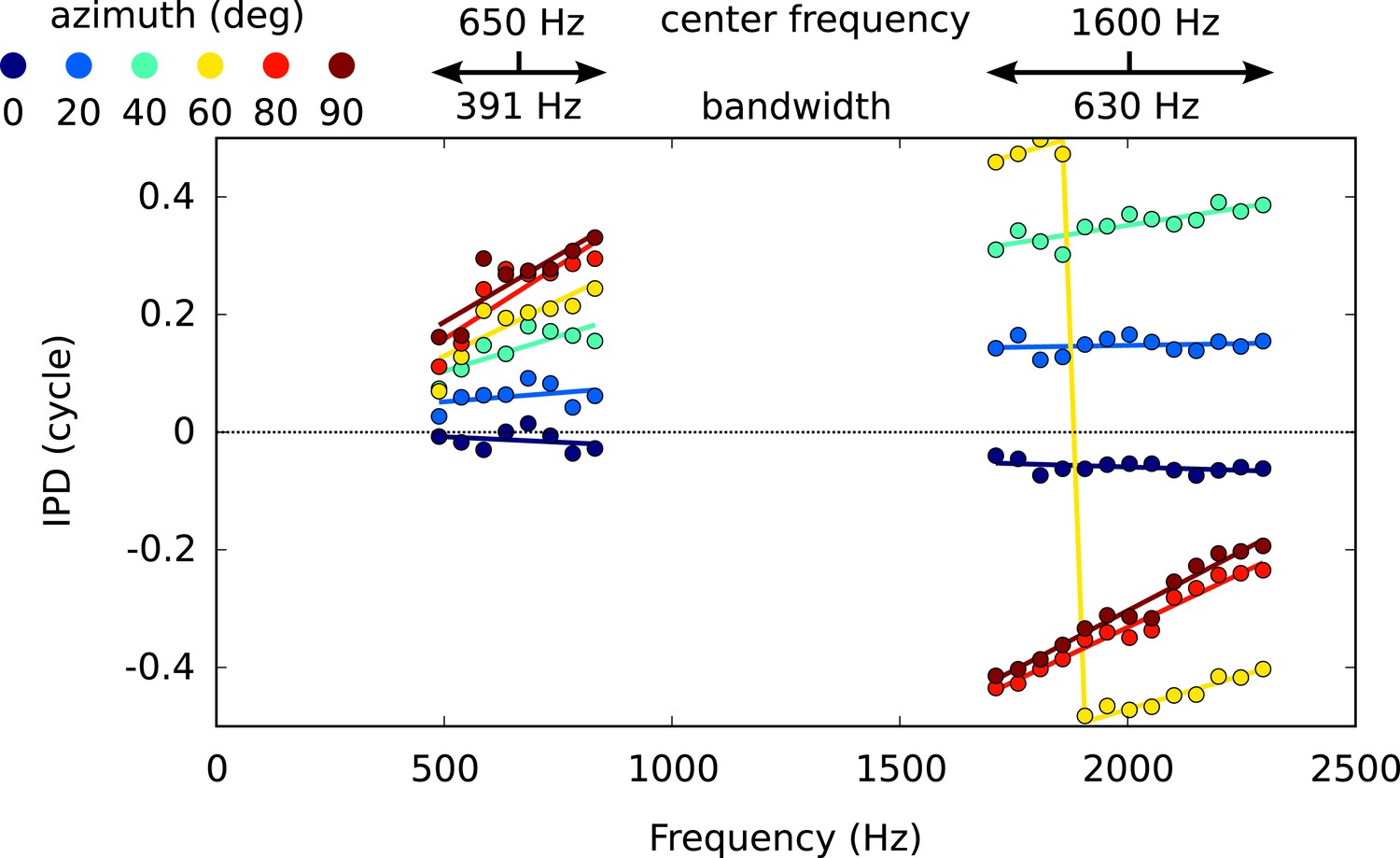
IPD vs frequency for six different directions, around 650 Hz and 1600 Hz, with circular-linear fits.
https://doi.org/10.7554/eLife.06072.011
Figure 4 with 3 supplements

Acoustical analysis.
(A) Distribution of CP in the cells (green) and in the acoustics based on acoustical measurements (blue). Error bars represent the mean ± STD/2, and percentages the proportion of positive/negative values. (B) Distribution of CD in cells (green) and in acoustics (blue). (C) CD vs CP in the acoustics.
Figure 4—figure supplement 1
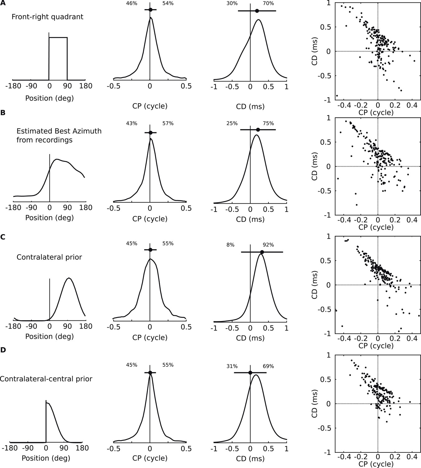
Acoustical predictions of CD and CP distributions for various prior spatial distributions.
First column: distribution of preferred positions. Second and third columns: prediction of CP and CD distributions (numbers are proportions of positive and negative values). Fourth column: joint CP-CD distributions (200 sample cells drawn at random). (A) Uniform distribution of preferred positions in the 0–90° quadrant. (B) Distribution of preferred positions inferred from cell recordings (best fits to HRTFs, see ‘Materials and methods’). (C) Bias for positions near 90°. (D) Bias for positions near the center.
Figure 4—figure supplement 2
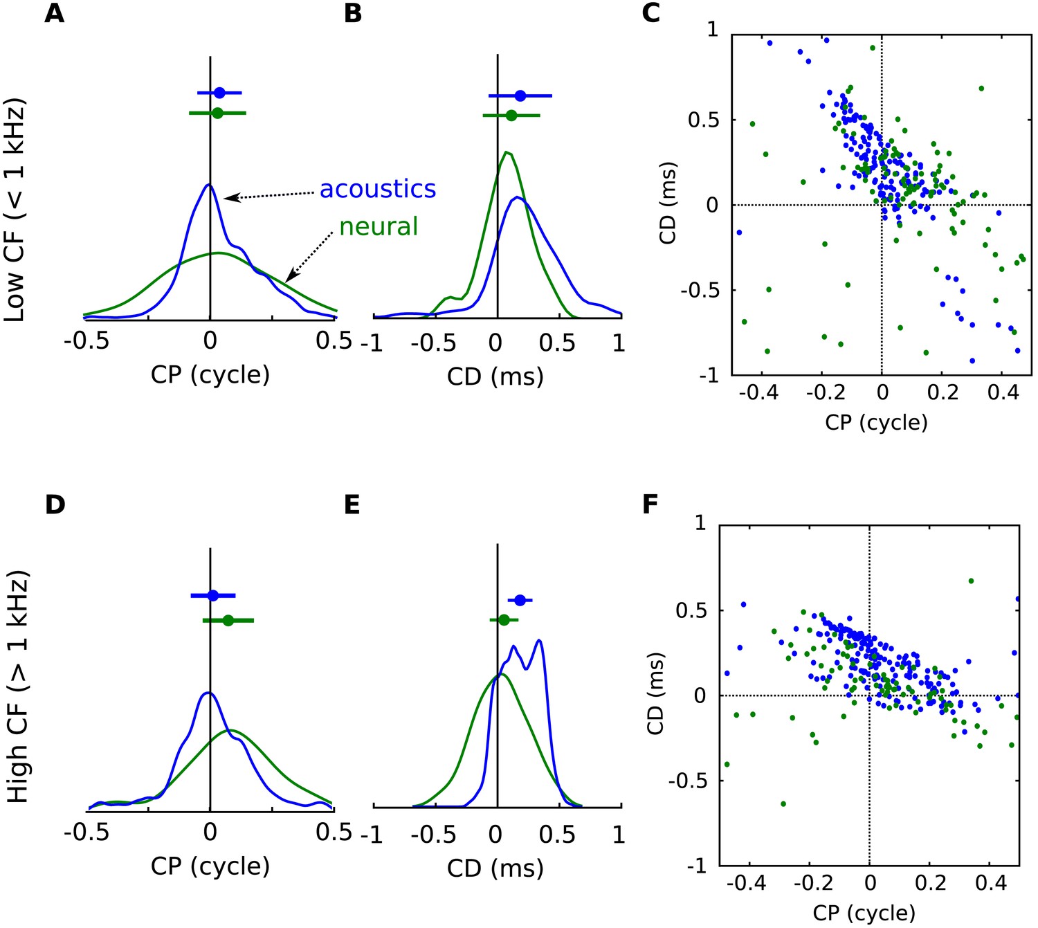
Acoustical predictions of CD and CP distributions in low and high frequency regions.
(A) Distribution of CP in the cells (green) and in the acoustics based on acoustical measurements (blue), for frequency bands below 1 kHz. (B) Distribution of CD in cells (green) and in acoustics (blue), for frequency bands below 1 kHz. (C) CD vs CP in the acoustics, for frequency bands below 1 kHz. (D–F) same as A–C for frequency bands above 1 kHz.
Figure 4—figure supplement 3
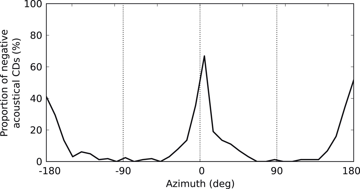
Negative acoustical CDs.
Proportion of negative (i.e., ispilateral-leading) CDs in the cat HRTFs as a function of azimuth.
Figure 5
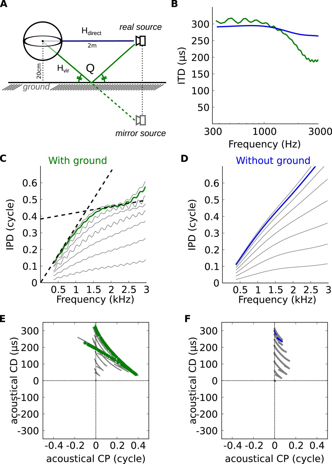
Theoretical explanation of inverse CP-CD relationship.
(A) A spherical head model with a ground reflection. (B) ITD vs frequency in the spherical model for a source at 70°, with (green) and without (blue) ground reflection. (C, D) IPD vs frequency for the same position as in B (green and blue) and for other positions between 0 and 90° (light gray curves). (E, F) Predicted CD vs CP for the two cases.
Figure 6
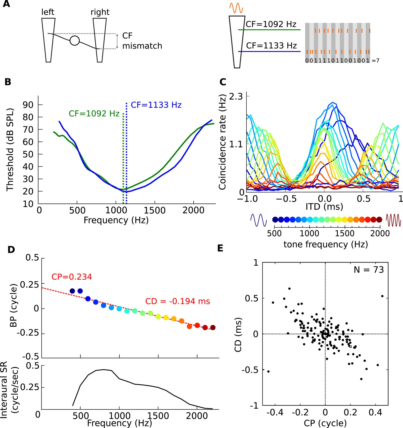
Mechanism for frequency-dependent neural tuning.
(A) Schematics of the coincidence analysis. The left schematic illustrates the concept of cochlear disparities. The trapezoids schematize the cochlear basilar membrane. A left and right fiber originate from a different cochlear place and converge on a binaural neuron. The right schematic illustrates the counting of coincidences between spike trains from two fibers in response to a single tone. Due to the cochlear traveling wave, the spike trains of the more apical (green) fiber are expected to be delayed in time and lagged in phase relative to the more basal (blue) fiber. (B) Threshold tuning curves of the two example fibers. (C) Pseudobinaural tuning curves: Coincidence counts as a function of ITD for a pair of fibers for different tone frequencies. Each curve is color coded with the frequency of the stimulus, scale is presented below the plot. (D) BP as a function of frequency for the same nerve pair as C. (E) CD vs CP over a population of coincidence detectors receiving inputs from cat auditory nerve fibers with mismatched CF (<0.1 octave; CF < 3.3 kHz).
Figure 7
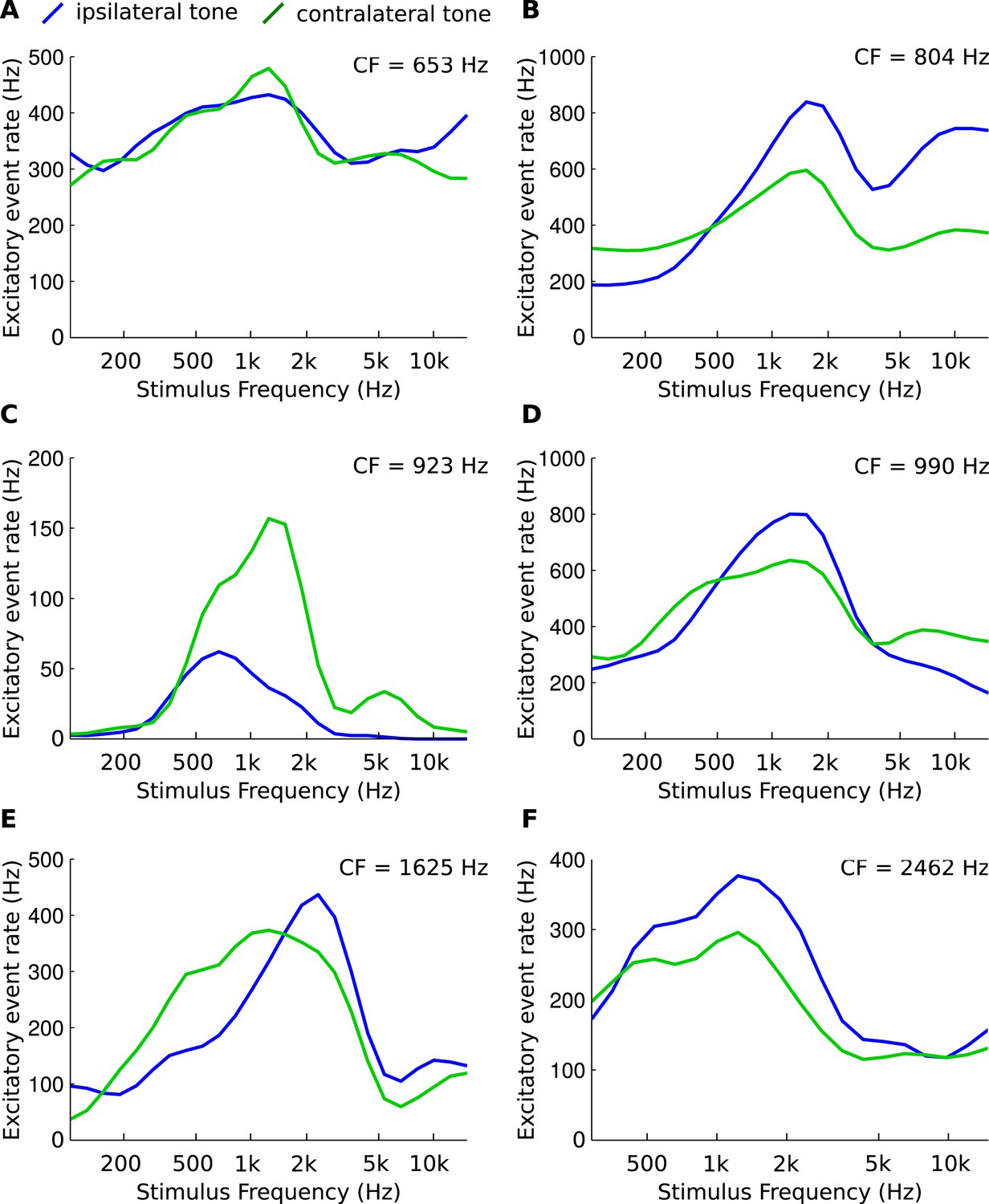
Asymmetries in frequency tuning in the excitatory inputs to the gerbil medial superior olive (MSO).
(A–F) Rate of excitatory presynaptic events (EPSPs) in 6 MSO cells, with different CF, in response to tones as a function of frequency. Stimuli are presented ipsilaterally (blue function) or contralaterally (green function). Only EPSPs ≥ the median EPSP amplitude are included. Functions were smoothed using a 3-point running average.
Figure 8
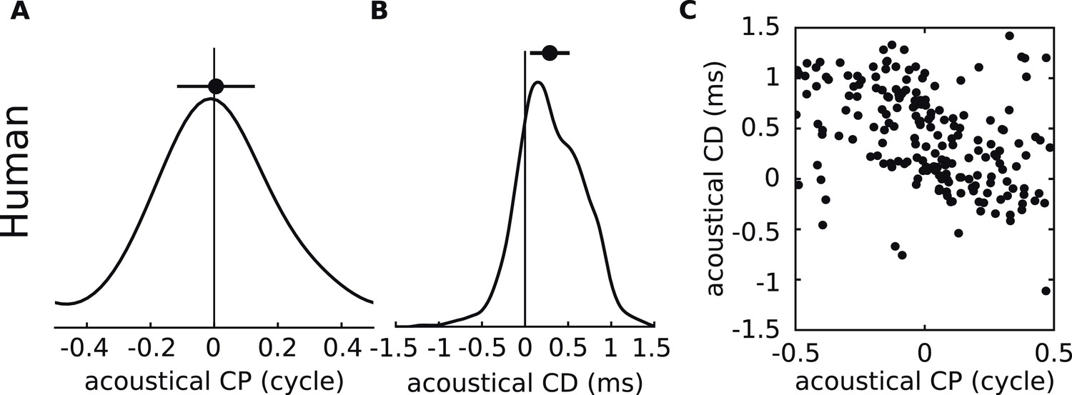
Acoustical analysis of human.
(A–C) Predictions using human HRTFs (IRCAM LISTEN HRTF database) for the distributions of acoustical CP (A), CD (B) and 200 sample points from the joint CP-CD distribution (C) over a 100–1500 Hz frequency range.
Download links
A two-part list of links to download the article, or parts of the article, in various formats.
Downloads (link to download the article as PDF)
Open citations (links to open the citations from this article in various online reference manager services)
Cite this article (links to download the citations from this article in formats compatible with various reference manager tools)
Neural tuning matches frequency-dependent time differences between the ears
eLife 4:e06072.
https://doi.org/10.7554/eLife.06072


