Attention stabilizes the shared gain of V4 populations
- Howard Hughes Medical Institute, New York University, United States
- University of Pittsburgh, United States
Figures
Figure 1 with 2 supplements
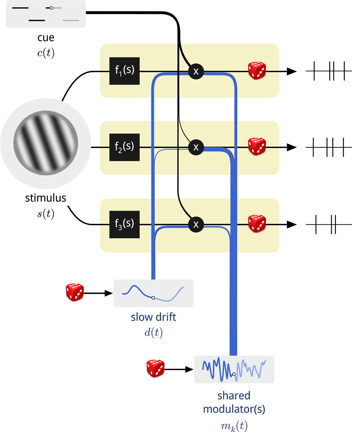
Diagram of the modulated population model.
Shown are three neurons (yellow boxes), each with a firing rate that is a function of the stimulus multiplied by three time-varying gain signals: the binary attentional cue; a slow global drift; and a set of shared modulators. The influence of each of these signals on each neuron is determined by a coupling weight, indicated by the thickness of the blue and black lines. Only one shared modulator is shown in this schematic, but the model allows for more, each with its own coupling weights. The spike counts of each neuron are conditionally Poisson, given the firing rate.
Figure 1—figure supplement 1
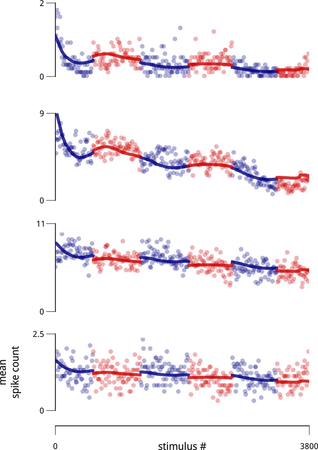
Example slow drifts in spike counts of four simultaneously-recorded units (two from each hemisphere), taken from a recorded population of 77 units.
Each point is the average spike count observed over ten consecutive stimulus presentations. The blocked structure of the task (i.e. the alternating cue directions) is indicated with alternating colors. Thick lines indicate the portion of model-estimated firing rate due to the combination of stimulus drive, cue, and the slow drift signal (without the shared modulators).
Figure 1—figure supplement 2
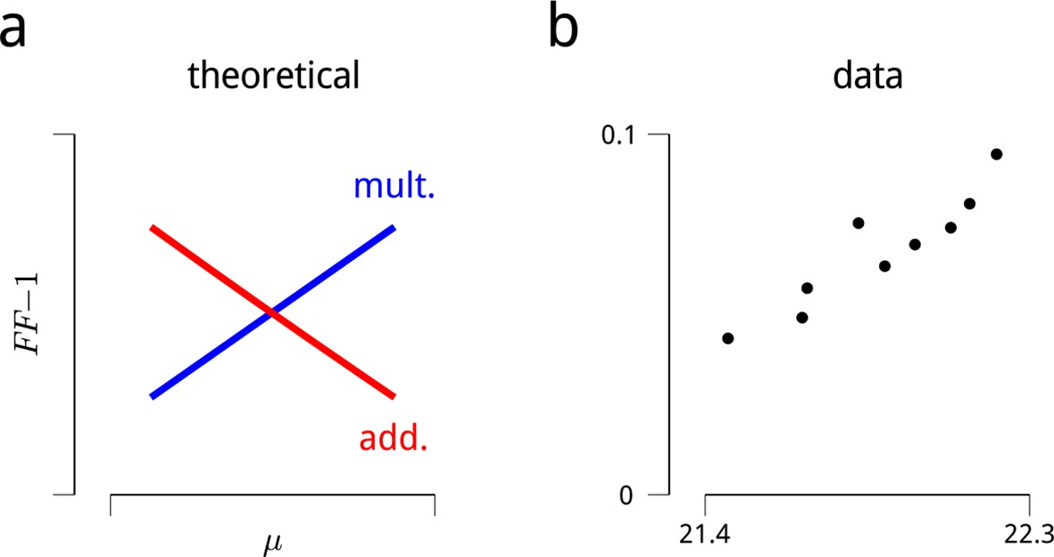
Signatures of modulatory (multiplicative) effects in the neural responses.
The shared modulator model is based on the assumption that the stimulus-driven firing rates of sensory neurons are modulated (multiplied) by a set of additional inputs. Evidence for fluctuating modulation of sensory responses was recently provided in (Goris et al., 2014). The statistical argument that these inputs are multiplicative (rather than additive) is based on a consideration of their effects as a function of firing rate: multiplicative noise has its greatest effects on response variance (and covariance) for stimuli evoking high firing rates, while additive noise has its greatest effects on response variance (and covariance) for stimuli evoking low firing rates. This is difficult to assess in the context of the V4 attentional dataset, since the standard stimuli were all identical, and responses to the targets were often interrupted by saccades. Restricting the analysis to target responses that were not interrupted is possible, but such conditioning on a behavioral state (and likely a modulator state) would complicate any interpretation. There was, however, some variability in evoked firing rates arising from adaptation. Many neurons showed a trend of slightly decreasing response to the sequence of standard stimuli, with an average total decrease of ∼5% in firing rate over the ten presentations after the first. This decrease was sufficiently small that including it in the analysis of the main text only marginally improved predictive log-likelihoods (as in Figure 2a), and did not qualitatively change any of the main results or conclusions. These small changes in firing rate over the stimulus sequence were nevertheless sufficient to examine the hypothesis that neural response variance was due a multiplicative noise source. Following the logic of (Goris et al., 2014), if we assume a multiplicative noise source with variance σ2, the Fano factor (variance divided by the mean) should increase with firing rate, μ:
On the other hand, for an additive noise source of variance σ2, the Fano factor should decrease with firing rate:
These expected trends are illustrated in panel (a). Panel (b) shows the mean value of these quantities, estimated for the cue-towards condition across all cells. The data are clearly consistent with a multiplicative noise source. A similar trend is observed in the cue-away condition, albeit with an overall lower mean rate, and higher Fano factor. This analysis assumes that the noise source has constant variance across stimulus conditions. There were some small, non-monotonic changes in the estimated shared modulators’ variance over the stimulus sequence. Factoring these in does not change the direction of the predictions or the data shown here. A similar analysis can be performed on pairwise response statistics (as stimuli evoke higher mean rates, a multiplicative model predicts correlations will increase, while an additive model predicts correlations will decrease). But these predictions prove more sensitive to the assumption of stability in σ2, so we omit them here.
Figure 2 with 4 supplements
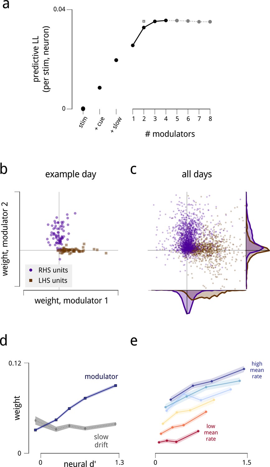
The fitted model explains the observed spiking responses, with estimated modulators that are both anatomically and functionally targeted.
(a) Performance comparison of various submodels, measured as log-likelihood (LL) of predictions on held-out data. Values are expressed relative to performance of a stimulus-drive-only model (leftmost point), and increase as each model component (cue, slow drift, and different numbers of shared modulators) is incorporated. The grey square shows the predictive LL for a two-modulator model, with each modulator constrained to affect only one hemisphere (i.e. with coupling weights set to zero for neurons in the other hemisphere). This restricted model is used for all results from Figure 2d onwards, excepting the fine temporal analysis of Figure 6c. (b) Modulators are anatomically selective. Inferred coupling weights for a two-modulator model, fit to a population of units recorded on one day. Each point corresponds to one unit. As the model does not uniquely define the coordinate system (i.e. there is an equivalent model for any rotation of the coordinate system), we align the mean weight for LHS units to lie along the positive x-axis (see Materials and methods). (c) Distribution of inferred coupling weights aggregated over all recording days indicates that each shared modulator provides input primarily to cells in one hemisphere. (d) Hemispheric modulators are functionally selective. Units which are better able to discriminate standard and target stimuli in the cue-away condition have larger coupling weights (blue line). Discriminability is estimated as the difference in mean spike count between standard and target stimuli, divided by the square root of their average variance (d′). Values are averaged over units recorded on all days, subdivided into five groups based on their coupling weights. Shaded area denotes ±1 standard error. Pearson correlation over all units is r = 0.42. This relationship is not seen for the weights that couple neurons to the slow global drift signal (gray line, Pearson correlation r = 0.00). The relationship between d′ and cue weight is significant, but weaker than for modulator weight (r = 0.24); this is not shown here as the cue weights are differently scaled. (e) Same as in (d), but with units subdivided into subgroups according to mean firing rate. Each line represents a subpopulation of ∼500 units with similar firing rates (from red to blue: 0–7; 7–12; 12–17; 17–25; 25–35; 35–107 spikes/s). Within each group, the Pearson correlations between d′ and coupling weight are between 0.2–0.3, but the correlations between mean rate and coupling weight are weak or negligible.
Figure 2—figure supplement 1
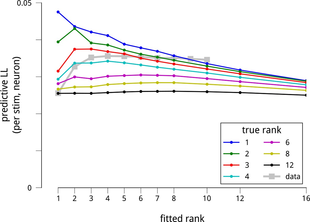
The dataset is sufficient to support the estimation of up to 8 shared modulators.
To test whether the number of recovered modulators is limited by insufficiency of the dataset, we simulated data from model neural populations that were under the influence of different numbers of modulators. All simulated datasets were matched in size to the physiological data, and simulated shared gain fluctuations were adjusted in amplitude to produce the same pairwise spike count statistics as the actual data. We then fit the model to these synthetic datasets, and measured how well the model fits recovered the true modulatory structure. More specifically, we extracted default model parameters by fitting each neural population: the stimulus-driven mean firing rates F, the cue-dependent gains C, and the slow global drifts D. Then, for a given number of simulated modulators K (from 1 to 12), we sampled a (T × K) matrix of time-varying modulator values (each value i.i.d. Gaussian), and a (K × N) matrix of random weights (each weight i.i.d. Gaussian), producing a net modulator matrix M as the matrix product of these two. We then sampled spike counts Y from the generative model, . For each population and K, we chose the scaling parameter λ such that the median noise correlation between the simulated neurons matched the median noise correlation between the actual neurons. We next fitted the models to these simulated datasets to see how well they recovered the underlying structure. As for the actual data (Figure 2), we evaluated the model fits via the predictive log-likelihood on held-out data. Each colored line shows the predictive LLs of the fitted models for a given “ground truth” number of modulators. In comparison, the grey squares show the model performance for the actual data. There are two important patterns here. First, for simulated models containing up to 8 modulators, the predictive LLs are greatest when we fit a model having the same number of modulators as the ground truth number used to simulate the data. This demonstrates that the model is in principle able to recover more modulators than the 4 we fit to the actual data. Second, as the number of simulated modulators increases, the ability of the fitted models to make predictions on held-out data declines. This is because the total energy of the shared gain fluctuations is constrained by the measured noise correlations, and is spread amongst the simulated modulators. In this respect, the model predictions on the actual data are most consistent with simulations of 3 or 4 modulators. Finally, it is worth noting that, in simulation, when fitting more modulators than the ground truth, the predictive performance suffers. This reflects overfitting to the noise in the training set. We do not see as pronounced a decline for the model fits to the actual data: instead, the predictive LLs appear to saturate with the number of modulators. This difference between the actual and synthetic data likely reflects our assumption in the simulations that the modulators were all of equal magnitude. A saturation of predictive LL may arise when there is a small set of dominant modulators, and a number of weaker ones. We do not have the statistical power to explore such a long tail of modulatory influences within this dataset, and focus instead on the strongest components.
Figure 2—figure supplement 2
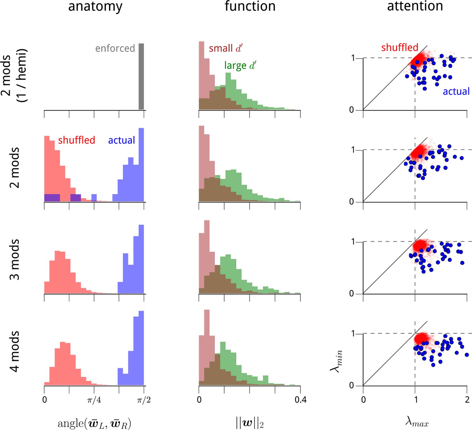
The structure of the modulators in higher-dimensional modulator models.
In the main text, we identify three striking properties of the two dominant shared modulators: (1) they each target one of the two V4 hemispheres; (2) they preferentially target the task-specific neurons within these hemispheres; and (3) their variance decreases under cued attention. Here we show that these features are present within higher-dimensional modulator models. In Figure 2—figure supplement 3, we show that these additional modulatory components do not convey any additional structure in these three domains. It is useful to first view the modulator model as a form of exponential-family Principal Component Analysis (PCA) (Collins et al., 2001; Solo and Pasha, 2013;Pfau et al., 2013). Standard PCA, like the shared modulator model, uncovers directions in signal space of maximal variation. However, PCA suffers from an identifiability problem: it can uniquely recover the subspace in which a small set of signals lie, but not the coordinate axes. PCA does select a particular orthogonal coordinate system to represent this subspace, but this solution is not unique, is sensitive to noise, and typically reveals little about the underlying generative process. This same identifiability problem is present with the shared modulator model. In the two-modulator case, we are able to resolve the ambiguity in the coordinate system by exploiting anatomical information (Figure 2b–c; see Materials and methods). However, the problem of identifiability becomes more acute in higher dimensions. Here, we show that the results presented in the main text for the 1-modulator/hemisphere model also hold for the unconstrained 2-modulator model. We also extend the 2-modulator results to the 3- and 4-modulator cases. This is necessary as, unlike standard PCA, the solutions to our equations in lower dimensions do not necessarily lie within subspaces of higher-dimensional solutions. This is because the regularization scheme and algorithm we use create biases that disrupt any strict nesting. We therefore need to explicitly test whether the structures we uncover in the 2-modulator model are also present in the 3- and 4-modulator models. And this needs to be done under the limitations of the identifiability problem, i.e. without choosing a particular coordinate system for the modulation subspace. First column: In Figure 2b–c, we showed that the vectors of modulator coupling weights for LHS units and RHS units in the 2D modulator model were typically orthogonal. Here we show that this holds in higher dimensions. For each recording day, we measured the angle between the average weight vector for LHS units (), and the average weight vector for RHS units (), i.e. the arc cosine of their inner product. The 2-modulator hemisphere-constrained model used in most of the main text has this orthogonality enforced by constraint (top row). For the unconstrained 2-, 3-, and 4-modulator models (remaining rows), the blue histograms show the distribution of these angles across recording days. For comparison, we shuffle the anatomical labels on each unit and repeat the analysis to obtain the red histograms. The clustering of the actual data around π/2 indicates near orthogonality of the hemispheric weights. Second column: In Figure 2d, we showed that neurons which were task-relevant (i.e. had larger d′ values) were more strongly coupled to the (1D) hemispheric shared modulators. Here, we show that this holds in higher dimensions. For each recording day, we measured the magnitudes of all units’ coupling weight vectors, . Green histograms show the distribution of magnitudes for the quartile of units with largest d′ values; brown histograms show the distribution of magnitudes for the quartile with the smallest d′ values. Third column: In Figure 3b, we showed that the variance of the (1D) hemispheric shared modulators changed according to the attentional cue: specifically, when the cue switched, one hemispheric modulator decreased in variance, while the other increased in variance. To show that this holds in higher dimensions, it is necessary to construct an appropriate metric for this change in second-order statistics that generalizes to higher dimensions, and that also does not depend on a choice of coordinate system. To accomplish this, we measure the effect of the attentional cue as a change in the covariance of the (multivariate) modulator. Considering the change from the cue-right to the cue-left condition, we can measure the effect on the modulator’s second-order statistics via the ratio of the two modulator covariances, . The eigenvalues of this matrix then provide a coordinate-system-free measure of how the modulator statistics change. If the largest eigenvalue, λmax, is significantly greater than 1, then there is a direction in modulation space that became more variable due to the switch in cue. If the smallest eigenvalue, λmin, is significantly less than 1, then there is a direction in modulation space that became less variable due to the switch in cue. Eigenvalues close to 1 indicate that the variance of modulation in that direction was unchanged by the cue. Thus these two values, λmax and λmin, play an analogous role to the ratios of modulator variance examined in Figure 3b. The scatter plots show the distribution of λmax and λmin for the higher-dimensional modulator models. Blue points show these eigenvalues from each recording day; red points show the distributions obtained if we shuffle the cue labels for each trial. Importantly, when λmax exceeds 1 and λmin is less than 1 (i.e. when the points lie in the lower right quadrant), then the change in attentional cue is causing an increase in modulator variance in one direction, and a decrease in modulator variance in an orthogonal direction. These effects are clear (and significant, compared with the null distribution in red) in all cases.
Figure 2—figure supplement 3
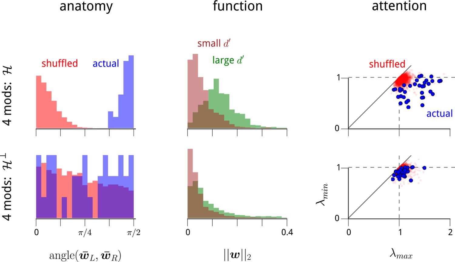
The modulators' anatomical, functional, and attentional structure manifests primarily within the dominant two dimensions of modulation.
In the main text, we recover a set of anatomical, functional, and attentional properties within a 2-dimensional modulator model. In Figure 2—figure supplement 2, we demonstrate that these properties also manifest within 3- and 4-modulator models. We wondered whether any additional structure can be seen in the extra two dimensions of modulation that we can include beyond the 2-modulator model. To answer this, we partitioned the 4-dimensional modulator space into two 2-dimensional halves. For each recording day, we define a particular 2D subspace of modulation along anatomical grounds. We measured the mean weight vectors for LHS and RHS units, and respectively. As shown in Figure 2—figure supplement 2, these two vectors were always near-orthogonal. We define their 2D span as the “hemispheric subspace of modulation”, . This is a 2D subspace of the 4D weight vectors, capturing the largest component of hemispheric-specificity in the modulator weights. What remains in the 4D modulation space is the hemispheric subspace’s orthogonal complement, . This divides the 4D space into two 2D subspaces, and thus amounts to a partial choice of a coordinate system. We can therefore study the anatomical and functional properties of the coupling weights in and , and also the attention-dependent statistics within the corresponding 2D spaces of time-varying modulator values. This panel shows that all three properties described in Figure 2—figure supplement 2 manifest predominantly in , but not in . In summary, each V4 hemisphere is being driven by a shared modulatory signal, that preferentially affects task-specific neurons, and has statistics that depend on the attentional cue provided to the animal. In addition, there is some evidence that other shared modulatory factors are affecting the population of V4 neurons. However, these latter signals do not share the same properties: their net effects are weaker, they do not appear to have the same anatomical or functional specificity, and they do not appear to be affected by the attentional cue.
Figure 2—figure supplement 4
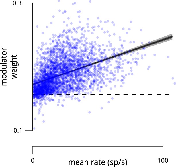
Units with higher mean firing rates typically had stronger coupling to their respective population modulator (r2 = 0.21).
This observation motivates the control analyses shown in Figure 2e, Figure 5—figure supplement 1 and Figure 8—figure supplement 1.
Figure 3
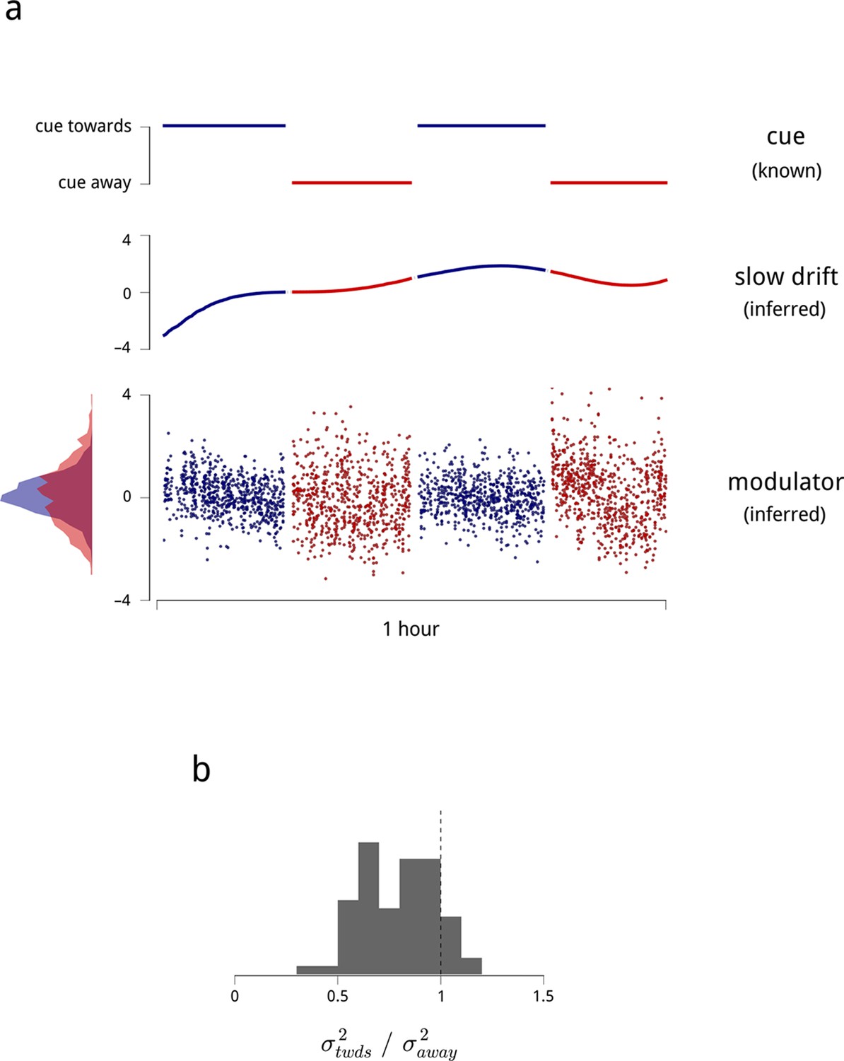
Time-varying model signals that determine the gain of units in one V4 hemisphere.
(a) Example values of the cue signal (imposed by experiment), the slow drift (inferred), and a single hemispheric modulator (inferred) across stimulus presentations for one day and hemisphere. In the model, the gain of each neuron is obtained by exponentiating a weighted sum of these three signals (see Equation (1)). Histogram in the bottom left shows the distribution of modulator values when the monkey was cued towards the contralateral side (blue), and away from it (red). (b) Modulator variance decreases under cued attention. Histogram shows the ratio of modulator variances estimated in the two cue conditions. Averaged across days and hemispheres, cued attention reduces modulator variance by 23%.
Figure 4

Changes in the statistics of the inferred modulator under cued attention explain the observed changes in spike count statistics.
(a) The classical model of attention. Simulation of two neurons with positive coupling weights, and , to the cue signal. When the cue is directed to the corresponding spatial location (top), both the mean and variance of the simulated neurons’ spike counts increase (bottom). Shaded areas demarcate analytic iso-density contours, i.e. the shape of the joint spike count distributions. (b) The effect of the shared modulator. Simulation of two simulated neurons with positive coupling weights, and , to a shared modulator. A decrease in modulator variance leads to a decrease in both the variance and correlation of spike counts (bottom). (c) Effects on an example pair of units within the same hemisphere, on one day of recording. The cue increases the gain of both cells (numbers indicate cue coupling weights), and the inferred modulator exhibits a decreased variance in cued trials (again numbers indicate coupling weights; top). The spiking responses of the cells exhibit a combination of the effects simulated in (a) in (b): increased mean, decreased Fano factor, and decreased correlation (bottom; means from 7.0 to 8.1 and 6.0 to 7.2 spikes/stim respectively; Fano factors from 1.9 to 1.6 and 1.7 to 1.6 respectively; correlation from 0.19 to 0.10). The shaded areas demarcate smoothed iso-density contours estimated from the data.
Figure 5 with 1 supplement
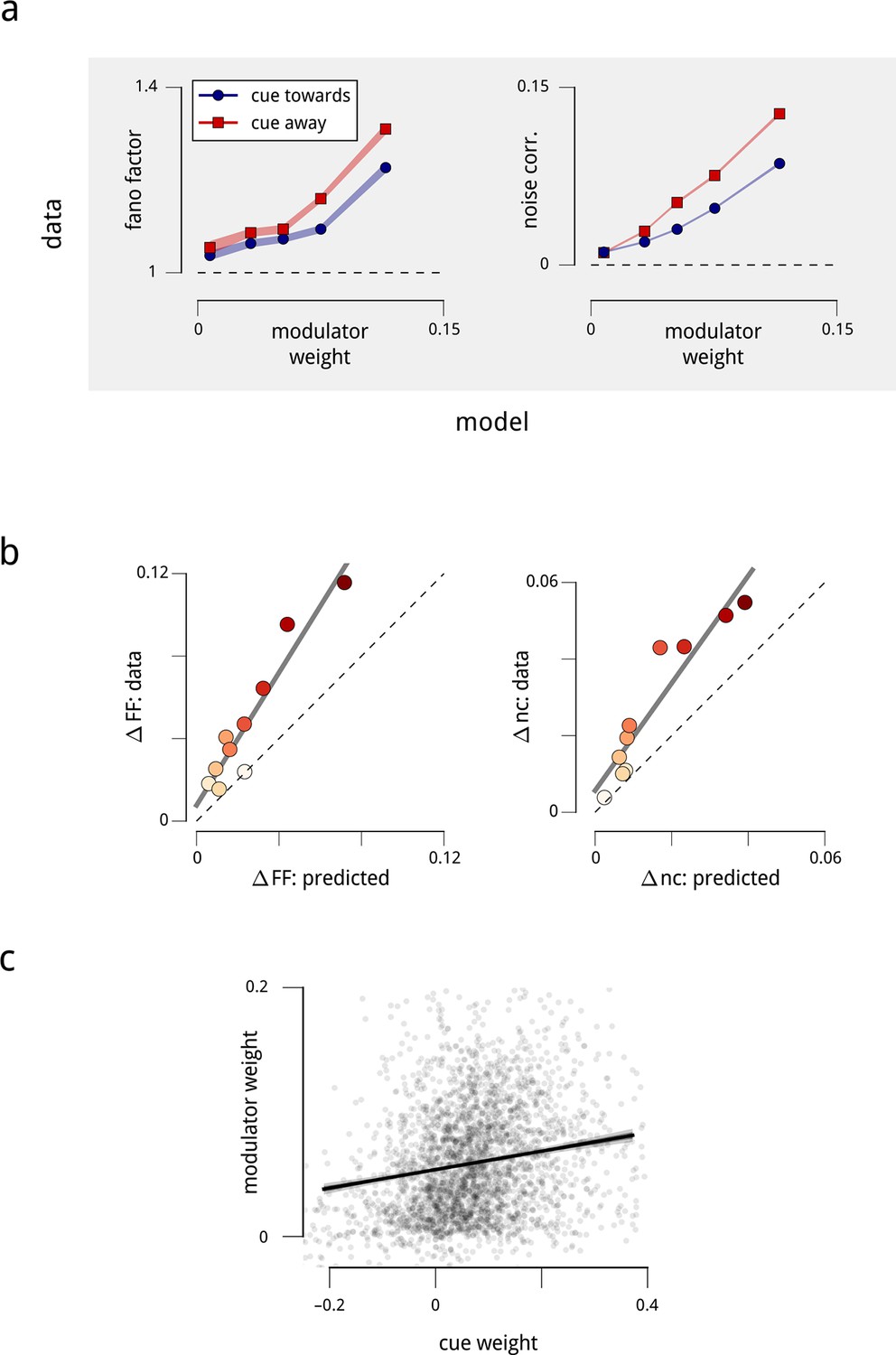
Attention-induced changes in neural response statistics are larger for neurons that are more strongly coupled to the shared modulator.
(a) Observed Fano factor and noise correlations, as a function of model coupling weight. Units from all days are divided into five groups, based on their fitted coupling weight to their respective population modulator (model-based quantities), as in Figure 2d. Points indicate the average Fano factors and noise correlations (model-free quantities) within each group, when attention was cued towards the associated visual hemifield (blue) and away from it (red). Shaded area denotes ± 1 standard error. Unitwise Spearman correlations: ρ = 0.31/0.44/0.40/0.51 (fano cue twds/fano cue away/ncorr cue twds/ncorr cue away). (b) Comparison of model-predicted vs. measured decrease in Fano factor and noise correlation. Units are divided into ten groups, based on coupling weights (darker points indicate larger weight). The model accounts for 62% of the cue-induced reduction in Fano factor, and 71% of the reduction in noise correlation. (c) Comparison of cue weights and modulator weights. Units that are strongly coupled to the cue signal are typically strongly coupled to the modulator signal, though the relationship is only partial (unitwise Spearman correlation: ρ = 0.26). These results are robust when controlled for firing rate (Figure 5—figure supplement 1).
Figure 5—figure supplement 1
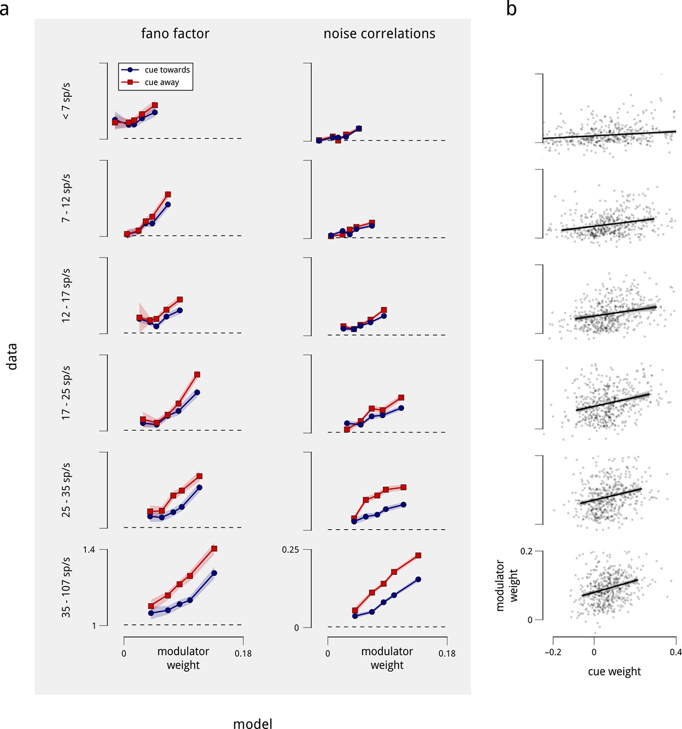
Differences in coupling weight explain the observed statistics of single and pairwise firing rates, even when controlled for mean firing rate.
The relationship shown in Figure 5 contains a potential confound in that units with higher mean firing rates are typically more strongly coupled to their corresponding shared modulators (Figure 2—figure supplement 4). Here, we perform the same analyses on subpopulations with similar mean firing rate. (a) We repeated the analysis of Figure 5a, but subdivided the total population of units in two ways: first, by mean firing rate into six groups (rows), and then by coupling weight into five subgroups (points on each plot). Each row thus replicates Figure 5a for a controlled subpopulation of approximately 500 units with similar firing rates. Within each group, the correlation between mean rate and modulator coupling weight was weak or negligible. Nevertheless, the relationships of Fano factor and noise correlation to modulator weight remain. (b) We also repeated the analysis of Figure 5b, subdividing the total population of units by mean firing rate into six groups, as in the rows of (a). Again, the relationship between cue and modulator weights remains.
Figure 6
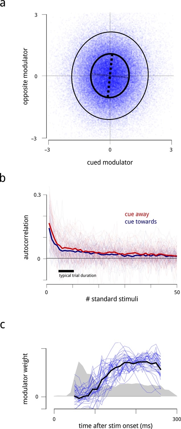
Statistical properties of the hemispheric modulators.
(a) Joint statistics of the two hemispheric modulators. Blue points: simultaneous values of the two modulators aggregated over all days. Thick black ellipse: iso-density contour at one standard deviation of the Gaussian density matching the empirical covariance. Thinner black ellipse: two standard deviations. Dashed lines: principal axes (eigenvectors) of this covariance, with the thicker dashed line indicating the axis with the larger eigenvalue. The vertical elongation of the ellipse shows that the variance of the modulator for the cued side is smaller than the variance of the modulator for the opposite side. The slight clockwise orientation shows that the two modulators have a very small positive correlation (, negligible). (b) Autocorrelation of modulators across successive stimulus conditions. Individual lines show the within-block autocorrelation of each estimated modulator; the thick lines shows the average across days and hemispheres. For simplicity of presentation, the targets and the gaps between trials have been ignored. The time constant of this process is on the order of several seconds. (c) Average time course of shared modulation within each stimulus presentation. We extended the population response model by allowing the value of the modulator to change over the course of each stimulus presentation. Given limitations of the data at fine temporal resolutions, we assumed that the temporal evolution of the modulator within each stimulus presentation followed some stereotyped pattern (up to a scale factor that could change from one stimulus presentation to the next; see Materials and methods). Fine blue lines: modulators’ (normalized) temporal structure extracted for each recording day. Heavy black line: average across days. Grey shaded area: normalized peri-stimulus time histogram (arbitrary units) of spiking responses during presentations of the standard stimuli, averaged across all units, days, and cue conditions, with zero denoting spontaneous rate. Shared modulation predominantly occurs during the sustained period and is nearly absent during the onset transient.
Figure 7 with 1 supplement
Inferred modulatory signals are predictive of behavioral performance, and are influenced by previous reward.
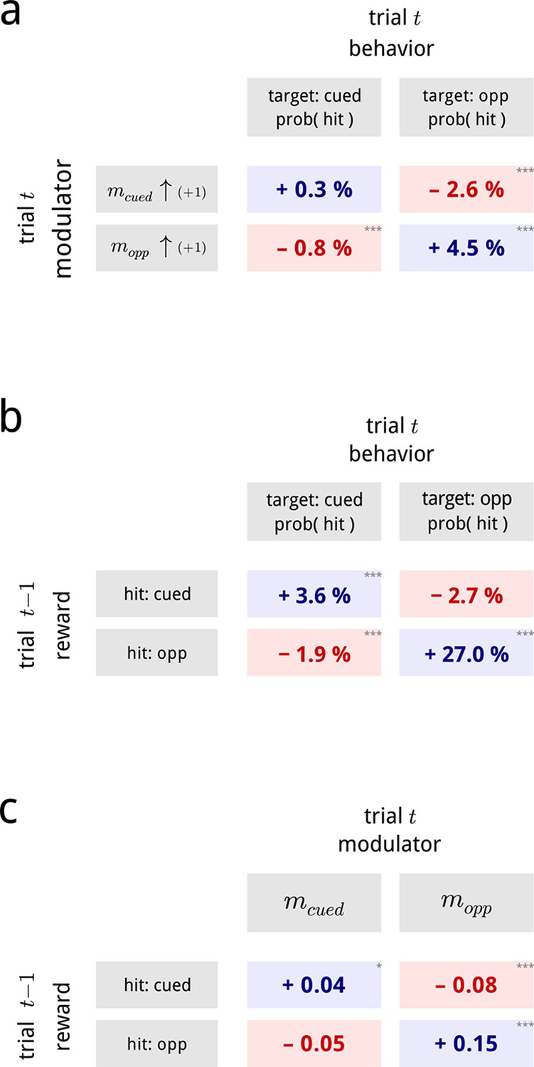
(a) Average effect of modulator values on subsequent behavioral performance, averaged across all days and difficulty levels. Values show the average change in hit probability for targets on the cued side (left column) and the opposite side (right column) following a unit increase in the cued (top row) and opposite (bottom row) modulators. *, **, ***. Full psychometric curves are shown in Figure 7—figure supplement 1a. (b) Average effects of previous trial reward on current trial performance. Note that this is a direct comparison of the behavioral data, and does not involve the modulator model. (c) Average effects of previous trial reward on the value of the two hemispheric shared modulators.
Figure 7—figure supplement 1
Relationship between modulators and behavior: additional details.
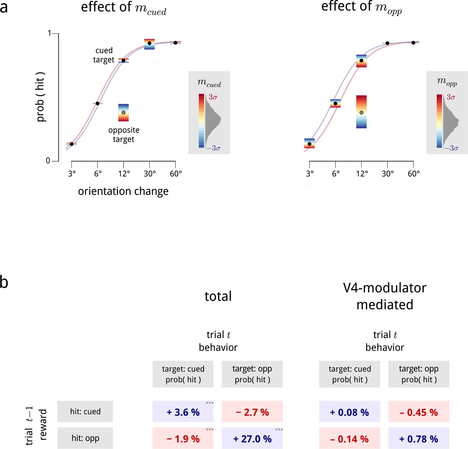
(a) Psychometric performance, averaged across all days. These plots expand the results of Figure 7 showing the interacting effects of trial difficulty and the two hemispheric modulators on task performance. The hit probability is shown as a function of the orientation change in degrees for trials where the target was on the cued side (black points) or the opposite side (single gray point; opposite side targets were only presented at 12 deg). For each condition, the color gradient shows the effects that values of the cued modulator (left panel) and opposite modulator (right panel) have on the hit probability. We fit a family of psychometric curves to the cued-target conditions, with the two modulator values as regressors; the colored lines in each panel show two of these curves, indicating the biasing effect of (left panel), and (right panel) on performance. (b) Left: average effects of previous trial reward on current trial performance, from Figure 7b. Note that this is a direct comparison of the behavioral data, and is not dependent on the modulator model. Right: effect of reward on performance predicted by chaining together the effects of reward on modulator (Figure 7a) and modulator on performance (Figure 7c). The biasing effect of reward on behavior, as mediated by the V4 modulators, is consistent with the observed data (left), but captures only a relatively small proportion of the total reward bias (∼5–10%). To estimate the total behavioral reward bias, we fitted Bernoulli-GLMs (i.e. GLMs with a Bernoulli observation process) which predict the response (hit/miss), given the previous trial’s reward (hit for target on cued side/hit for target on opposite side/other) as regressors. When the current trial’s target was cued, we treated the orientation change as an additional regressor, and we included a lapse parameter as behavioral performance typically saturated below 100% correct (Wichmann and Hill, 2001). The effect of previous reward in this model manifests as a bias term within the sigmoid (logistic) nonlinearity. To estimate the V4-mediated reward bias, we measured how large these total behavioral reward biases were if they had to pass through the “bottleneck” of the V4 modulators. We thus fitted three GLMs: a Gaussian-GLM which predicts the cued modulator on a trial, given the previous reward (and the previous modulator values); a second Gaussian-GLM which predicts the opposite modulator on a trial in the same way; and a Bernoulli-GLM which predicts the response (hit/miss), with the two modulators on that trial as a regressor. By multiplying these two effects together (the average change in modulators due to each previous reward state in the first and second GLMs, with the modulator coefficients in the third GLM), we obtained the desired quantities.
Figure 8 with 1 supplement
Interpreting the role of shared modulation.
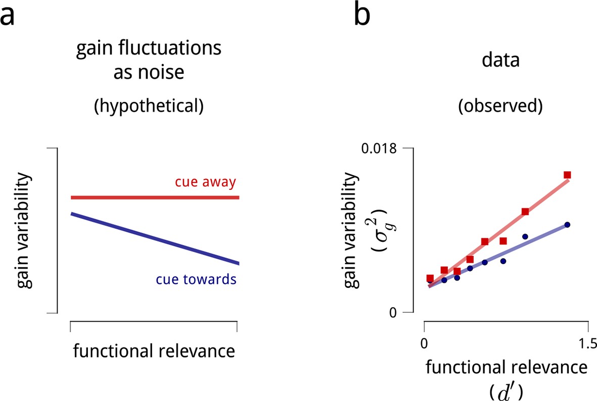
(a) Illustration of how shared gain fluctuations would behave if they were noise, i.e. undesirable random fluctuations. In baseline conditions (red), gain fluctuations would be expected to have similar variance for all neurons in the V4 population. The action of attention would be expected to reduce the variance of gain fluctuations in task-relevant neurons, so as to mitigate their adverse effect on coding precision (see Figure 4). (b) Contrary to this simple “noise” interpretation, the variance of shared gain fluctuations are markedly larger for task-relevant neurons than task-irrelevant neurons in baseline (cued away) conditions. Moreover, although this variance decreases under attentional cueing (cued toward), it remains larger for the task-relevant neurons. Functional relevance for each unit is measured as d′ (as in Figure 2d–e); shared gain variability, , is measured as the total variance of model-estimated gain fluctuations (from slow drift and modulators combined). These results are robust when controlled for firing rate (Figure 8—figure supplement 1).
Figure 8—figure supplement 1
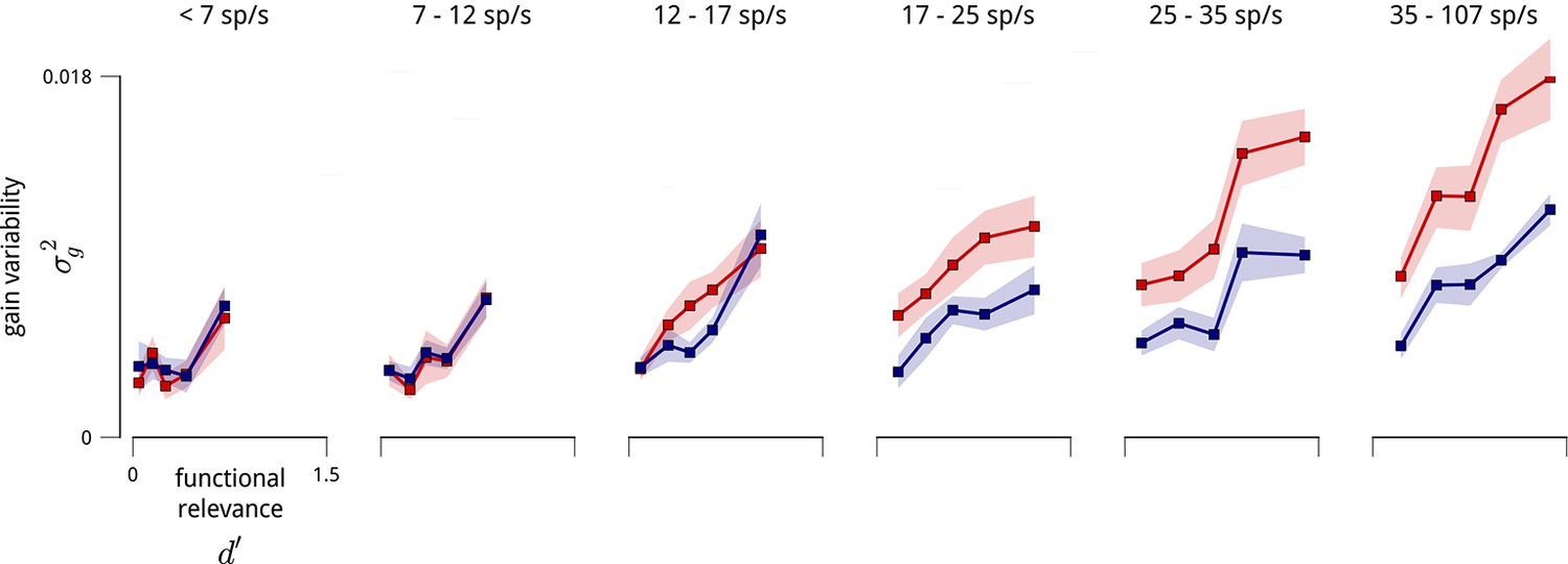
Variance of shared gain fluctuations is larger in task-relevant neurons, even when controlled for firing rate.
The relationship shown in Figure 8 contains a potential confound in that units with higher mean firing rates are typically more task-relevant, and also exhibit larger gain fluctuations. Here, we perform the same analyses on subpopulations with similar mean firing rate (subpopulations as in Figure 5—figure supplement 1).
Author response image 1
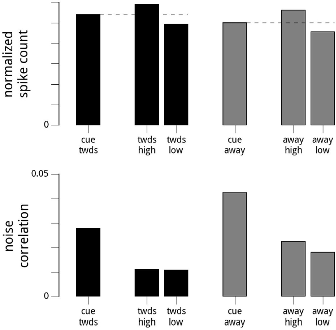
Suggested Analysis.
Here, we show the results of the reviewers’ suggested analysis. For each day and hemisphere, and within a given condition (cue towards, or cue away), we subdivide the data into two based on the values of the modulator (high modulator values, or low modulator values). We choose the threshold for the split so the variance of the modulator is the same for the two conditions. Top row: the mean firing rates are higher when conditioned on high modulator values. Bottom row: the noise correlations in the two subgroups are roughly equal (though still overall lower in the cue towards condition). Note that the subgroups’ noise correlations are lower than the full dataset for that cue condition, as we have reduced the (conditional) variance in the shared modulator. While this validates our statement that the noise correlations are the result of the variance of the shared modulator (since artificially reducing the variance of the shared modulator causes a dramatic reduction in the noise correlations), it does not resolve the status of whether the modulator is signal or noise.
Download links
A two-part list of links to download the article, or parts of the article, in various formats.
Downloads (link to download the article as PDF)
Open citations (links to open the citations from this article in various online reference manager services)
Cite this article (links to download the citations from this article in formats compatible with various reference manager tools)
Attention stabilizes the shared gain of V4 populations
eLife 4:e08998.
https://doi.org/10.7554/eLife.08998


