Figures and data in The evolution of distributed sensing and collective computation in animal populations | eLife

Figures
Videos

24 figures and 4 videos

Figures

Figure 1

Download asset Open asset

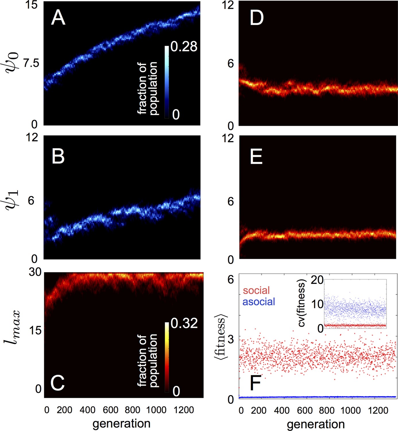
Evolution of behavioral rules.

(A, B) show evolutionary dynamics of populations of asocial individuals (i.e., maximum length scale of social interactions $l_{m a x}$ fixed; see text). (C-E) show evolutionary dynamics of individuals in which the maximum length scale of social interactions $l_{m a x}$ is allowed to evolve. Brightness of color indicates the frequency of a phenotype in the population. In asocial populations, baseline speed parameter $ψ_{0}$ (A) and environmental sensitivity $ψ_{1}$ (B) increase continually through evolutionary time. When $l_{m a x}$ is allowed to evolve (C), individuals quickly become social ( $l_{m a x}$ approaches maximum allowable value of 30), and baseline speed parameter $ψ_{0}$ (D) and environmental sensitivity $ψ_{1}$ (E) stabilize at intermediate values. Mean fitness of social populations (F, red points) is over five times higher than mean fitness of asocial populations (F, blue points), and the coefficient of variation in fitness is over four times lower in social populations (F inset). Unless otherwise noted, parameter values in all figures are as follows: $C = \frac{C_{r}}{C_{a}} = 1.1$ , $l = \frac{l_{r}}{l_{a}} = 0.13$ , $N = 500$ , $k = 25$ , $γ = 0.01$ , $τ = 1$ , $m = 1$ , $ν = 1$ , $ρ = 0.16$ , $M = 2$ , $λ_{0} = 10$ , $λ_{1} = \sqrt{20}$ , $α = (1,0)$ , $β = 0.1$ , and $τ_{p} = 1500$ .

https://doi.org/10.7554/eLife.10955.003

Figure 2

Download asset Open asset

Collective tracking of dynamic resource and length-scale matching.

(A) Sequence (left to right, top to bottom) of individuals interacting with moving resource peak (resource value in grayscale, darker = higher resource value). Peak is drifting to the right (grey arrow). Colors indicate the regime into which each agent falls (red: $Ψ > 2.95$ , blue: $0 < Ψ < 2.95$ , green: $Ψ < 0$ ). Length of tail is proportional to speed. Peak centroid moves according to 2D Brownian motion with drift (see Materials and methods). (B) When environments contain multiple resource peaks, evolved populations divide into groups that match peak sizes, e.g., in a two-peak environment, the size of group on each peak is proportional to peak size. Total size of two peaks is constant so that the larger the first peak (Peak 1, x-axis), the smaller the second peak. Peak size computed as the integral of the resource value over the entire peak (see Materials and methods). Group size is mean size of the group nearest each peak (mean taken over the last 2,500 time steps of each simulation). Points (and error bars) represent mean ( $\pm$ 2 standard errors) of 1,000 simulations for each combination of peak sizes. Parameters as in Figure 1 with $M = 2$ and values of $ψ_{0}$ , $ψ_{1}$ , and $l_{m a x}$ taken from a population in the ESSt.

https://doi.org/10.7554/eLife.10955.005

Figure 3

Download asset Open asset

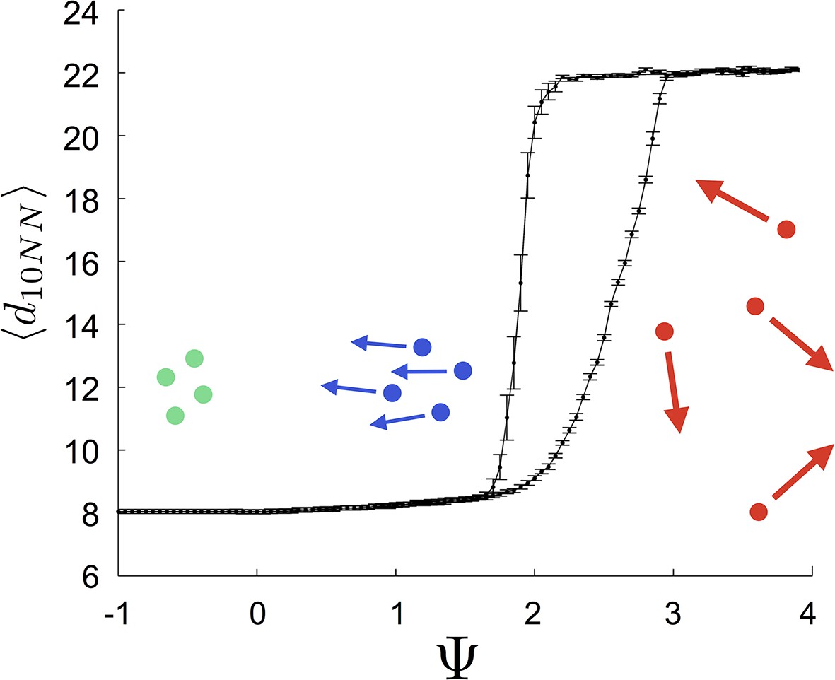
Hysteresis plot of the distance to 10 nearest neighbors, averaged over the entire population $⟨ d_{10 N N} ⟩$ (points and error bars) as a function of preferred speed parameter $Ψ$ in a uniform environment.

Figure produced by starting with a population with $Ψ = 4$ in a uniform environment. Population is allowed to equilibrate for 5000 time steps and $⟨ d_{10 N N} ⟩$ is then computed. $Ψ$ is then lowered. This process is repeated until $Ψ = - 1$ , at which point the same procedure is used to increase $Ψ$ . Upper curve corresponds to decreasing $Ψ$ . Lower curve corresponds to increasing $Ψ$ . Regimes where $Ψ ~ 0$ and $Ψ \in (1.6,2.95)$ correspond to transitions between collective states. Points and (error bars) correspond to mean ( $\pm$ 2 standard errors) of 50 replicate simulations. Parameters as in Figure 1 with $l_{max} = 30$ .

https://doi.org/10.7554/eLife.10955.007

Figure 4

Download asset Open asset

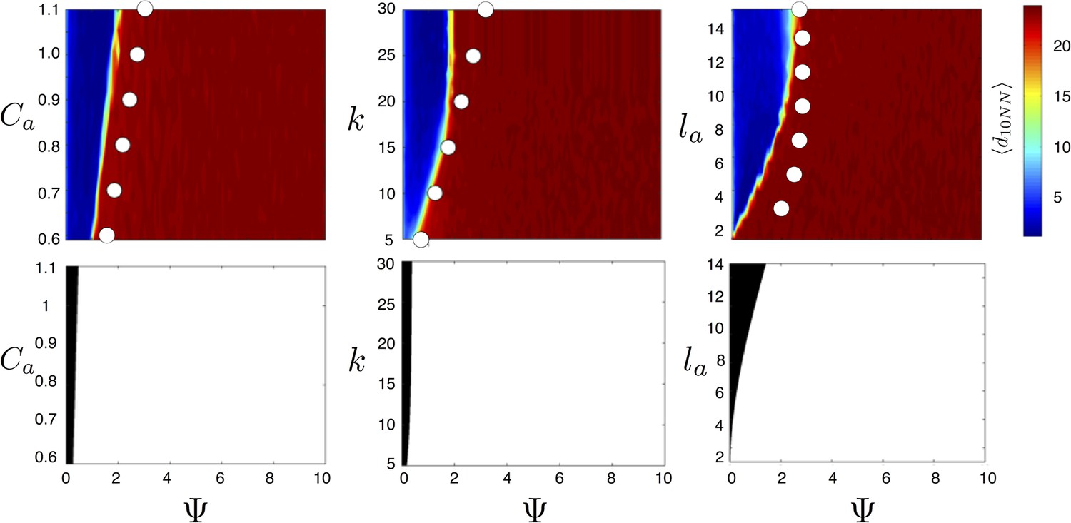
Evolved populations are positioned near transitions in collective state.

Upper panels show mean distance to 10 nearest neighbors ( $⟨ d_{10 N N} ⟩$ , color scale) from simulated populations. A separate populations is simulated in a uniform environment for each value of the social attraction strength ( $C_{a}$ ), number of neighbors an individual reacts to ( $k$ ), and the decay length of social attraction ( $l_{a}$ ) parameters. Red is low density corresponding to dispersed state, and blue is high density corresponding to cohesive state. Points show the mean value of $ψ_{0}$ of populations in the EESt (populations evolved for 1,000 generations in an environment with dynamic resource peaks). Evolved populations are positioned near transition between cohesive and dispersed states. Lower panels are based on analytical calculations and show the predicted regions in which the dispersed state is stable (white) and unstable (black, Appendix section 5). Parameters as in Figure 1 with $M = 15$ , $λ_{0} = 10$ , $λ_{1} = 1.6$ , $α = (1,0)$ , $β = 0.1$ , and $τ_{p} = 1500$ .

https://doi.org/10.7554/eLife.10955.008

Figure 5

Download asset Open asset

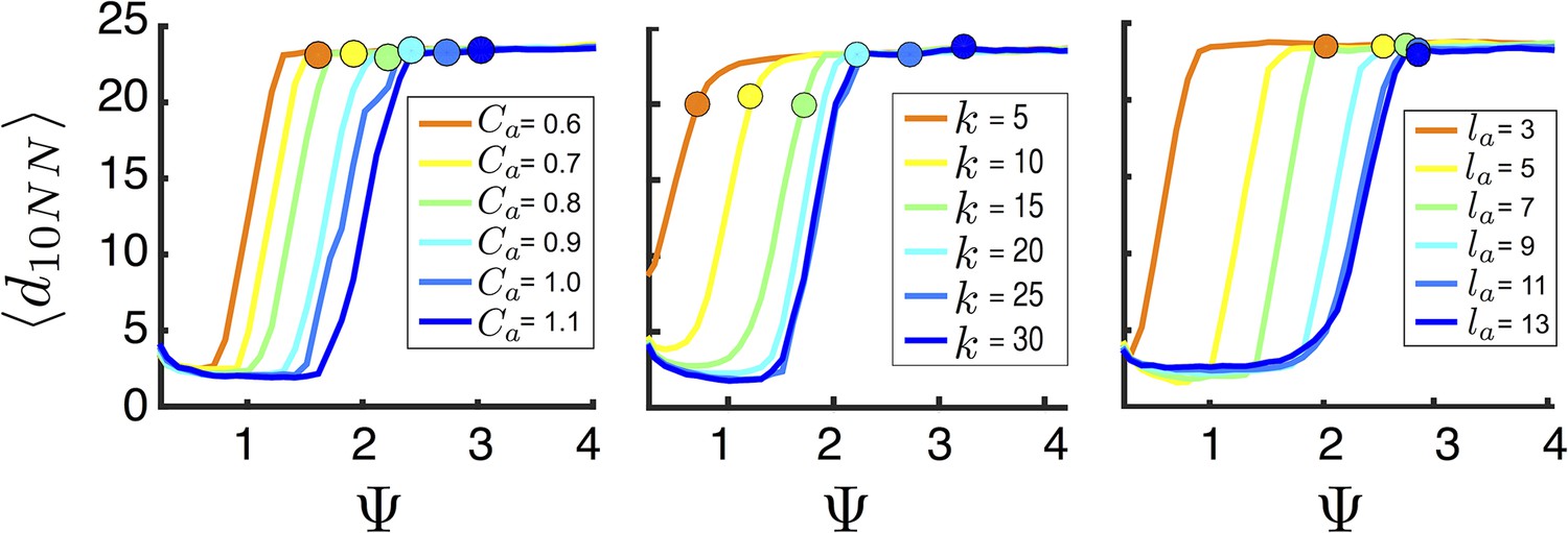
Mean distance to nearest neighbors $⟨ d_{10 N N} ⟩$ (curves) and ESSt value of $ψ_{0}$ (points) as a function of social parameters.

Points denote mean ESSt value of $ψ_{0}$ . Note abrupt transitions in density as function of $Ψ$ , as shown in Figure 3. In all cases, ESSt value of $ψ_{1}$ causes populations to cross transition when resource value is high (i.e., $ψ_{0} - ψ_{1} λ_{0} < 0$ , where $λ_{0}$ is maximum resource value of each peak). Densities and ESSt values generated as described in Figure 4.

https://doi.org/10.7554/eLife.10955.009

Figure 6

Download asset Open asset

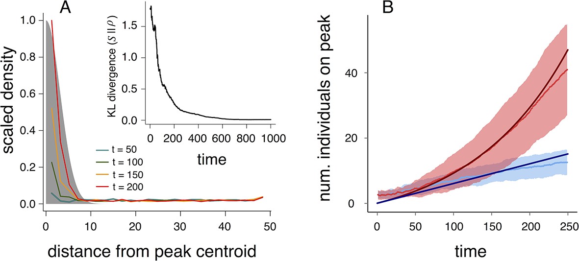
Collective computation and social gradient climbing.

(A) Collective computation of the resource distribution (grayscale represents resource value, normalized to maximum of 1). Curves show local density of individuals at different distances from the resource peak center (maximum value also normalized to 1). Note the rapid accumulation of individuals near the peak center. The distribution of individuals becomes increasingly concentrated in the region where the resource level is highest; inset shows that the Kullback-Leibler divergence between the resource distribution and the local density of individuals decreases through time as the two distributions become more similar. (B) Number of individuals near peak center (within one decay length, $λ_{1}$ , of peak center) as a function of time. Red and blue points and confidence bands represent means $\pm 1$ sd. for 100 replicate simulations. Red points and band is ESSt population and blue points and band is an asocial population with the same parameter values. Curves are analytical predictions based on Equations 3 and 4 (Appendix section 6).

https://doi.org/10.7554/eLife.10955.010

Appendix Figure 1

Download asset Open asset

Speeding force as a function of the location of a single neighbor.

On the left of the origin, the neighbor is behind the focal individual. For very short distances, the neighbor exerts a positive speeding force on the focal individual, causing it to accelerate. For longer negative distances, the speeding force on the focal individual is negative; the focal individual decelerates to come closer to its neighbor. To the right of the origin the neighbor is in front of the focal individual. For short distances, the speeding force on the focal individual is negative, causing it to slow down. For longer positive distances the speeding force exerted on the focal individual is positive; the focal individual speeds up, closing the distance between it and its neighbor. The distance corresponding to repulsion only is shown with the blue line. Parameters as follows: C_a = 1, C_r= 1.1, l_a= 3, l_r= 1.

https://doi.org/10.7554/eLife.10955.013

Appendix Figure 2

Download asset Open asset

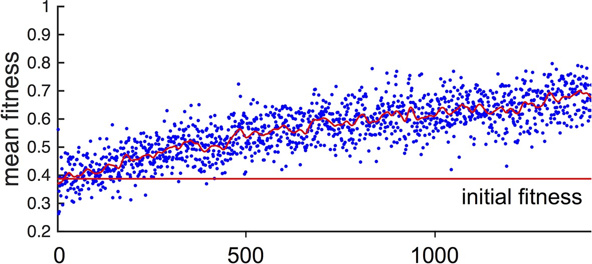
Fitness of asocial population through evolutionary time.

Blue points indicate mean fitness of population in each generation. Horizontal red line indicates mean fitness of population over first ten generations. Corresponding $ψ_{0}$ and $ψ_{1}$ values for each generation are shown in Figure 1A,B of the Main Text.

https://doi.org/10.7554/eLife.10955.014

Appendix Figure 3

Download asset Open asset

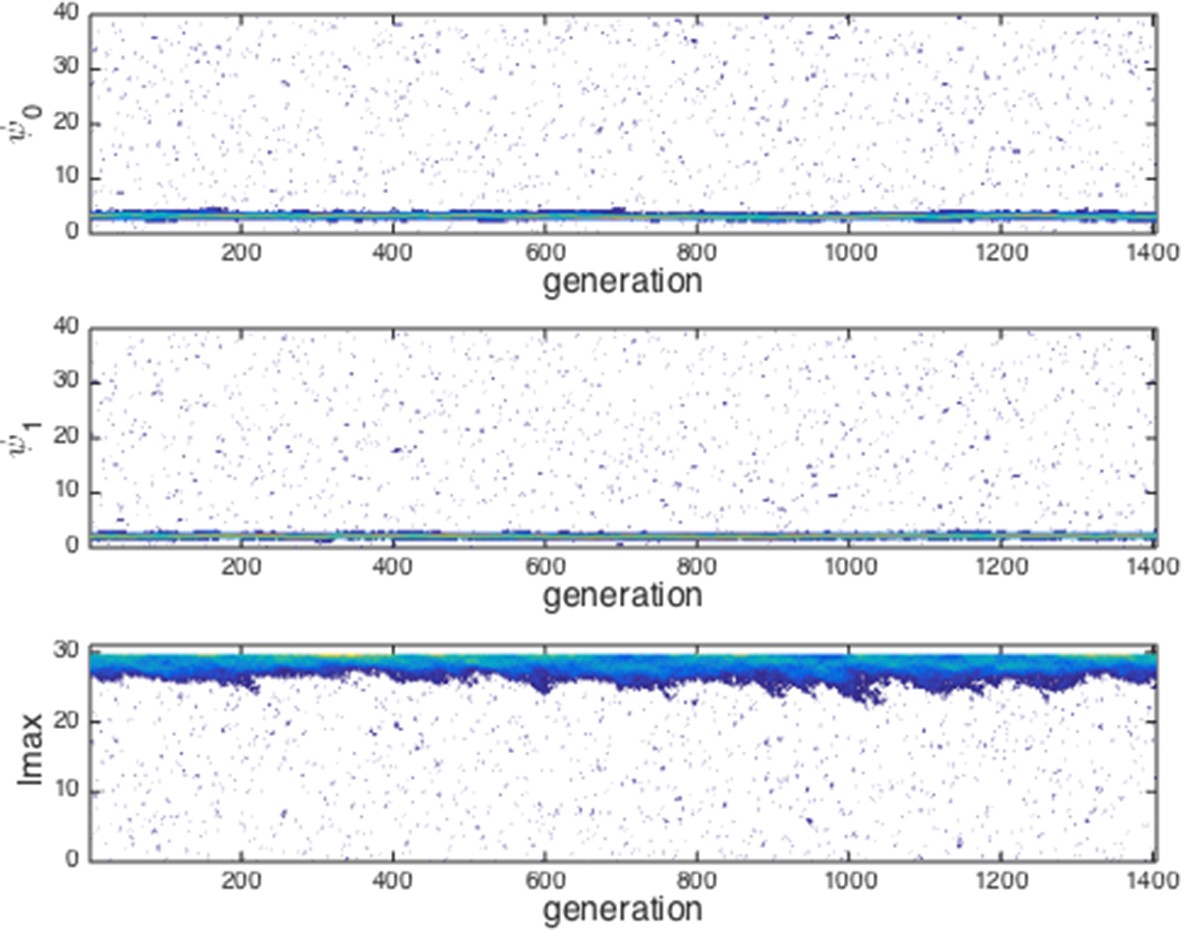
Evolution of traits under invasion by mutants far from the ESSt.

Example evolutionary progression for $ψ_{0}$ , $ψ_{1}$ and $l_{m a x}$ . Note that invaders (blue points introduced across phenotype space) do not establish and the dominant trait values in the population do not change over evolutionary time. Color indicates frequency of phenotype in population (white = 0, blue = low frequency, orange = high frequency).

https://doi.org/10.7554/eLife.10955.015

Appendix Figure 4

Download asset Open asset

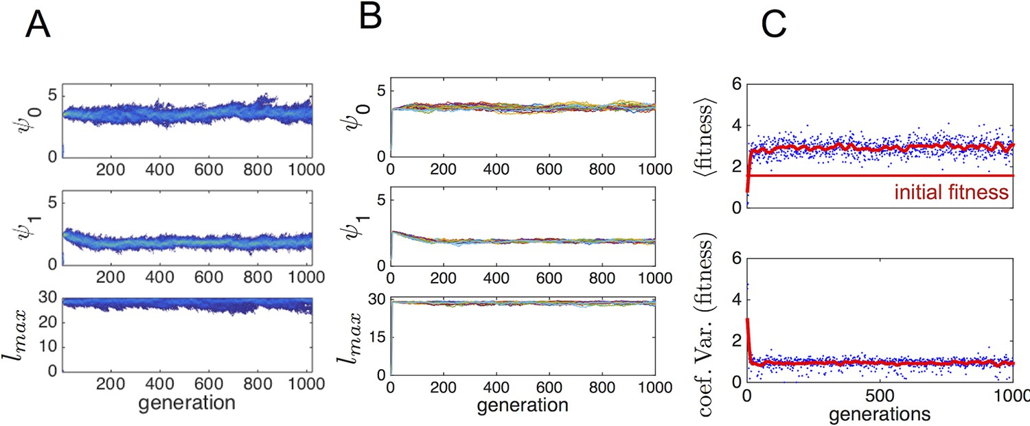
Typical progression of evolution from initial state with N − 1 asocial individuals and individual selected from the ESSt population.

(A) Invader from ESSt increases in abundance and sweeps population. (B) Mean trait values in 50 replicate invasions (each line is a separate invasion from the same initial state with N − 1 asocial individuals). ESSt phenotype quickly invades and sweeps the population in all cases. (C) Mean and coeffient of variation in fitness corresponding to the invasion shown in A.

https://doi.org/10.7554/eLife.10955.016

Appendix Figure 5

Download asset Open asset

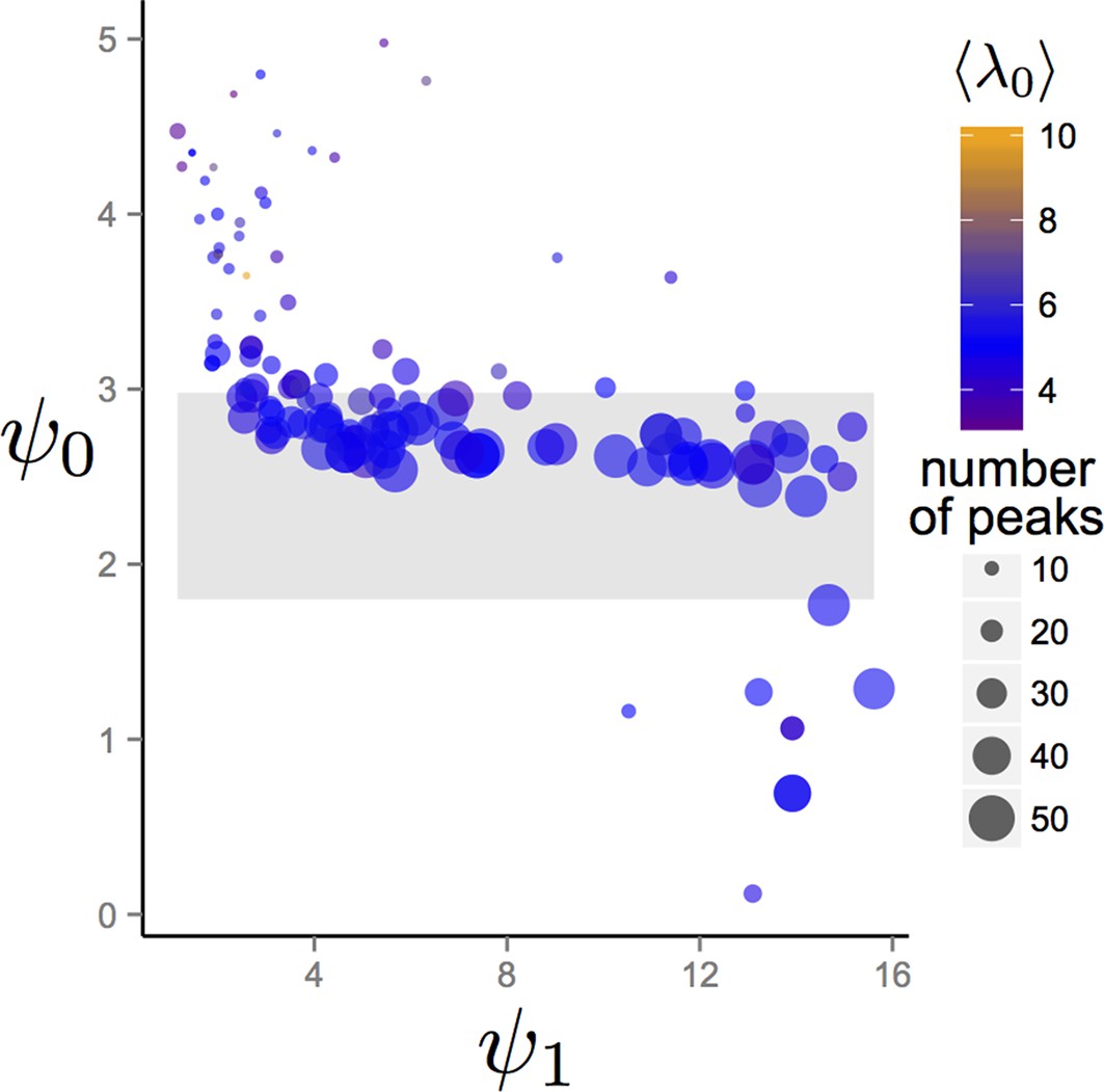
Trait values after 1500 generations of evolution in randomly generated environments.

Each point represents the mean trait values of a single population that has been allowed to evolve for 1500 generations. Point sizes denote the number of peaks that were present in the environment. Point colors represent the maximum resource value λ₀ averaged over all peaks present in the environment. Gray region corresponds to the region of hysteresis shown in Figure 3 of the Main Text. Number of peaks and peak parameters were chosen at random. All other parameters as in Figure 1 of Main Text.

https://doi.org/10.7554/eLife.10955.017

Appendix Figure 6

Download asset Open asset

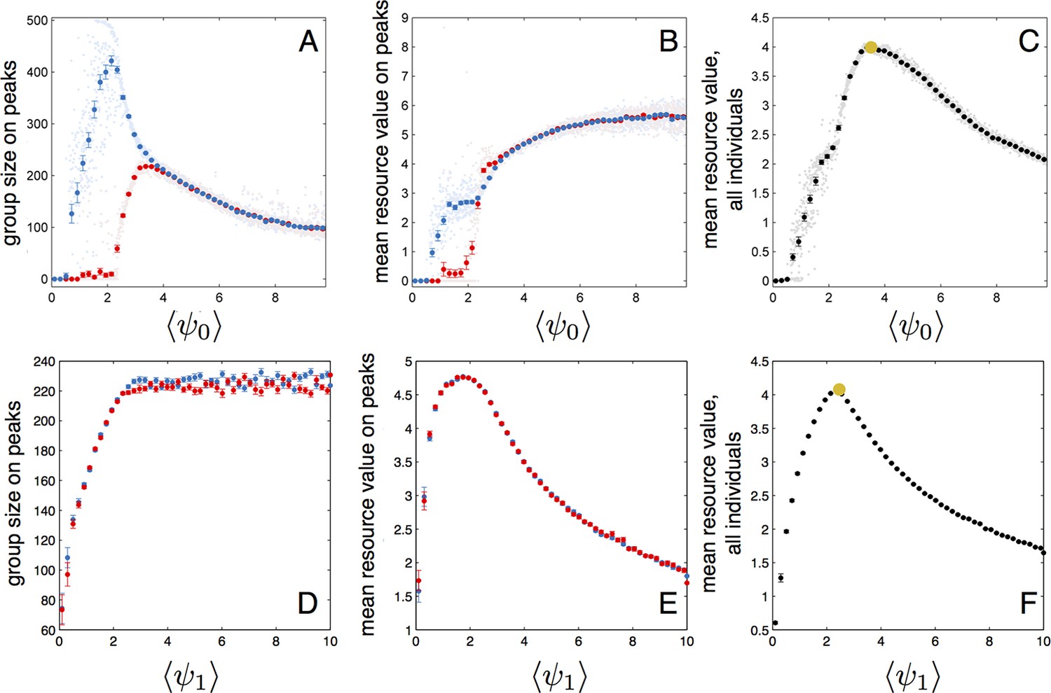
Performance of populations near the evolutionarily stable state.

(A) The number of individuals on each peak (the starting peak, blue; the second peak, red) as a function of the mean baseline speed parameter, $ψ_{0}$ of a population perturbed from the ESSt. Below a $ψ_{0}$ of roughly 2.2, individuals do not form a large group on the second peak. (B) Mean resource value of individuals on the starting peak (blue) and second peak (red). (C) Resource value averaged over all individuals in the population (individuals in groups nearest each peak and all other individuals in the environment). Note maximum value occurs in the regime where individuals aggregate on both the starting and second peaks ( $ψ_{0} ~$ 3.6). Orange point indicates values corresponding to ESSt. (D-F) Group size (D), mean resource value of individuals on peaks (E), and mean resource value of all individuals (F) as a function of the mean environmental sensitivity parameter $ψ_{1}$ of a population perturbed from ESSt. Orange point in (F) indicates values corresponding to ESSt. Note rapid decrease in mean fitness for perturbations in both directions. Semitransparent points are results of 2000 individual simulation runs. To compute means and standard errors, simulation runs were divided into 50 evenly spaced bins. Bolded points and error bars show mean of each bin $\pm$ 2 standard errors.

https://doi.org/10.7554/eLife.10955.018

Appendix Figure 7

Download asset Open asset

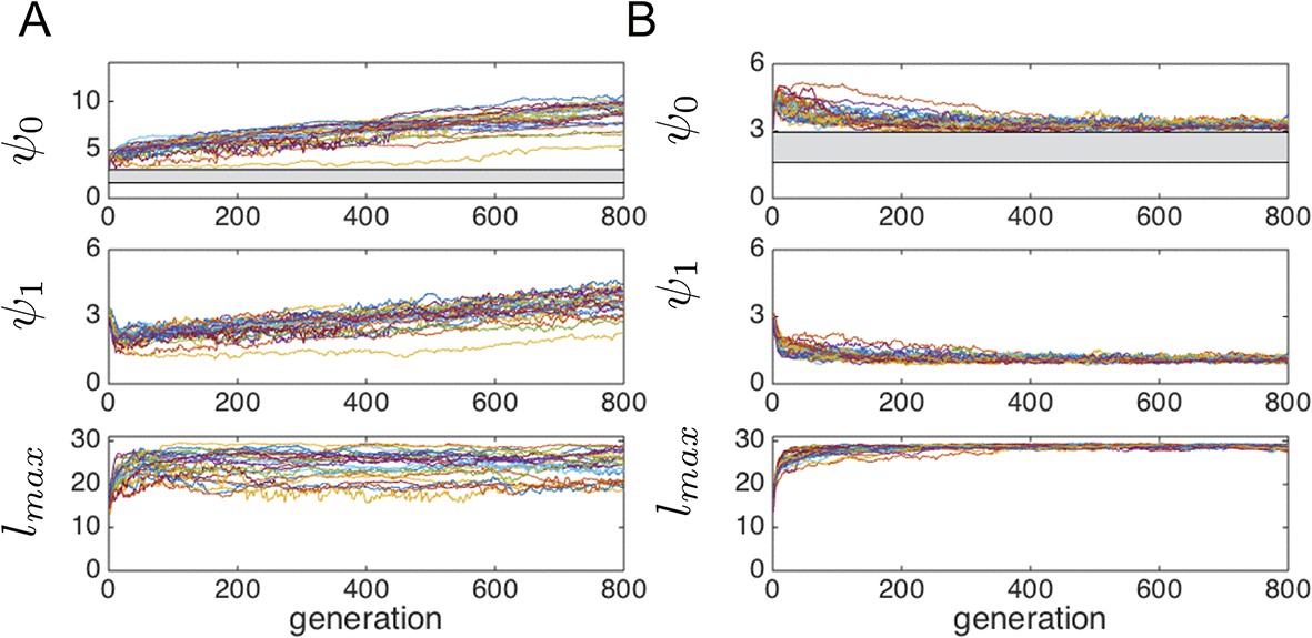
Evolution of behavioral traits when individuals consume resource.

Lines show means of independent evolutionary simulations. (A) High consumption rate corresponding to fast depletion of resource peaks. (B) Intermediate consumption rate corresponding to slower depletion of the peaks. Note different axis limits in the top panels of A and B. Grey region corresponds to hysteresis region between collective states shown in Main Text Figure 3. Parameters are as follows: s*=2, high consumption rate = 3.2*10^–3 (time step⁻¹), low consumption rate = 8.0*10^–5 (time step⁻¹), N = 300. All other parameters as in Figure 1 of the Main Text. These consumption rates correspond to the case where 100 individuals near the peak center can deplete a peak in roughly five time steps (fast depletion, A), and the case where the same task takes 200 time steps (slower depletion, B).

https://doi.org/10.7554/eLife.10955.019

Appendix Figure 8

Download asset Open asset

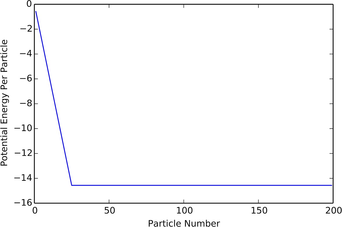
Plot of potential energy per agent as a function of group size.

Cutoff at N = K indicates constant density.

https://doi.org/10.7554/eLife.10955.020

Appendix Figure 9

Download asset Open asset

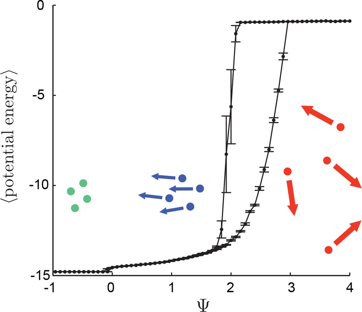
Hysteresis plot of potential energy averaged over the entire population (compare with Figure 3 in Main Text).

Figure produced by starting with a population with Ψ = 4 in a uniform environment. Population is allowed to equilibrate for 5,000 time steps and then average potential energy is calculated using Equation 4 in the Main Text. Ψ is then lowered. This process is repeated until Ψ = −1, at which point the same procedure is used to increase Ψ. Upper curve corresponds to decreasing Ψ. Lower curve corresponds to increasing Ψ. Note drop in mean potential energy at Ψ = 0. We refer to the states on either side of this transition as station-keeping (Ψ < 0) and cohesive Ψ > 0 and below upper transitional regime at Ψ ∼ 1.7. Points and (error bars) correspond to mean (and 2 standard errors) of 50 replicate simulations. Parameters as in Figure 1 of the Main Text with l_max = 30.

https://doi.org/10.7554/eLife.10955.021

Appendix figure 10

Download asset Open asset

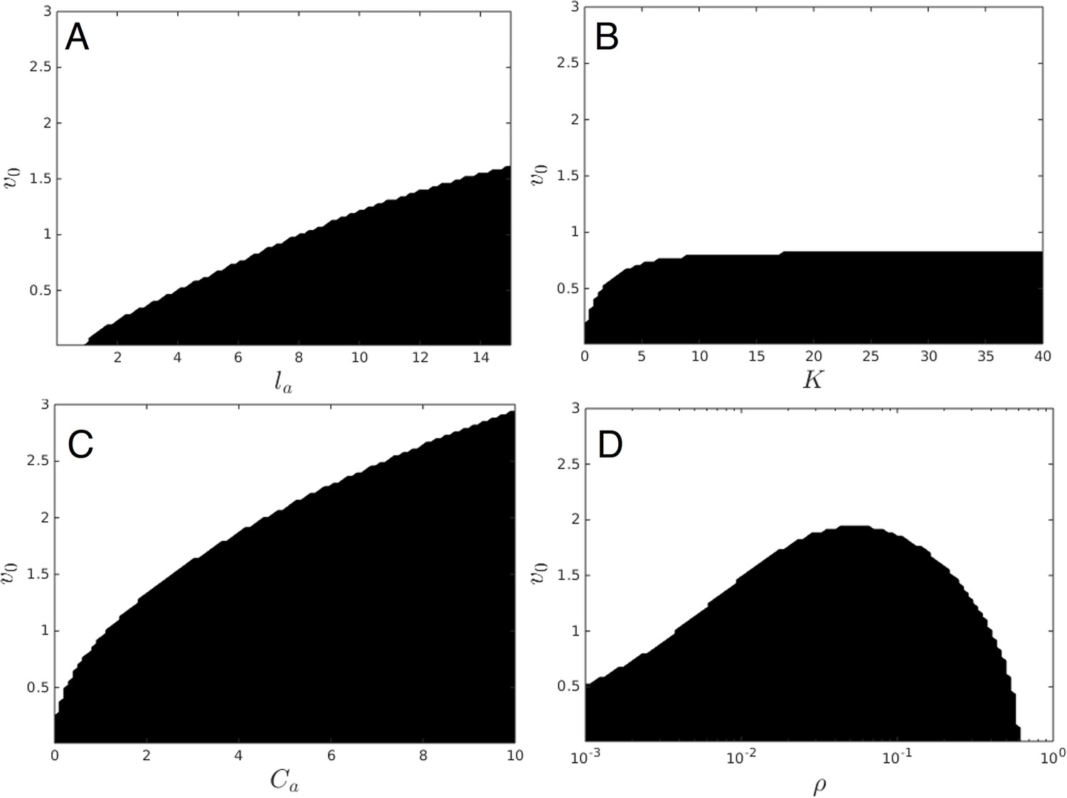
Regions of parameter space where dispersed state is stable (white) and unstable (black).

Instability of dispersed state causes transition to cohesive state. (A) Sensitivity to l_a, for ρ = .0025, K = 25, l_r = 1.0, C_a= 1.0, C_r= 1.1. Increasing l_a promotes instability and formation of the cohesive state, as does decreased v₀. (B) Sensitivity to K, for ρ = .0025, l_a = 7.5, l_r = 1.0, C_a= 1.0, C_r= 1.1. Increasing K promotes instability and formation of the cohesive state, as does decreased v₀. Large values of K lead to roughly the same stability properties, due to the exponential decay of the interaction with length. (C) Sensitivity to C_a, for ρ = .0025, l_a = 7.5, l_r = 1.0, K = 25, C_r= 1.1. Increasing C_a promotes instability and formation of the cohesive state, as does decreased v₀. (D) Sensitivity to ρ. Smaller v₀ promotes instability. When ρ is very small, increasing ρ makes instability more likely.

https://doi.org/10.7554/eLife.10955.022

Appendix Figure 11

Download asset Open asset

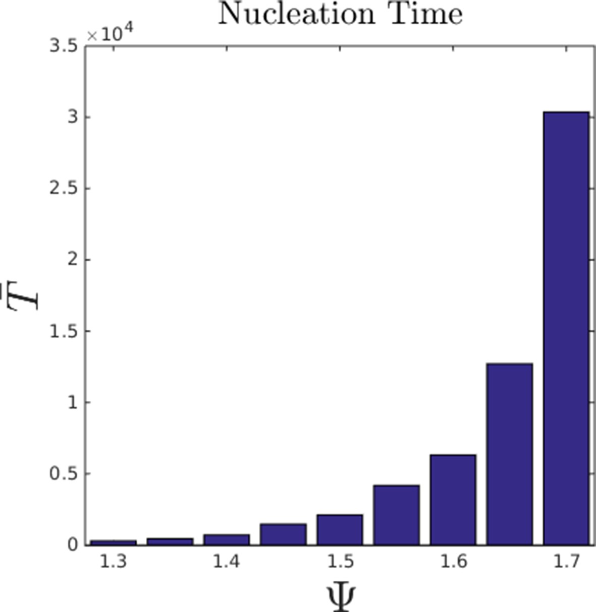
Mean nucleation time as a function of Ψ in the hysteresis region.

Bars show mean nucleation time calculated from replicate simulations in which individuals begin the simulation with random starting positions. Simulation was ended when an agent reached a social potential value < −14, which is only possible if a dense group has formed. For each simulation, we denoted the time taken to satisfy this condition as the nucleation time. Parameter values taken from population at ESSt described above.

https://doi.org/10.7554/eLife.10955.023

Appendix Figure 12

Download asset Open asset

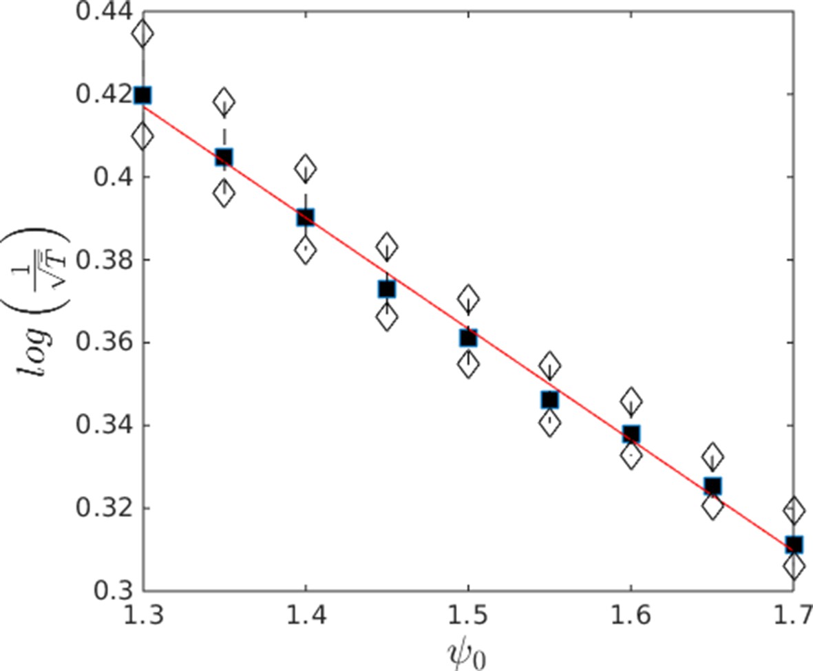
Approximate scaling of mean nucleation time with Ψ in the hysteresis region.

Data from Appendix Figure 11. Black points show means. White points are ± 1 standard deviation. Note that the nucleation time is super-exponential in Ψ indicating that the probability of nucleation becomes extremely small as Ψ approaches the upper boundary of the hysteresis region.

https://doi.org/10.7554/eLife.10955.024

Appendix Figure 13

Download asset Open asset

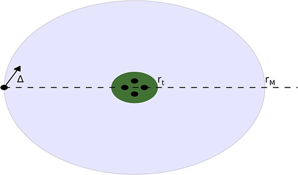
There is a group agents on the resource peak at the origin.

These agents are contained within the a circle of radius r_t, corresponding to the zero velocity region. An agent enters the region of radius r_M and begins to feel the force from the agents on the peak. The angle of the velocity of the agent relative to the peak is ∆.

https://doi.org/10.7554/eLife.10955.025

Appendix Figure 14

Download asset Open asset

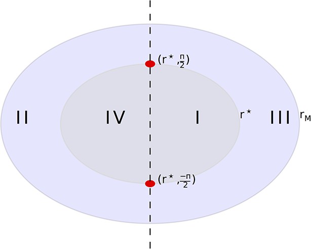
Division of the (r, ∆) plane into trapping and escaping regions.

Any particle that enters region I will eventually reach the zero velocity radius. Any particle that enters region II will escape capture by the peak. Our initial condition will be in the right half plane, on the circle of width r_M. The two red circles are unstable equilibria, each corresponding to a circular orbit of the peak.

https://doi.org/10.7554/eLife.10955.026

Appendix Figure 15

Download asset Open asset

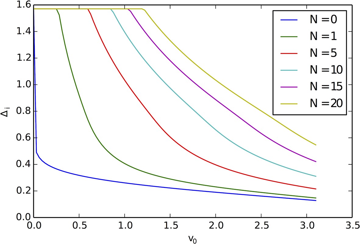
Critical angle $∆_{i}$ for capture of agents by the resource peak, for different peak occupancy levels N and different values of the background velocity $v_{0} = \sqrt{ψ_{0}}$ .

Small v₀and large N lead to increased $∆_{i}$ and a greater cross-section for capture of agents by the resource peak.

https://doi.org/10.7554/eLife.10955.027

Appendix Figure 16

Download asset Open asset

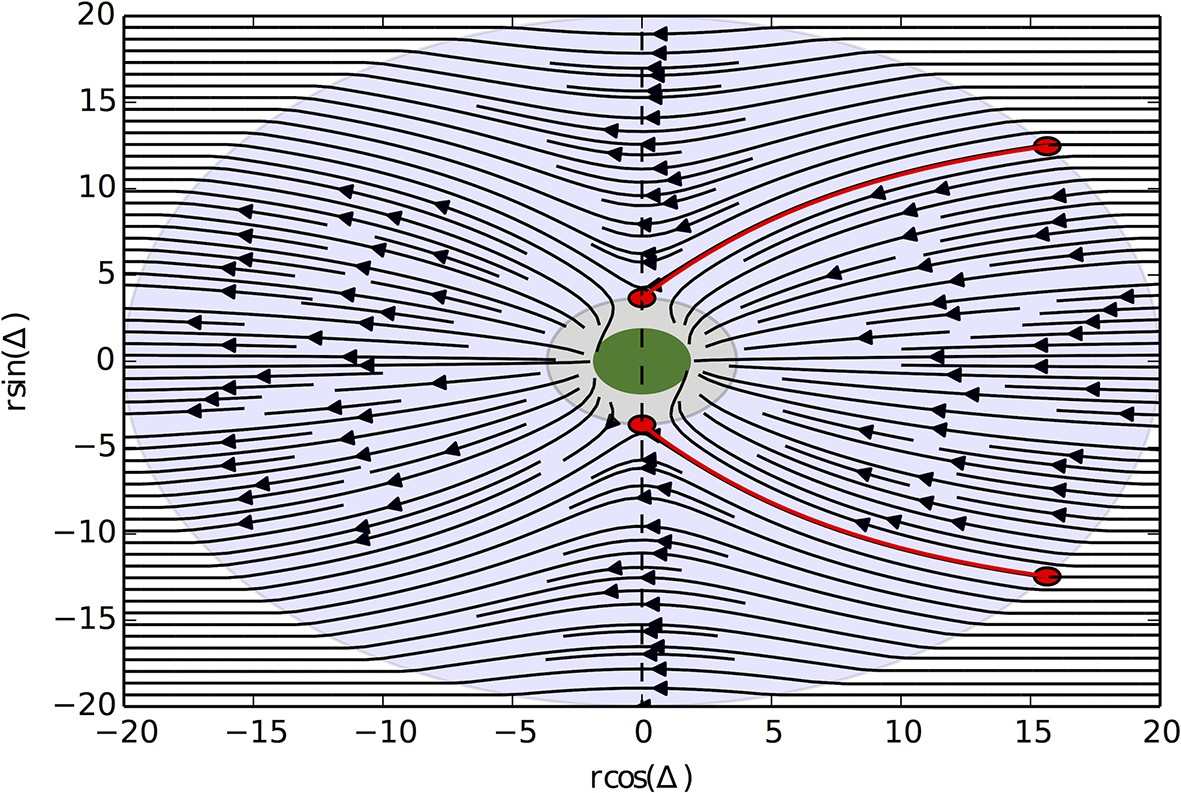
Solutions of the differential equation for $v_{0} = 2.0$ and N = 8.

The green region corresponds to 0 velocity. In the grey region surrounding the green region, the potential is stronger than centrifugal forces, which for $- \frac{π}{2} < ∆ < \frac{π}{2}$ represents the trapping region. The two red circles correspond to the unstable equilibrium points, and the red trajectories are the trajectories that begin at $(\pm ∆_{i}, r_{M})$ , which reach the equilibrium points and thus represent the boundaries of the set of initial conditions that are captured.

https://doi.org/10.7554/eLife.10955.028

Appendix Figure 17

Download asset Open asset

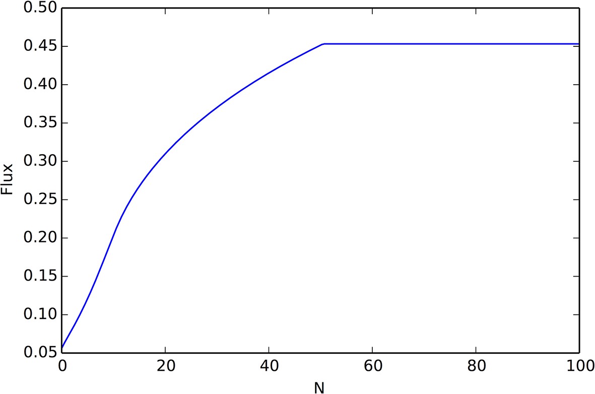
Rate of arrival of social agents onto a resource peak as a function of the number of agents already on the peak.

There are two behavior regimes, the initial regime in which flux grows linearly with N (giving rise to exponential growth of the number of individuals on the peak), and a regime where the flux reaches it’s maximum value (after which point peak occupancy grows linearly). This figure was calculated using Equation A67, with velocity v₀= 1.0, density ρ = .01, K = 25 interaction neighbors, social potential min(N, K)e^−|r|/7.5, and resource peak shape $10 e^{- | r^{2} | / 25.0}$ .

https://doi.org/10.7554/eLife.10955.029

Appendix Figure 18

Download asset Open asset

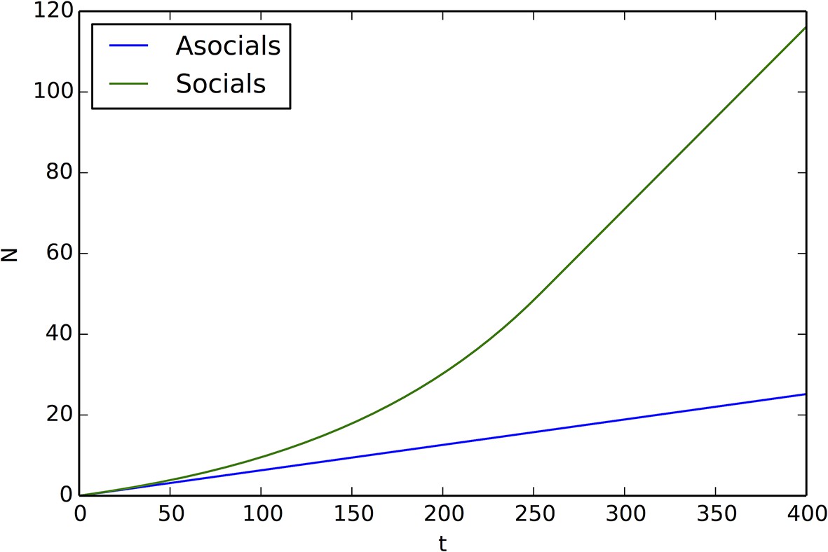
Comparison of peak occupancy as a function of time between social and asocial agents, using the parameters that generated Appendix Figure 17 and Equation A66, A69, A71.

Social agents occupy the peak much more quickly than asocial agents.

https://doi.org/10.7554/eLife.10955.030

Videos

Video 1

Download asset

posterframe for video — Asocial population.

Responses of population of asocial individuals (points) and dynamic resource peak (resource value shown in grayscale; dark regions have high resource value, light regions have low resource value). Length of tail proportional to speed. Peak centroid moves according to 2D Brownian motion with drift vector $α$ and standard deviation $β$ (see Materials and methods). In Videos 1–4, view is zoomed in to area surrounding moving resource peak (field of view is $50 l_{r} \times 50 l_{r}$ , where $l_{r}$ is the length scale of repulsion; full environment is projected onto a torus with edge length $346 l_{r}$ ). Behavioral parameters as follows: $C_{r} = 1.1$ , $C_{a} = 1$ , $l_{r} = 1$ , $l_{a} = 7.5$ , $γ = 0.01$ , $τ = 1$ , $m = 1$ , $η = 1$ , $ψ_{0} = 3$ , $ψ_{1} = 2.54$ . Environmental parameters in Videos 1–4 are: $ρ = 0.16$ , $N = 300$ , $M = 2$ , $λ_{0} = 10$ , $λ_{1} = \sqrt{20}$ , $α = [0.06 0]$ , $β = 0.5$ .

https://doi.org/10.7554/eLife.10955.004

Video 2

Download asset

posterframe for video — Population at the evolutionarily stable state (ESSt).

Responses of population of individuals evolved for 1500 generations to the ESSt to dynamic resource peaks. Behavioral parameters as in Video 1 with $k = 25$ , $⟨ ψ_{0} ⟩ = 3$ , $⟨ ψ_{1} ⟩ = 2.45$ , and $⟨ l_{m a x} ⟩ = 29$ , where $⟨ \cdot ⟩$ denotes mean over the population. Note rapid accumulation of individuals near peaks and dynamic peak-tracking behavior of groups.

https://doi.org/10.7554/eLife.10955.006

Video 3

Download asset

posterframe for video — Population with mean $ψ_{0}$ below the ESSt value.

Responses of perturbed ESSt population to dynamic resource peaks. All parameters as in Video 2 except that each individual’s value of $ψ_{0}$ parameter is lowered so that the population mean $⟨ ψ_{0} ⟩ = 0.4$ . Note swarms of individuals form in regions of the environment that are far from resource peaks. Individuals explore poorly and therefore have low fitnesses.

https://doi.org/10.7554/eLife.10955.011

Video 4

Download asset

posterframe for video — Population with mean $ψ_{0}$ above the ESSt value.

Responses of perturbed ESSt population to dynamic resource peaks. All parameters as in Video 2 except that each individual’s value of $ψ_{0}$ parameter is increased so that the population mean $⟨ ψ_{0} ⟩ = 8.8$ . Note that individuals do not form large groups near resource peaks and fail to track peaks as they move.

https://doi.org/10.7554/eLife.10955.012

Download links

A two-part list of links to download the article, or parts of the article, in various formats.

Downloads (link to download the article as PDF)

Article PDF

Open citations (links to open the citations from this article in various online reference manager services)

Mendeley

Cite this article (links to download the citations from this article in formats compatible with various reference manager tools)

Andrew M Hein
Sara Brin Rosenthal
George I Hagstrom
Andrew Berdahl
Colin J Torney
Iain D Couzin

(2015)

The evolution of distributed sensing and collective computation in animal populations

eLife 4:e10955.

https://doi.org/10.7554/eLife.10955

Sign up for email alerts

Privacy notice