A phylogenetic transform enhances analysis of compositional microbiota data
Figures
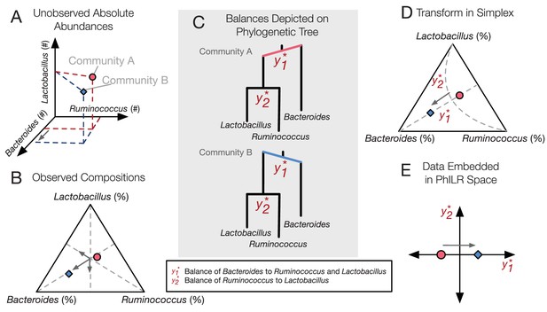
PhILR uses an evolutionary tree to transform microbiota data into an unconstrained coordinate system.
(A) Two hypothetical bacterial communities share identical absolute numbers of Lactobacillus, and Ruminococcus bacteria; they differ only in the absolute abundance of Bacteroides which is higher in community A (red circle) compared to community B (blue diamond). (B) A ternary plot depicts proportional data typically analyzed in a sequencing-based microbiota survey. Note that viewed in terms of proportions the space is constrained and the axes are not Cartesian. As a result, all three genera have changed in relative abundance between the two communities. (C) Schematic of the PhILR transform based on a phylogenetic sequential binary partition. The PhILR coordinates can be viewed as ‘balances’ between the weights (relative abundances) of the two subclades of a given internal node. In community B, the greater abundance of Bacteroides tips the balance to the right. (D) The PhILR transform can be viewed as a new coordinate system (grey dashed lines) in the proportional data space. (E) The data transformed to the PhILR space. Note that in contrast to the raw proportional data (B), the PhILR space only shows a change in the variable associated with Bacteroides.
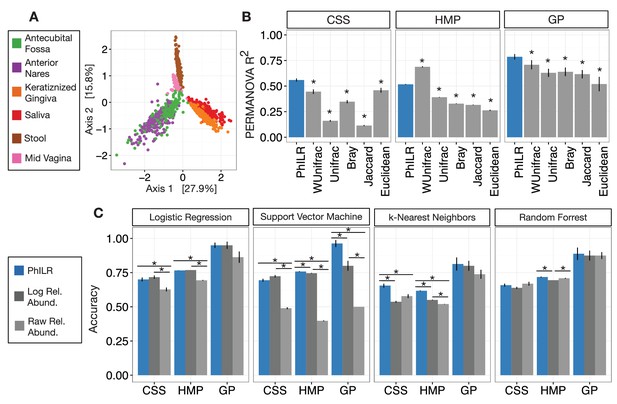
Performance of standard statistical models on PhILR transformed microbiota data.
Benchmarks were performed using three datasets: Costello Skin Sites (CSS), Global Patterns (GP), Human Microbiome Project (HMP) (a summary of these datasets after preprocessing is shown in Supplementary file 1 and Figure 2—figure supplement 1). (A) Sample distance visualized using principal coordinate analysis (PCoA) of Euclidean distances computed in PhILR coordinate system. A comparison to PCoAs calculated with other distance measures is shown in Figure 2—figure supplement 2. (B) Sample distance (or dissimilarity) was computed by a range of statistics. PERMANOVA R2 values, which represent how well sample identity explained the variability in sample pairwise distances, were used as a performance metric. Distances in the PhILR transformed space were calculated using Euclidean distance. Distances between samples on raw relative abundance data were computed using Weighted and Unweighted UniFrac (WUnifrac and Unifrac, respectively), Bray-Curtis, Binary Jaccard, and Euclidean distance. Error bars represent standard error measurements from 100 bootstrap replicates and (*) denotes a p-value of ≤0.01 after FDR correction of pairwise tests against PhILR. (C) Accuracy of supervised classification methods tested on benchmark datasets. Error bars represent standard error measurements from 10 test/train splits and (*) denotes a p-value of ≤0.01 after FDR correction of all pairwise tests.
-
Figure 2—source data 1
Source data for Figure 2b and c as well as FDR corrected p-values from tests.
- https://doi.org/10.7554/eLife.21887.004
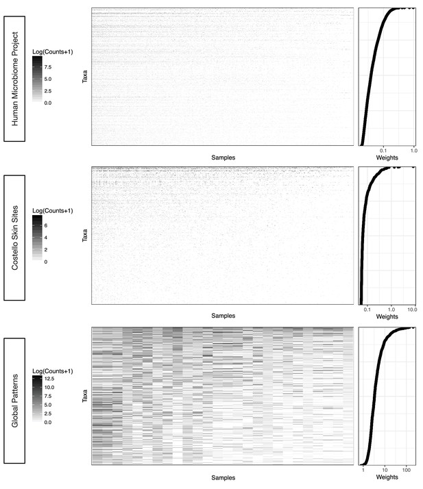
Taxa weighting scheme tends to assign smaller weights to taxa with more zero and near zero counts.
The weight of a given taxon is calculated as the geometric mean of its counts across all samples times the Euclidean norm of its relative abundance across all samples in the dataset (Materials and methods). Data are plotted on a log scale with a pseudocount of 1 added to ease visualization.
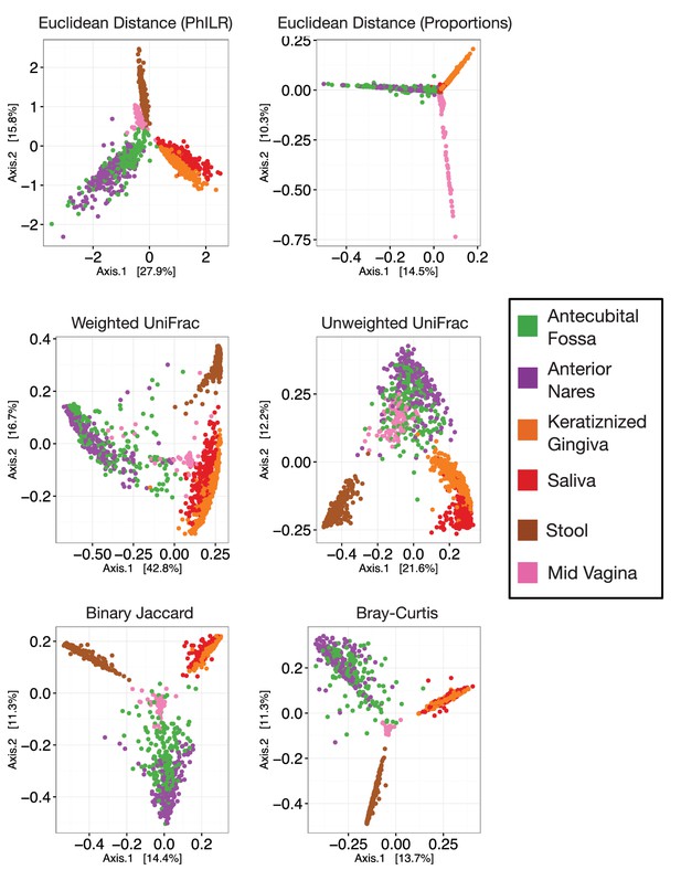
Principal coordinate analyses using different measures of community distance or dissimilarity.
https://doi.org/10.7554/eLife.21887.006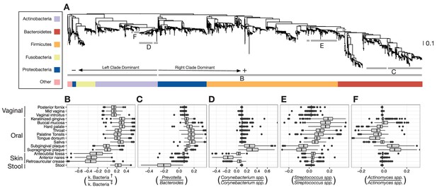
Balances distinguishing human microbiota by body site.
Sparse logistic regression was used to identify balances that best separated the different sampling sites (full list of balances provided in Figure 3—figure supplement 1). (A) Each balance is represented on the tree as a broken grey bar. The left portion of the bar identifies the clade in the denominator of the log-ratio, and the right portion identifies the clade in the numerator of the log-ratio. The branch leading from the Firmicutes to the Bacteroidetes has been rescaled to facilitate visualization. (B–F) The distribution of balance values across body sites. Vertical lines indicate median values, boxes represent interquartile ranges (IQR) and whiskers extend to 1.5 IQR on either side of the median. Balances between: (B) the phyla Actinobacteria and Fusobacteria versus the phyla Bacteroidetes, Firmicutes, and Proteobacteria distinguish stool and oral sites from skin sites; (C) Prevotella spp. and Bacteroides spp. distinguish stool from oral sites; (D) Corynebacterium spp. distinguish skin and oral sites; (E) Streptococcus spp. distinguish oral sites; and, (F) Actinomyces spp. distinguish oral plaques from other oral sites. (†) Includes Bacteroidetes, Firmicutes, Alpha-, Beta-, and Gamma-proteobacteria. (‡) Includes Actinobacteria, Fusobacteria, Epsilon-proteobacteria, Spirochaetes, and Verrucomicrobia.
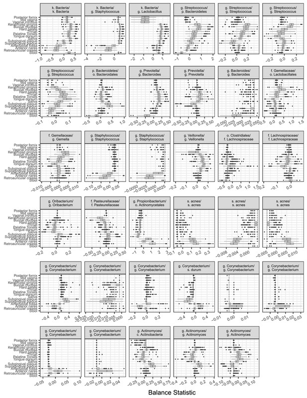
Balances found to distinguish human body sites by sparse logistic regression.
Taxa are listed in balance numerator/denominator format.
Neighboring clades covary less with increasing phylogenetic depth.
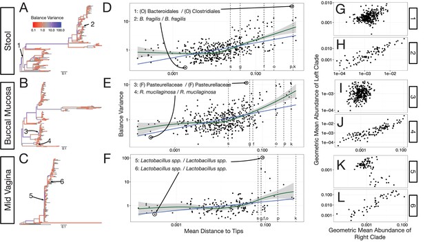
The variance of balance values captures the degree to which neighboring clades covary, with smaller balance variances representing sister clades that covary more strongly (Figure 4—figure supplement 1). (A–C) Balance variances were computed among samples from stool (A), buccal mucosa (B), and the mid-vagina (C). Red branches indicate small balance variance and blue branches indicate high balance variance. Balances 1–6 are individually tracked in panels (D–L). (D–F) Balance variances within each body site increased linearly with increasing phylogenetic depth on a log-scale (blue line; p<0.01, permutation test with FDR correction; Methods). Significant trends are seen across all other body sites (Figure 4—figure supplements 2 and 3). Non-parametric LOESS regression (green line and corresponding 95% confidence interval) reveals an inflection point in the relation between phylogenetic depth and balance variance. This inflection point appears below the estimated species level (‘s’ dotted line; the median depth beyond which balances no longer involve leaves sharing the same species assignment; Materials and methods). (G–L) Examples of balances with high and low variance from panels (A–F). Low balance variances (H, J, L) reflect a linear relationship between the geometric means of sister clades abundances. High balance variances (G, I, K) reflect either unlinked or exclusionary dynamics between the geometric means of sister clades abundances.
-
Figure 4—source code 1
Source code for Figure 4 and associated supplements.
- https://doi.org/10.7554/eLife.21887.010
-
Figure 4—source data 1
FDR corrected p-values from permutation tests.
- https://doi.org/10.7554/eLife.21887.011
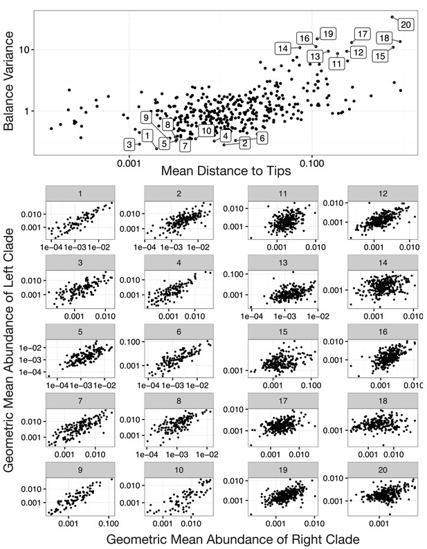
Balances with high and low variance.
Shown are the 10 highest and the 10 lowest variance balances for the Stool body site in the HMP dataset. Panels 1–10: Low balance variances reflect a linear relationship (through the origin) between levels of the two clades that descend from a given balance. Panels 11–20: High balances variances lack this linear relationship.
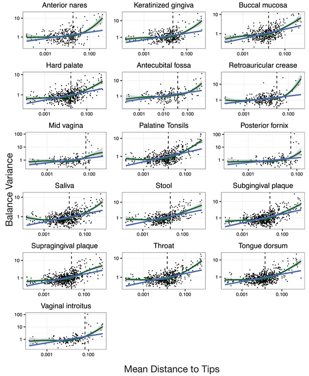
Neighboring clades covary less with increasing phylogenetic depth.
Shown here are all HMP body sites. Dotted lines indicate median species boundaries (see Materials and methods).
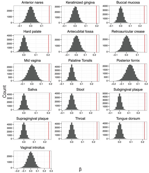
The null distribution for .
is the slope in the linear regression between balance variance and phylogenetic depth in log space (regressions shown in Figure 4—figure supplement 2). To form null distributions for , tip labels on the phylogeny were shuffled (n = 20,000) and balance values re-calculated. Distributions for are symmetric about 0 for each body site, suggesting.

Sign matrix representation of a phylogenetic tree.
A binary tree (Left) can be represented by a sign matrix (Right) denoted .
Additional files
-
Supplementary file 1
Extended benchmarking results including the effects of changing pseudocount and different choices for taxa and branch length weights.
This file also contains summary information for the benchmark datasets after preprocessing.
- https://doi.org/10.7554/eLife.21887.016
-
Supplementary file 2
Extended benchmarking results regarding the sensitivity of methods to different OTU filtering schemes.
- https://doi.org/10.7554/eLife.21887.017


