Cell lineage and cell cycling analyses of the 4d micromere using live imaging in the marine annelid Platynereis dumerilii
- Institut Jacques Monod, France
- Max Planck Institute of Molecular Cell Biology and Genetics, Germany
Figures
Figure 1 with 6 supplements
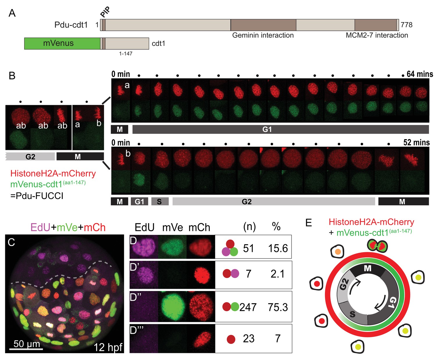
FUCCI cell cycle reporter for Platynereis dumerilii.
(A) P. dumerilii Cdt1 complete amino acid sequence above, showing the domains including PIP destruction box (N terminal). Below: a representation of the fused cell cycle construct containing mVenus fluorescent protein and a truncated part of Pdu-Cdt1. mVenus is a yellow fluorescent protein but is shown in green color for convenience throughout the manuscript. (B) Frames (every 4 min) from time-lapse (Figure 1—Video 1 and Figure 1—Video 2) showing division and cell cycling of an embryonic cell (labeled as ‘ab’) and its daughters (‘a’ and ‘b’). Fluorescent channels are shown separately for HistoneH2A-mCherry (red - nuclear) and mVenus-Cdt1(aa1-147) (green - cycling nuclear). The sister cells show significantly different cycling patterns, as indicated by bars marking the different cell cycle phases (M/G1/S/G2). (C) Example of an embryo which was injected with mRNA at two-cell stage, EdU-incubated for 3 min at 12hpf, and fixed immediately. The part below the dashed line is the injected side. All channels are merged. Red: Histone2A-mCherry; Green: mVenus-Cdt1(aa1-147); Magenta: EdU. (D–D’’’) Examples of cells that displayed different color combinations, and counts and percentages of cells based on data from six embryos (two independent experiments). (E) Cartoon summarizing the Pdu-FUCCI fluorescence patterns based on the time-lapse observations in B and EdU observations in D-D’’’.
Figure 1—figure supplement 1
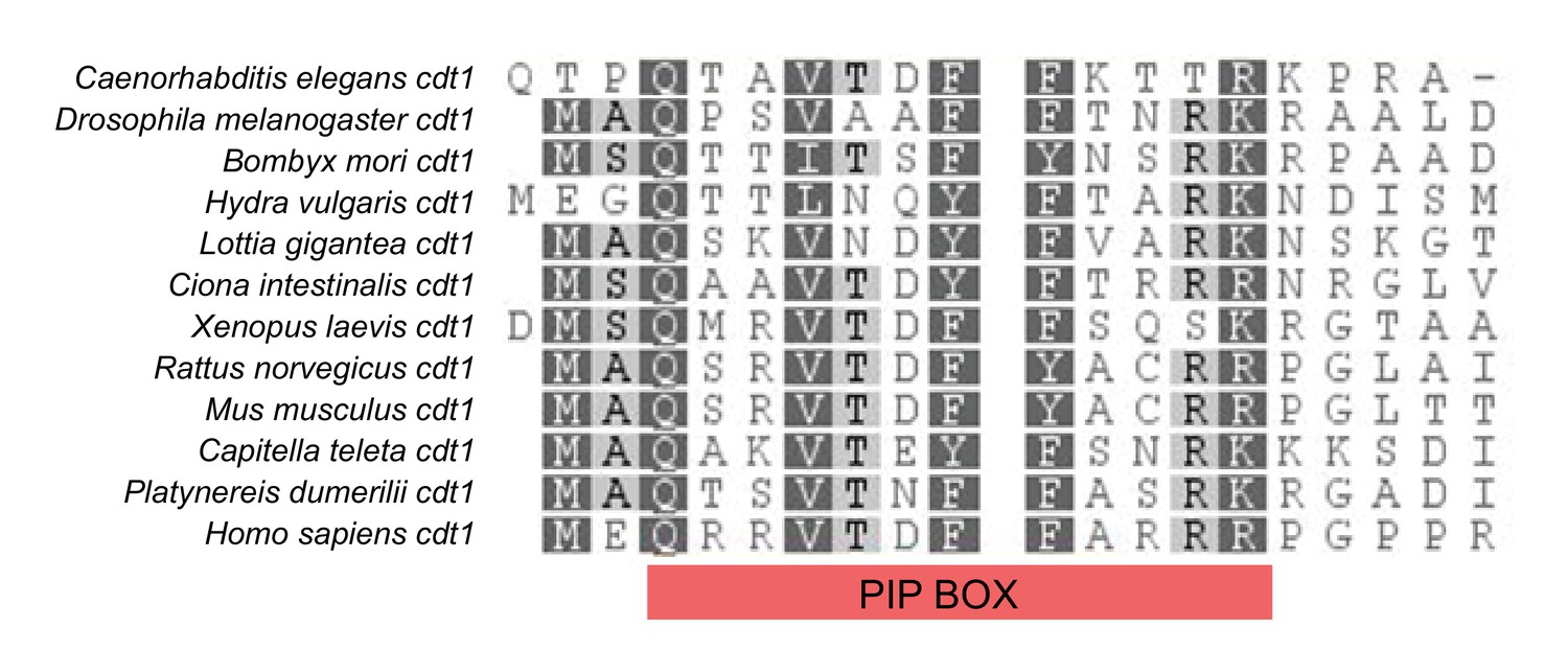
- Cdt1 amino acid alignments of destruction box sequences from different species.
Cdt1 amino acid alignment showing the region containing the PIP BOX (degron motif). The conserved motif for this degron in the human sequence is Q-x-x-[I/L/M/V]-T-D-[F/Y]-[F/Y]-x-x-x-[R/K]. We found a highly conserved region in the P. dumerilii sequence (aa3-14) corresponding to the PIP degron. For the cell cycle construct, a truncated (aa1-147) piece of Pdu-cdt1 sequence containing the PIP Box was used.
Figure 1—figure supplement 2
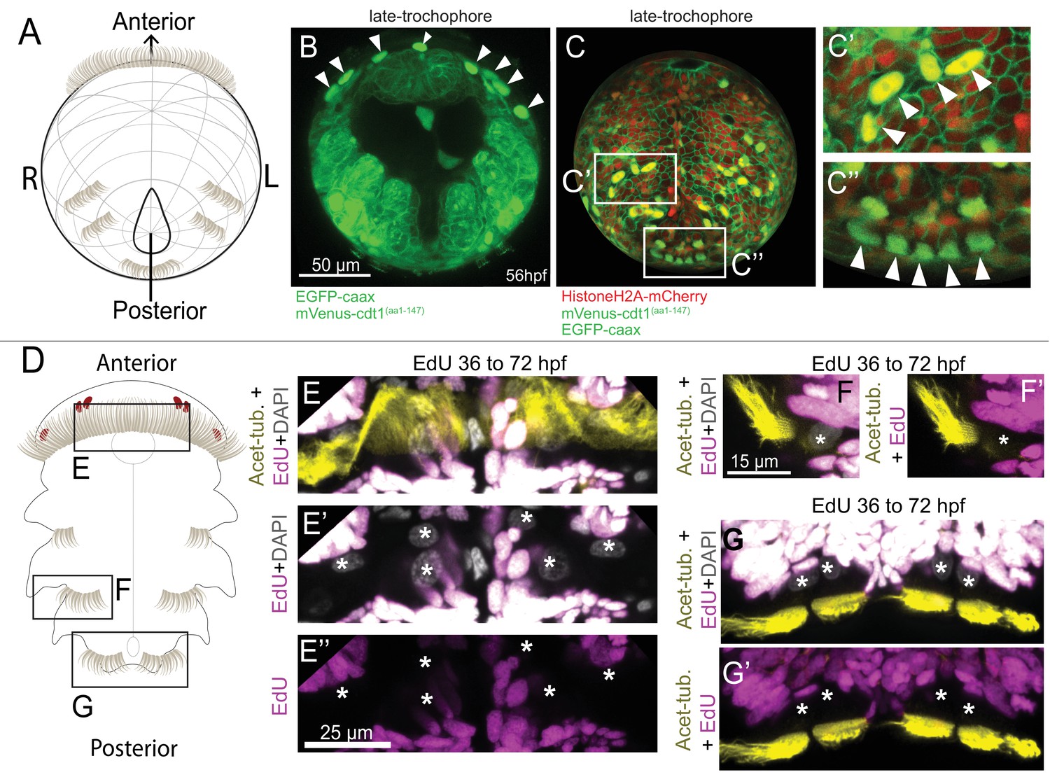
Multiciliated cells that exit the cell cycle can be visualized using Pdu-FUCCI.
(A) Cartoon of 48 hpf larva (ventral view), anterior up, slightly rotated up from the posterior end. (B–C’’) mVenus-Cdt1(aa1-147) (nuclear) and EGFP-caax (membrane) live-imaged together via single green channel. The orientation of sample in B is similar to cartoon in A. Strong mVenus signal persists in the nuclei of prototroch (arrowheads) (see Figure 1—Video 3 for earlier time points of the prototroch cells). (C) Ectoderm reconstruction of a larva injected with mVenus-cdt1(aa1-147), HistoneH2A-mCherry, and EGFP-caax mRNA (see Materials and methods and Figure 1—Video 4 for the ‘onionization’ process). The stage corresponds to late-trochophore stage. Paratroch cells show strong mVenus signal (arrowheads in C’ and C’’). (D) Cartoon of larva at 72 hpf, ventral view. Larvae were treated with EdU from 36 hpf until 72 hpf, and processed for immunohistochemistry (Acetylated-tubulin for cilia) and EdU reaction. Prototroch cells (E–E’’), and paratroch cells (F, G’) do not incorporate EdU after they are born confirming they have exited cell cycle and do not proceed to S phase. Stars indicate the troch cell nuclei.
Figure 1—video 1
Cell cycle reporter Pdu-FUCCI time-lapse in the early embryo (mCherry and mVenus).
The video shows an embryo injected with Histone2A-mCherry and mVenus-cdt1(aa1-147) mRNAs at one cell stage, imaged every 4 min, starting around 6:30 hpf for about 2 hr. The cells marked by arrowheads in the video (ab, a, b) are shown in detail in Figure 1B. Red: mCherry, Green: mVenus
Figure 1—video 2
Cell cycle reporter Pdu-FUCCI time-lapse in the early embryo (mVenus).
Same Figure 1—Video 1 is shown with mVenus (green) channel only.
Figure 1—video 3
Time-lapse of prototroch cells being born and exiting cell cycle.
Embryo was injected with Pdu-FUCCI (Histone2A-mCherry and mVenus-cdt1(aa1-147) and EGFP-caax mRNA at one-cell stage, and imaged every 10 min for about 6 hr. mVenus and EGFP signals are imaged from a single channel.
Figure 1—Video 4
Explanation of the onionization process, and display of all the onion layers.
Video is made from stack same as the sample shown in Figure 1—figure supplement 1C. Embryo was injected with Pdu-FUCCI and EGFP-caax mRNA at one-cell stage.
Figure 2
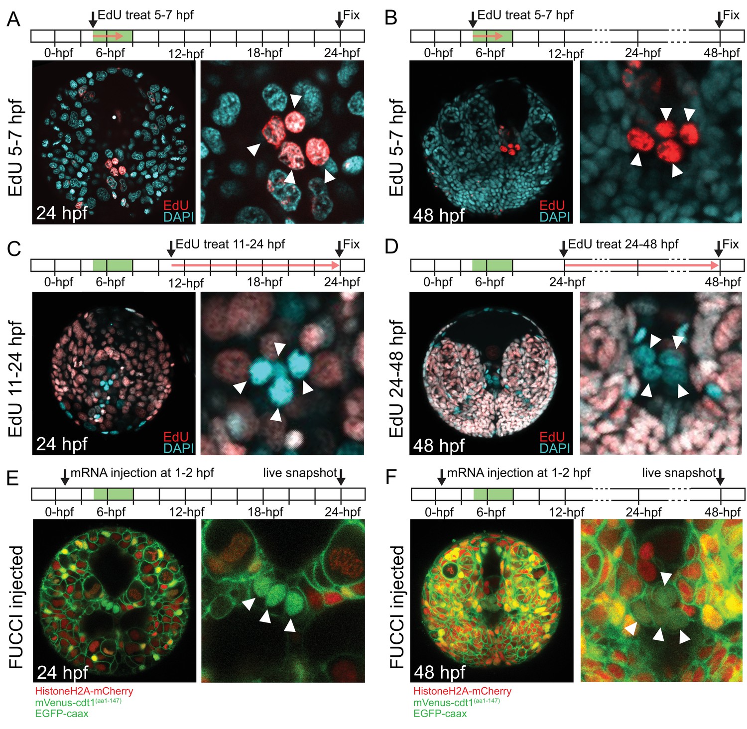
pPGCs do not incorporate EdU after they are born and retain mVenus-Cdt1(aa1-147) signal.
pPGCs (arrowheads) incorporate and retain the EdU signal (red) when treated during the time they are born (5–7 hpf), and can be easily detected at 24 hpf (A) or 48 hpf (B) due to retention of EdU. However, they do not incorporate EdU, if treated after they are born (C and D). Live samples that were injected with Pdu-FUCCI (HistoneH2A-mCherry, mVenus-cdt1(aa1-147)) and EGFP-caax and imaged at 24 hpf (E) and 48 hpf (F) show that pPGCs have the nuclear mVenus signal (green), also suggesting that they have stopped cycling (see also Figure 3, Figure 3—figure supplement 1, and Figure 7B). Green bars in the timeline schemas show the time period in which pPGCs are born. Red arrows in A–D show the period of EdU treatment. At least n = 6 samples were imaged for each EdU assay, and a representative sample is shown.
Figure 3 with 6 supplements
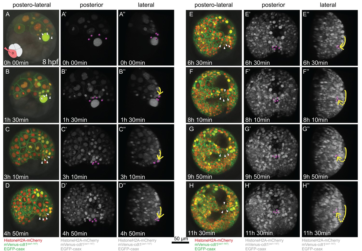
Time-lapse series of pPGC migration.
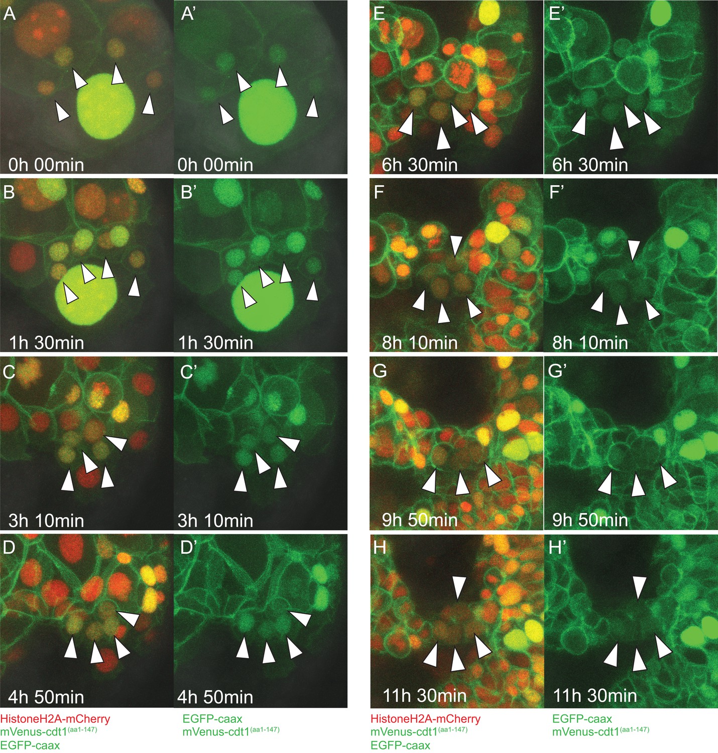
Embryo (Sample A) was injected with Pdu-FUCCI and EGFP-caax in the D quadrant and live-imaged with high time resolution (every 10 min). Time-lapse imaging started at 8 hpf and continued for 12 hr. Selected snapshots (elapsed time indicated on the lower-left corner) shown in the figure. (A–H) Z-projections from subsets of stacks showing the sample from a postero-lateral orientation, dorsal up, ventral down. pPGCs are indicated with arrowheads. (A’–H’) Same dataset analyzed in Imaris as Z-projection of full stacks, and rotated to a perfect posterior view in the software’s 3D viewer. All fluorescent signals are shown in grey color (set artificially in Imaris) and pPGCs (pink spots) were traced using the spots feature (Figure 3—video 3). (A’’–H’’) Lateral view of the same Imaris dataset, posterior to the right, dorsal up (Figure 3—video 4). Yellow arrow shows the approximate path of pPGCs as they migrate. Note that they travel on the surface (until E’’), then start assuming an internal position (indicated with the dashed yellow line) with the onset of epiboly. For the original video showing all time points and full-projection of stacks see Figure 3—video 1. For close-ups see Figure 3—figure supplement 1. (In the rest of the manuscript, this sample is analyzed for other developmental processes and is referred to as Sample A. Information from additional samples (Samples B and C) is provided in figure supplements.).
Figure 3—figure supplement 1
Close-ups of time-lapse video of pPGCs.
Close-ups of pPGCs for the frames from Figure 3—video 1 (Sample A) shown in Figure 3A–H are shown with merged fluorescent channels (A-H) and green fluorescent channel (A'-H') separately. Note that pPGCs (arrowheads) retain the nuclear mVenus signal throughout. Toward the end of the time-lapse, signal in pPGCs becomes weak and harder to see in these 3D-projections; however, measurements of nuclear signal show mVenus in pPGCs does not cycle (Figure 7B).
Figure 3—figure supplement 2
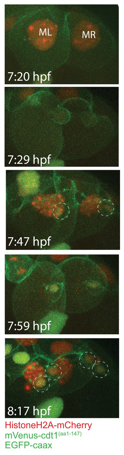
The first two divisions of ML and MR.
Frames showing the first two divisions of ML and MR, from a different sample injected with Pdu-FUCCI and EGFP-caax. Imaging started at 7:20hpf, done every 6 min, allowing to observe the first two divisions. These divisions give rise to the four pPGCs (dashed circles). pPGCs have both HistoneH2A-mCherry (red) and mVenus-Cdt1(aa1-147) (green) right after cell divisions are completed, indicated by the orange-green nucleus color.
Figure 3—video 1
Original 3D-projected time-lapse dataset with annotations (for Sample A).
Embryo was injected with Pdu-FUCCI and EGFP-caax mRNA into the D quadrant at four-cell stage, and imaged every 10 min. Note that uninjected side of the embryo appears dark. Also see Figure 5—video 1 and Figure 5—video 2 for additional samples imaged from a different batch of fertilization and injections.
Figure 3—video 2
Video of stack showing the same individual from Figure 3—video 1 imaged next day.
The sample displays normal development after injection and imaging.
Figure 3—video 3
pPGC migration traced in Imaris, posterior view.
Same confocal time-lapse dataset (Sample A) from Figure 3—video 1 was used for this analysis. Pink spots mark the pPGC nuclei.
Figure 3—video 4
pPGC migration traced in Imaris, lateral view
Same confocal time-lapse dataset (Sample A) from Figure 3—video 1 was used for this analysis. Pink spots mark the pPGC nuclei.
Figure 4 with 20 supplements
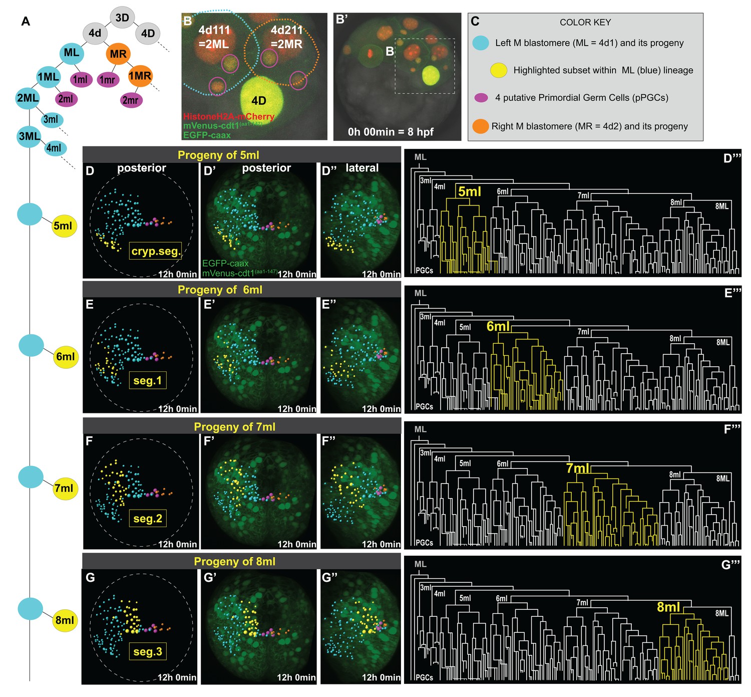
Primary blast cells give rise to clonal bocks of mesoderm.
The same sample as shown in Figure 3 (Sample A) was analyzed for mesodermal lineages in Bitplane Imaris. 4-cell stage embryo injected with Pdu-FUCCI (HistoneH2A-mCherry, mVenus-cdt1(aa1-147)) and EGFP-caax into D quadrant was live-imaged starting at 8 hpf every 10 min for 12 hr, from a posterior-lateral angle which enabled the tracing and visualization of the left mesoblast (ML = 4d1) lineage. Schema in A shows 4d lineage: ML (blue), MR (orange), pPGCs (pink), and highlighted subsets (yellow) are all color-coded (summarized in C) throughout this and following figures. Note that only a limited number of cells were traced for MR. Panel B (zoomed-in from B’) shows the starting frame of the time-lapse, and the position of ML and MR, with all three fluorescent constructs (see Figure 3—video 1 for the original time-lapse with annotations, and Figure 4—video 1 with spots for lineage tracing of ML). In the panels (D’- G’’), the last time point from this time-lapse (Sample A) is shown with EGFP-caax and mVenus-Cdt1(aa1-147) only (both in green), but HistoneH2A-mCherry (red) was removed for easier observation of the colored spots. 5ml lineage makes the mesoderm of the anterior-most left cryptic hemisegment (D–D’’’), 6ml makes the 1st larval left hemisegment (E–E’’’), 7ml the 2nd larval left hemisegment (F–F’’’), and 8ml the 3rd larval left hemisegment (G–G’’’). Panels D-G are the same orientation as D’-G’ but only showing the spots. D’–G’ show posterior orientation, and D’’-G’’ show lateral orientation. The lineages highlighted in yellow in D–G’’ are also shown in yellow in the lineage trees (D’’’–G’’’). See Figure 4—video 16 for an animated version of these lineages highlighted. Figure 4—video 2–13 show the full time-lapse of each lineage from posterior and lateral orientations, as well as 360-degree rotation.
Figure 4—figure supplement 1
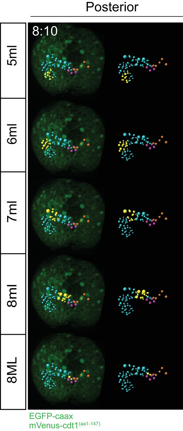
Progeny of each blast cell at an intermediate time point.
For a comparison to the final time point (12 hr 00 min) shown in Figure 4. Clonal domains (in yellow) of cells each primary blast cell gives rise to are already obvious at time point 8 hr 10 min. Blue: ML lineage, Yellow: subset highlighted within ML lineage, Pink: pPGCs, Orange: subset of MR lineage for reference.
Figure 4—figure supplement 2
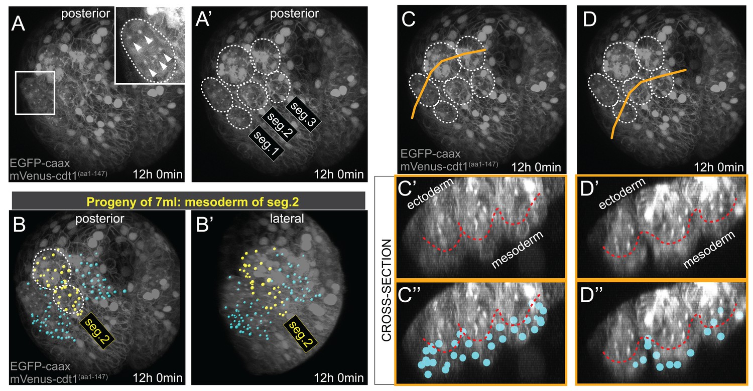
Mesodermal clonal clusters align with chaetal sacs specific to each hemisegment.
Chaetal sacs (ectodermal) are evident by the final time point (t = 72, or 12 hr 0 min) of the time-lapse (A–A’), which corresponds to about 37:35 hpf developmental time (Table 1). The chaetal sacs are often used as anatomical landmarks for determining larval segments, as there are two sacs per hemisegment (A’). The clonal mesodermal clusters (Imaris spots) align with the chaetal sacs of the relevant segment, an example for the second segment is shown in (B, B’), highlighted with yellow spot color. The spots are not ectodermal and do not overlap with the chaetal sacs, but instead lie beneath them at this stage (C–D’’). For obtaining cross sections in C’-D’’, the Imaris 3D stack with lineage spots at t = 72 was exported, and resliced in FIJI for visualizing cross-sections. Orange lines in C and D indicate the section planes shown in C’,C’’ and D’,D’’. Red dashed line marks the approximate border between the ectoderm (the chaetal sacs) and the mesoderm. Note that the spots marking the mesoderm are positioned mostly below the chaetal sacs (C’’,D’’), and those spots that overlap in these projections are located in-between the sacs.
Figure 4—figure supplement 3
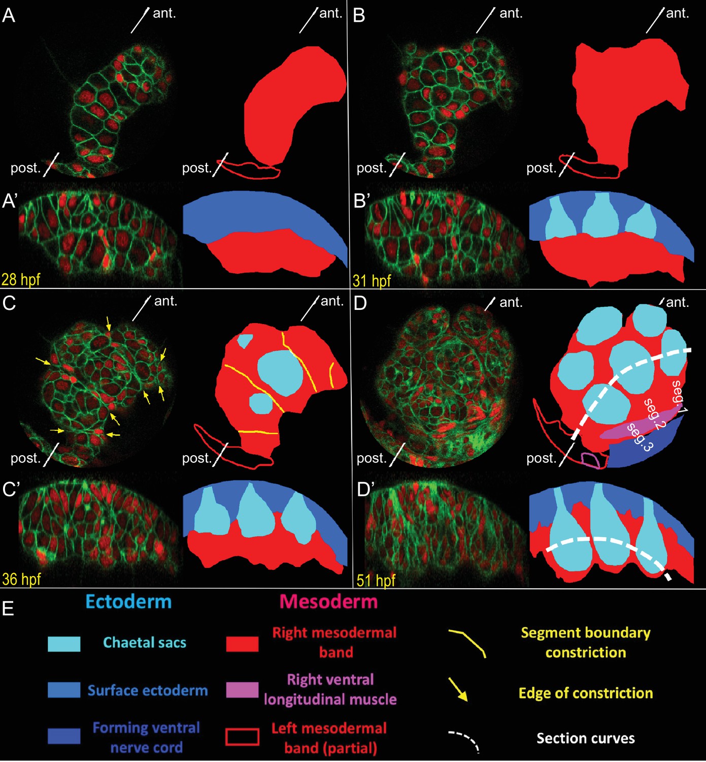
Live-imaging of the formation of mesodermal segmental blocks and the corresponding chaetal sacs.
Development of the right mesodermal band tissues, between the early trochophore and the late trochophore stages (from 26 hpf to 54 hpf) was time-lapse imaged (Figure 4—video 17). The embryo was injected in the D quadrant with HistoneH2A-mCherry (red) and EGFP-caax (green) mRNA, and was raised until swimming larva stage and imaged at a time resolution of every 67 min (18°C equivalent). Two visualizations of the same time point are shown in each panel: (i) an onion layer projection deep enough to exclude all surface ectoderm (A–D), and (ii) a curved section along the Z axis that follows the formation of the ventral row of chaetal sacs (A’–D’). An interpretation of the morphogenetic events is given with color code for each type of tissue. The position of section curves is indicated by white dashed lines (D, D’). At 28 hpf (A, A’), the mesodermal band is still a bean-shaped, rapidly proliferating block of tissue. At 31 hpf (B, B’), while the mesodermal band spreads dorso-ventrally, chaetal sacs start to form as pockets of ectodermal tissue above the mesodermal band. At 36 hpf (C, C’), the mesodermal band shows transient but very clear intersegmental constrictions possibly corresponding to segmental anlage. Note that this is about the same developmental point as shown in the last time point of the lineage-tracing dataset (Sample A) in the previous figures. Each segmental mesodermal block corresponds to one of the clonal blocks identified in the lineage tracing. Chaetal sacs elongate and each mesodermal block starts to surround a pair of chaetal sacs (C’). At 51 hpf (D, D’), the chaetal sacs are fully elongated and the mesoderm surrounds each one of them like a sheath. Note that approximate 18°C equivalents of developmental time in hours-post-fertilization (hpf) are shown in the panels.
Figure 4—video 1
Time-lapse of the ML lineage, and 360 rotation of the last time point.
Video shows spots from Imaris lineage tracing for extensively-traced ML lineage (blue), some tracing for MR lineage (orange), and pPGCs from both MR and ML (pink). Data set is the same as shown in Figure 3—video 1 (Sample A).
Figure 4—video 2
3ml, posterior view.
3ml sub-lineage is highlighted (yellow) within the ML lineage (blue) time-lapse video.
Figure 4—video 3
3ml, lateral view.
https://doi.org/10.7554/eLife.30463.024
Figure 4—video 4
4ml, posterior view.
4ml sub-lineage is highlighted (yellow) within the ML lineage (blue) time-lapse video.
Figure 4—video 5
4ml, lateral view.
https://doi.org/10.7554/eLife.30463.026
Figure 4—video 6
5ml, posterior view.
5ml sub-lineage is highlighted (yellow) within the ML lineage (blue) time-lapse video.
Figure 4—video 7
5ml, lateral view.
https://doi.org/10.7554/eLife.30463.028
Figure 4—video 8
6ml, posterior view.
6ml sub-lineage is highlighted (yellow) within the ML lineage (blue) time-lapse video.
Figure 4—video 9
6ml, lateral view.
https://doi.org/10.7554/eLife.30463.030
Figure 4—video 10
7ml, posterior view.
7ml sub-lineage is highlighted (yellow) within the ML lineage (blue) time-lapse video.
Figure 4—video 11
7ml, lateral view.
https://doi.org/10.7554/eLife.30463.032
Figure 4—video 12
8ml, posterior view.
8ml sub-lineage is highlighted (yellow) within the ML lineage (blue) time-lapse video.
Figure 4—video 13
8ml, lateral view.
https://doi.org/10.7554/eLife.30463.034
Figure 4—video 14
8ML, posterior view.
8ML sub-lineage is highlighted (yellow) within the ML lineage (blue) time-lapse video.
Figure 4—video 15
8ML, lateral view.
https://doi.org/10.7554/eLife.30463.036
Figure 4—video 16
Animation of the segmental mesoderm clonal regions.
Posterior and lateral views together.
Figure 4—video 17
Segment formation in the P. dumerilii larva.
Embryo was injected with HistoneH2A-mCherry and EGFP-caax mRNA, raised until 24 hpf swimming larval stage, immobilized with DMSO treatment and mounted in low-melting agarose for time-lapse live-imaging. The resulting 4D dataset was modified in FIJI with the Onionizer (see Materials and methods) to reveal the curved ectodermal and mesodermal larval segments forming. Upper row is the lateral view, middle row is the cross-section, and lower row is the label key with corresponding colors. The timer shows the calculated developmental time. See Figure 4—figure supplement 3 for details.
Figure 5 with 3 supplements
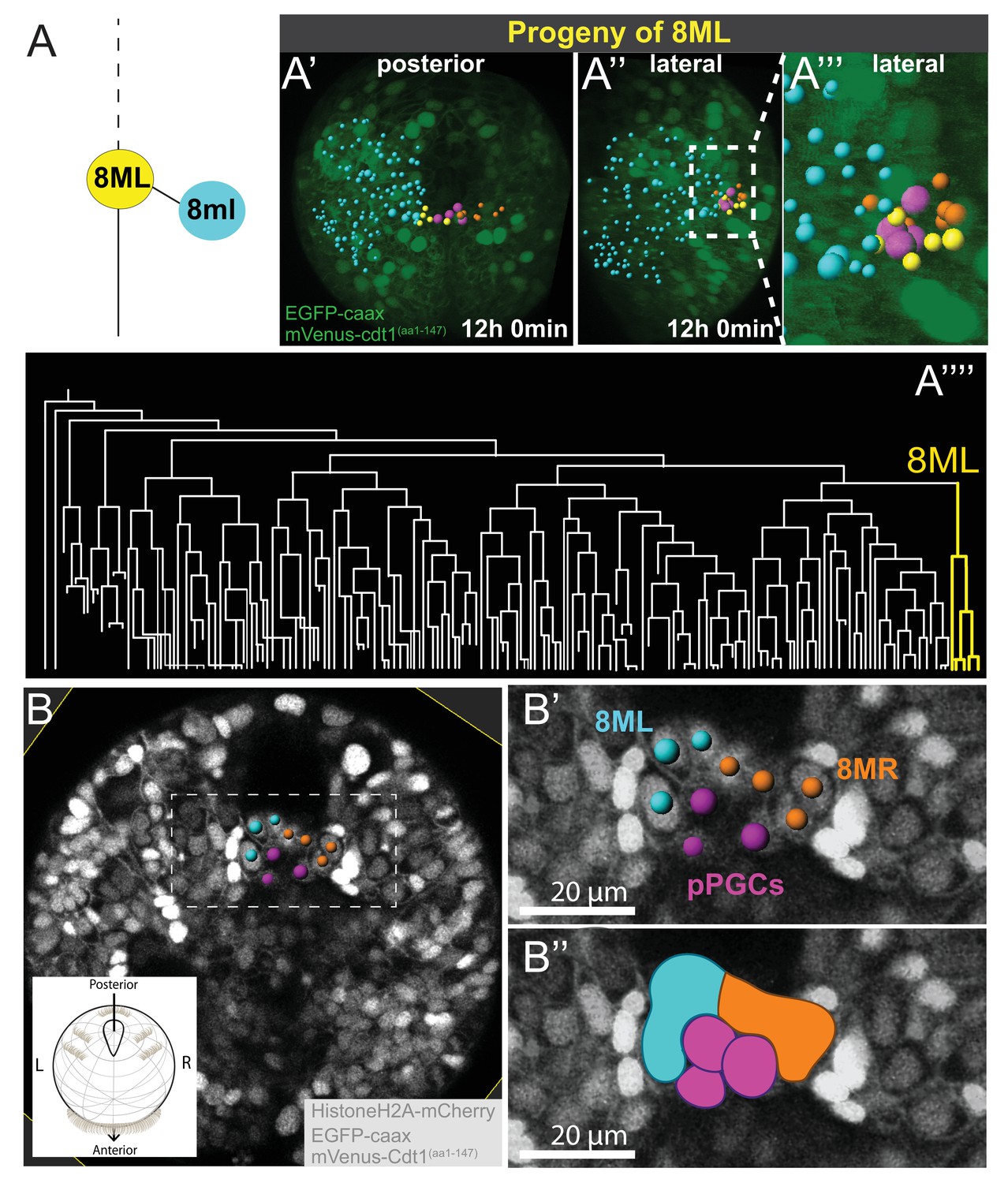
8ML/R give rise to the mesodermal posterior growth zone.
Continuation of lineage analysis (in Figure 4) of Sample A shows that (A) the 8ML cell created during the 8th division gives rise to a few cells near the pPGCs (A’–A’’), where the mesodermal posterior growth zone is located. The 8ML lineage is highlighted in the tree (A’’’). Another sample (Sample B) with different orientation is shown in B-B’’. A subset of 3D-projected focal planes show how the 8ML/8MR lineages are located immediately posterior to the pPGCs (B’, B’’). The same color coding as in Figure 4 is used: Blue is ML lineage, orange is MR, pink is pPGCs, and yellow 8ML. For a comparison of three different samples with 8ML/MR lineages traced see Figure 5—figure supplement 1. See Figure 4—video 14 and Figure 4—video 15 for full time-lapse with spots showing lineages, from posterior and lateral orientations, as well as 360˚ rotation (Figure 4—video 14). All signals from fluorescent constructs is shown in green (EGFP-caax and mVenus-Cdt1(aa1-147), in A’-A’’’) or in grayscale (Histone2A-mCherry, EGFP-caax, and mVenus-Cdt1(aa1-147)) to highlight general morphology.
Figure 5—figure supplement 1
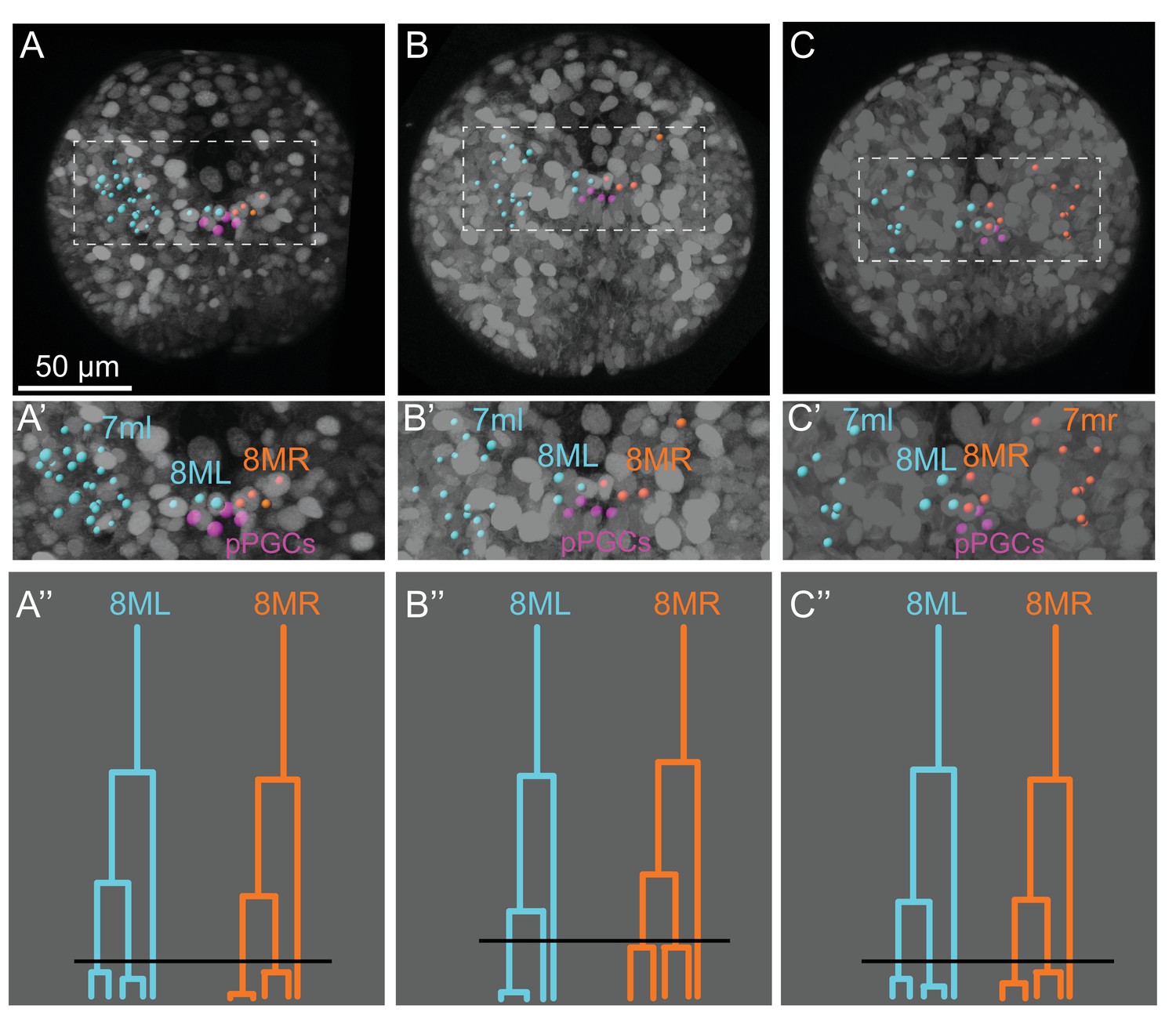
Cell lineages from additional samples compared with the sample shown in the main text.
For easier comparison, only some cell lineages in ML and MR are highlighted in each sample. Sample A is the one shown in the main text (A). Samples B and C were partially traced for confirming lineages (B, C). In all three samples, 7ml gives rise to mesodermal cells located on the left side of the 2nd larval segment (A’, B’, C’). 7mr was observed to make a symmetric region to 7ml on the right (only analyzed in the third sample (C, C’). Similarly, 8ML and 8MR gave rise to lineages located near pPGCs (in pink), and lineage trees of all three samples for these cells look very similar. Black lines in (A’’, B’’, C’’) indicate the time point shown in snapshots in (A, B, C). These time points were chosen for comparison of each sample at an equivalent time point where both 8ML and 8MR has given rise to 3 cells each, and some of these cells are about to divide. B’ shows nuclei position by spots while B’’ shows cell delineations indicating direct contact between pPGCs and MPGZ cells. All fluorescence signals from Pdu-FUCCI (HistoneH2A-mCherry, mVenus-Cdt1(aa1-147)) and EGFP-caax are shown in grayscale.
Figure 5—video 1
Time-lapse of Sample B.
Video shows time-lapse 3D projections of Sample B, imaged every 12 mins for 13 hr. Embryo was injected with Pdu-FUCCI and EGFP-caax mRNA into the D quadrant at four-cell stage.
Figure 5—video 2
Time-lapse of Sample C.
Video shows time-lapse 3D projections of Sample C, imaged every 12 mins for 13 hr. Embryo was injected with Pdu-FUCCI and EGFP-caax mRNA into the D quadrant at four-cell stage.
Figure 6
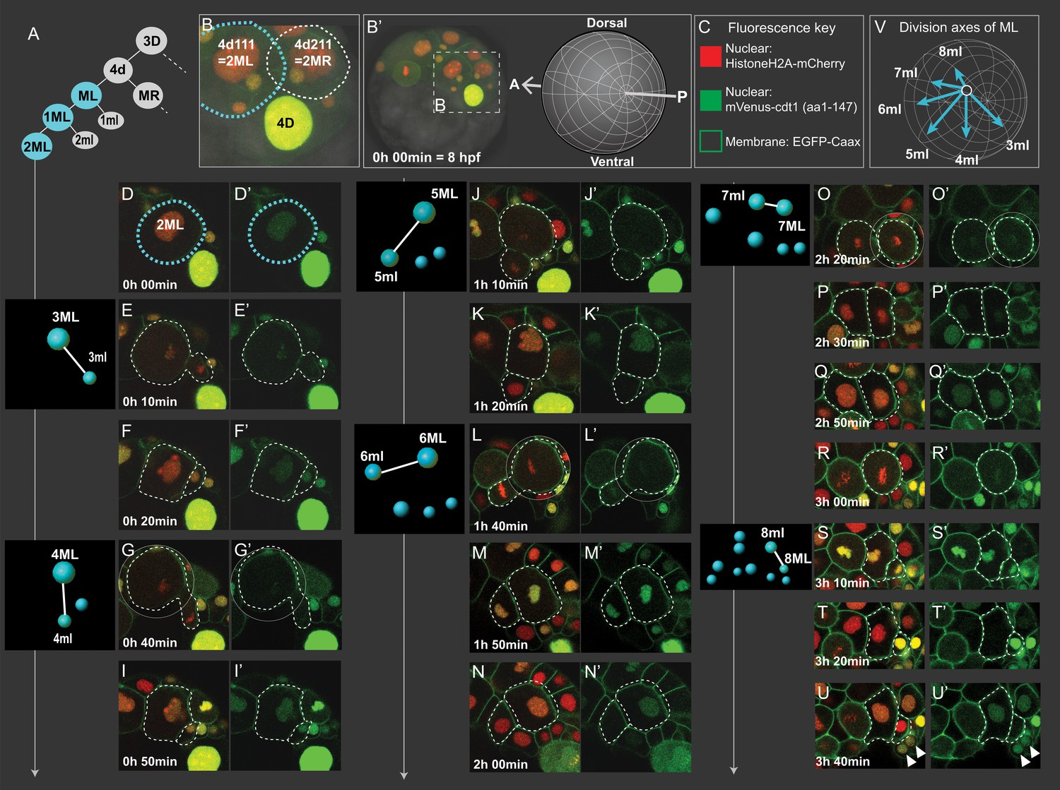
Cell divisions of 4d lineage giving rise to the mesodermal primary blast cells.
Same dataset shown in Figures 4 and 5 (Sample A) was analyzed for cell division size asymmetry and orientation. In (A), schema shows the 4d lineage divisions, ML in blue. The spot diagrams next to the images show the division by which each primary blast cell is created. The direction of division shown in spot diagrams represents the actual division axis. (B) is a zoomed-in panel from (B’) showing the mesoblasts after two rounds of division (2ML = 4d111, and 2MR = 4d211). The orientation of imaging is depicted in (B’). In (C), fluorescence key shows the color and location of each construct. Throughout D-U (merged channels) and D'-U' (green channel only) snapshots of ML’s divisions from the live imaging dataset are shown, outlined with dashed lines. Note that the initial divisions are highly asymmetric in size (E, G, J, L, S) while the division that creates 7ml and 7ML appears symmetric (O). In V, the division axes for all primary blast cells are shown together. See Figure 3—video 1 for the time-lapse dataset, the snapshots are derived from (Sample A). Arrowheads in (U, U’): pPGCs. Time is shown as elapsed imaging time (Table 1).
Figure 7 with 2 supplements
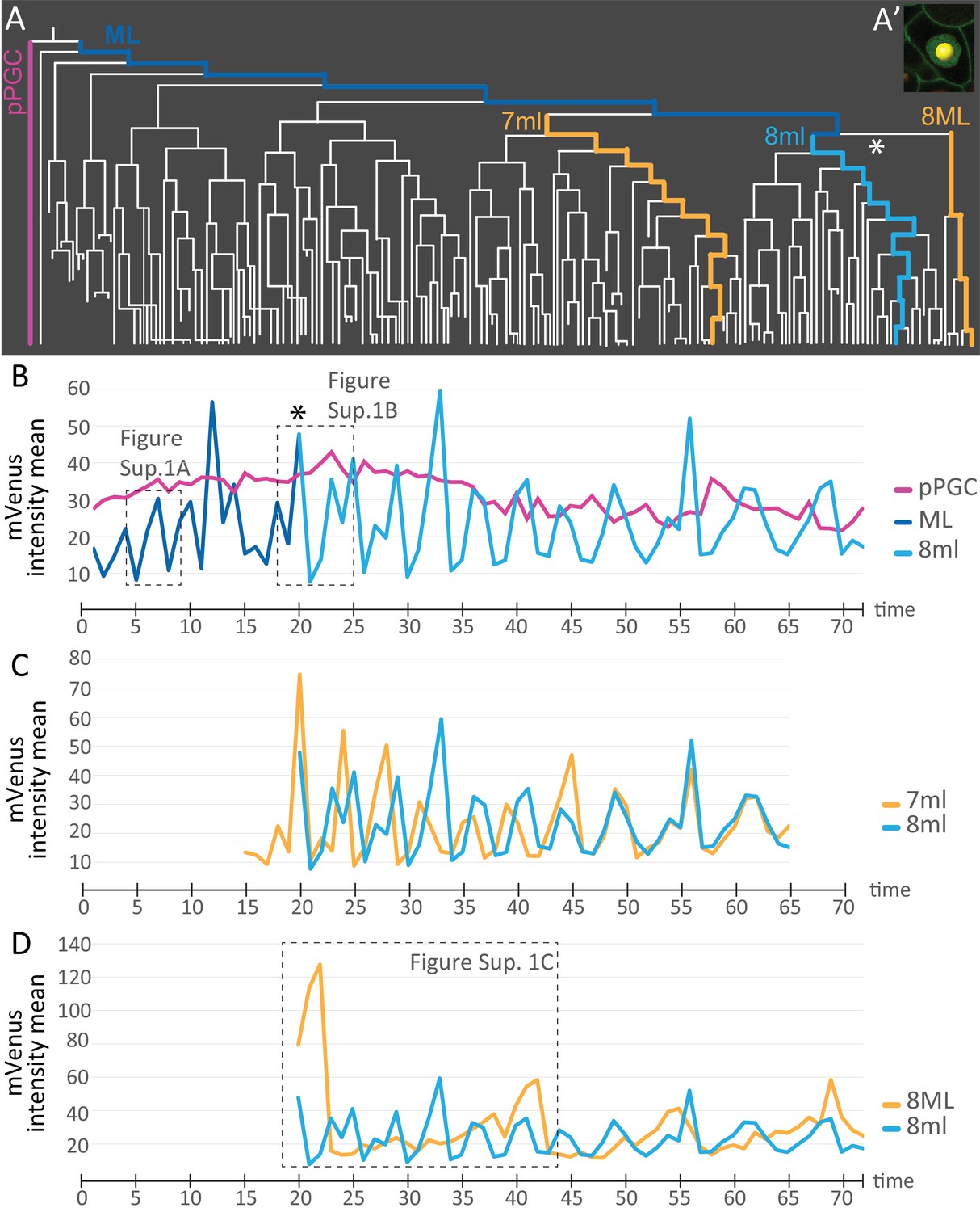
Comparison of mVenus-Cdt1(aa1-147) intensity across different cell lineages.
(A) The lineages selected for cell cycle signature analysis are indicated in color (matching the colors used in the subsequent graphs). (A’) Example of a spot placed in the middle of the nuclear signal (only one focal plane from the stack shown here), and used for obtaining ‘mVenus fluorescence intensity mean’ measurements for each nucleus per time point in Imaris. (B) Comparison of mVenus intensity across 3 cell lineages. 8ml (light blue) is plotted as a continuation of the mesoblast ML (dark blue). Star indicates the time point 7ML divides into 8ml and 8ML in the lineage tree (A) and the cell cycle graph (B). (C) Two lineages from 7ml and 8ml show similar cycling patterns. Despite being slightly out of phase at the beginning, they become synchronized around time point 46. (D) Same 8ml lineage is compared this time with a lineage from 8ML, which is the lineage that gives rise to the mesodermal posterior growth zone cells, and is much slower in its cycling. In B and D, the dashed boxes show the excerpts from the graphs analyzed in Figure 7—figure supplement 1. Time axis shows time points (Table 1). Fluorescence measurement is in arbitrary units (Figure 7—source data 1).
-
Figure 7—source data 1
- https://doi.org/10.7554/eLife.30463.047
Figure 7—figure supplement 1
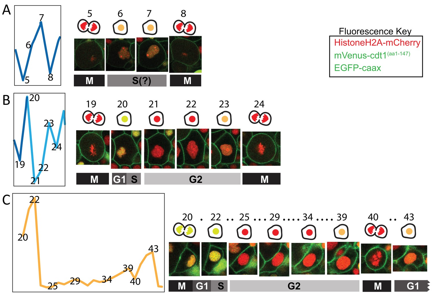
Details from the cell cycle graphs.
Excerpts from the cell cycle graphs presented in Figure 7 are shown here with snapshots of the cell nuclei corresponding to the time points on the graphs (indicated as matching numbers on the graphs and above the images). The cartoons above cell snapshots show simplified versions of those cells, with nuclei color matching the fluorescent signal. Red: mCherry only; Yellow: mCherry + mVenus; Orange: mCherry + lower mVenus. Dots in C indicate time points not shown here. M: Mitosis, G1: Gap phase 1, S: Synthesis, G2: Gap phase 2. Fluorescent protein colors are indicated in the ‘Fluorescence Key’ box.
Figure 7—figure supplement 2
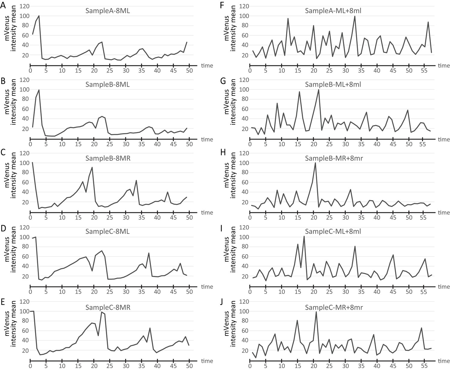
Cell cycle graphs compared across different live-imaged samples.
Sample A is the sample shown in the main figures in the manuscript. Cell cycle graphs obtained from the same cell lineages from two additional time-lapse samples (Samples B and C) are compared with Sample A. The volume of mRNA injected in each sample slightly differs leading to differences in the measured intensity of fluorescence. For easier comparison, data were normalized by finding the maximum for each series, dividing all time points by the maximum, and multiplying by 100. The same letter codes are used for the samples as in Figure 5—figure supplement 1. Cell lineages show very similar cycling patterns in all samples (A-E show 8ML and 8MR from different samples; (F–J) show ML +8ml from different samples) (Figure 7—source data 1).
Figure 8

ML lineage tree indicating known and novel sub-lineages in P. dumerilii, and comparison of P. dumerilii with the leech.
Lineage tree of cells that arise from the left mesoblast (ML) traced in Imaris is plotted in A. Colors show the extent of lineage analyses accomplished in earlier studies. The same lineage tree is shown in A’ with color-coded sub-lineages for each primary blast cell, pPGCs, and 8ML. The same color codes are used in the Platynereis larva cartoon in B. On the left in B, 4d lineage diagram is shown with primary blast cells labeled with the mesodermal region they contribute to. Note how the cells from the first two divisions of ML (pPGCs) end up next to the cells in the mesodermal posterior growth zone (MPGZ), which are born much later. For comparison, 4d (DM’’) lineage diagram and primary blast cell lineages (again color-coded) are shown in C for the leech (a clitellate annelid) (Cho et al., 2014; Gline et al., 2011; Rebscher, 2014). The first six divisions of ML make cells that contribute to non-segmental mesoderm in anterior regions and the gut (both in dark gray). The following divisions make segmental primary blast cells, each or which contributes to the mesoderm of two consecutive hemisegments (for example, sm1 contributes to part of first segment and part of second segment mesoderm, in total making one segment-worth of mesoderm). Note that in the leech, PGCs (pink) arise in later cell divisions, as a subset within the segmental mesoderm population that originate from a primary blast cell (sm10, and sm12 through 22).
Figure 9

Phylogenetic distribution of embryonic and post-embryonic teloblasts in some annelids, and the relation to the number of segments made.
A simplified annelid phylogeny (Weigert and Bleidorn, 2016) summarizes the main annelid species investigated for segment formation and teloblasts. The number of segments appearing during the pelagic larval phase (but patterned during embryogenesis) and the number of segments added posteriorly after the start of benthic life can vary considerably (Balavoine, 2014). In leeches, a fixed number of segments is made during direct embryonic development and none added after hatching. In non-leech clitellates (such as Tubifex), the embryos make a few tens of segments during embryogenesis and add many more after hatching. In non-clitellate annelids (Errantia, Sedentaria, and early branching), the number of larval segments is variable, and many more are added in post-larval development: In Nereidids (Errantia) such as Platynereis, only three larval segments develop, while in Capitella (Sedentaria), 13 larval segments (Thamm and Seaver, 2008) and in Chaetopterus (an early-branching annelid) 15 larval segments develop (Seaver et al., 2001). Embryonic and post-embryonic teloblasts differ in the way they have been evidenced. Embryonic teloblasts in the Clitellates (Weisblat and Kuo, 2014; Goto et al., 1999a; Nakamoto et al., 2011) and in Platynereis (this work) have been directly observed in live specimens. By contrast, post-embryonic teloblasts are inconspicuous cells that are identified only so far by their molecular stem cell signature (Gazave et al., 2013; Dill and Seaver, 2008; Özpolat et al., 2016). No direct observation of post-embryonic teloblast patterns of division is available so far. No direct evidence for embryonic teloblasts giving birth to post-embryonic teloblasts exists in any species so far to our knowledge. The ancestor of annelids presumably had both larval and post-larval segments, and thus it raises the question of the presence of both embryonic and post-embryonic teloblasts in this ancestral annelid, and even more broadly in other spiralians such as chitons (a type of segmented mollusk). Structures shown in the figure are color coded and explained in the ‘symbol key’.
Figure 10 with 1 supplement
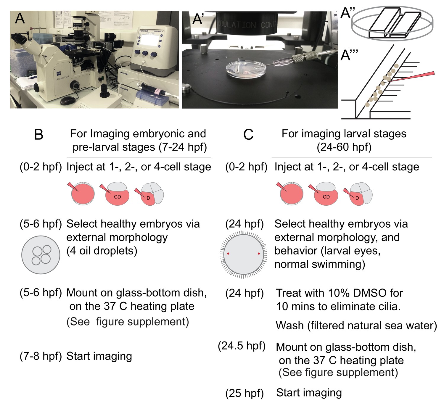
Injection setup and general experimental outline for imaging samples.
(A) A Zeiss inverted scope with a gliding stage, coupled with the Eppendorf Femtojet microinjector and Eppendorf Transferman micromanipulation system were used for injections. Femtotip ready-to-use injection needles were back-filled with injection solution (A’). An agarose platform (A’’) with a groove large enough to contain embryos was prepared using a plastic custom-made mold. Under a dissecting scope, small incisions were made to the right side of the groove (A’’’), and these incisions were used to remove embryos from the needle by sliding the needle through them. The agarose platform was placed into a small petri dish lid and covered with filtered sea water before the embryos were transferred into the dish. In B and C, the steps of general experimental outline for live imaging samples at different stages are listed.
Figure 10—figure supplement 1
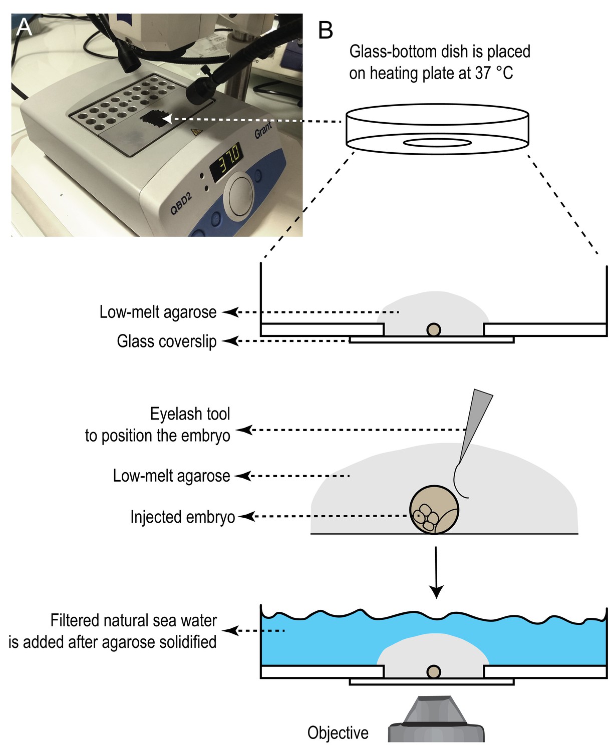
Heating plate setup for mounting samples in glass-bottom dishes.
A) One of the heating blocks was turned upside down to use its flat surface, and was painted with black marker to provide contrasting background for mounting samples. The heating plate was placed under a stereoscope. Temperature was set to 37˚C. B) Glass-bottom dishes were pre-warmed on this surface. One injected sample was placed on the dish with as little sea water as possible. Next, a drop of 100 µl of 1% low-melting agarose was added on, and before the agarose started solidifying, the sample was rotated to the desired position with the help of an eyelash tool. If needed, more agarose was slowly added with the help of a micropipette to cover the glass surface completely. Then the plate was transferred on a colder surface to let agarose solidify. Once agarose solidified (in about 3–5 min), filtered natural sea water was added on top to cover the agarose, and the dishes were covered with the lid and kept at 18˚C incubator, in a wet chamber, until imaging.
Tables
Table 1
Calculated developmental time and corresponding stage for each time point at imaging temperatures.
For the video (Sample A) from which we show most of the lineage tracing data in this manuscript, we calculated what each time point roughly corresponds to in the normal staging by Fischer et al., 2010. This calculation was done based on the starting stage, end stage, and how long this normally takes under 18˚C conditions. For example, Figure 3—video 1 (used in Figures 3, 4, 5 and 6) starts at eight hpf (stereoblastula stage), and in the final time point the sample appears towards the end of mid trochophore stage. Even though elapsed time is 12 hr of imaging (72 time points), under 18˚C incubation conditions, about 35–40 hr is required to reach this stage. Thus, we calculated each time point in the live-image dataset corresponding roughly to: T = 8 hr + (25mins x tp), where ‘tp’ is time point, and T is the calculated developmental time. According to this, the end calculated developmental time for Figure 3—video 1 is: T = 8 hr + (25 mins x 72)=37 hr 35 min.
| Time point (tp) | Elapsed imaging time (hr:min:s) | Calculated developmental time (T) at 18˚C (hr:min:s) | Corresponding developmental stage at 18˚C (Fischer et al., 2010) |
|---|---|---|---|
| 1 | 0:00:00 | 8:00:00 | Stereoblastula |
| 3 | 0:20:00 | 8:50:00 | Stereoblastula |
| 5 | 0:40:00 | 9:40:00 | Stereoblastula |
| 7 | 1:00:00 | 10:30:00 | Stereoblastula |
| 9 | 1:20:00 | 11:20:00 | Stereoblastula |
| 11 | 1:40:00 | 12:10:00 | Stereoblastula |
| 13 | 2:00:00 | 13:00:00 | Protrochophore |
| 15 | 2:20:00 | 13:50:00 | Protrochophore |
| 17 | 2:40:00 | 14:40:00 | Protrochophore |
| 19 | 3:00:00 | 15:30:00 | Protrochophore |
| 21 | 3:20:00 | 16:20:00 | Protrochophore |
| 23 | 3:40:00 | 17:10:00 | Protrochophore |
| 25 | 4:00:00 | 18:00:00 | Protrochophore |
| 27 | 4:20:00 | 18:50:00 | Protrochophore |
| 29 | 4:40:00 | 19:40:00 | Protrochophore |
| 31 | 5:00:00 | 20:30:00 | Protrochophore |
| 33 | 5:20:00 | 21:20:00 | Protrochophore |
| 35 | 5:40:00 | 22:10:00 | Protrochophore |
| 37 | 6:00:00 | 23:00:00 | Protrochophore |
| 39 | 6:20:00 | 23:50:00 | Protrochophore |
| 41 | 6:40:00 | 24:40:00 | Early trochophore |
| 43 | 7:00:00 | 25:30:00 | Early trochophore |
| 45 | 7:20:00 | 26:20:00 | Mid-trochophore |
| 47 | 7:40:00 | 27:10:00 | Mid-trochophore |
| 49 | 8:00:00 | 28:00:00 | Mid-trochophore |
| 51 | 8:20:00 | 28:50:00 | Mid-trochophore |
| 53 | 8:40:00 | 29:40:00 | Mid-trochophore |
| 55 | 9:00:00 | 30:30:00 | Mid-trochophore |
| 57 | 9:20:00 | 31:20:00 | Mid-trochophore |
| 59 | 9:40:00 | 32:10:00 | Mid-trochophore |
| 61 | 10:00:00 | 33:00:00 | Mid-trochophore |
| 63 | 10:20:00 | 33:50:00 | Mid-trochophore |
| 65 | 10:40:00 | 34:40:00 | Mid-trochophore |
| 67 | 11:00:00 | 35:30:00 | Mid-trochophore |
| 69 | 11:20:00 | 36:20:00 | Mid-trochophore |
| 71 | 11:40:00 | 37:10:00 | Mid-trochophore |
| 72 | 11:50:00 | 37:35:00 | Mid-trochophore |
Key resources table
| Reagent type (species) or resource | Designation | Source or reference | Identifiers | Additional information |
|---|---|---|---|---|
| Gene (Platynereis dumerilii) | Pdu-cdt1 | NA | GenBank No: MF614951 | From the full 2337 bp coding sequence, a 1946 bp part including the start site, and ending before the stop codon was amplified |
| Strain, strain background (P. dumerilii) | Wild Type | Institut Jacques Monod cultures | ||
| Recombinant DNA reagent | pCS2+ mVenus-cdt1(aa1-147) | this paper | GenBank No: MF614950 | |
| Recombinant DNA reagent | pEXPTol2-H2A-mCherry | Other | Plasmid was not specifically produced for this paper, and has been published before. The source plasmids used for the constructions of this plasmid was provided by Caren Norden Lab (MPI-CBG, Dresden, Germany). | |
| Recombinant DNA reagent | pEXPTol2-EGFP-CAAX | Other | Plasmid was not specifically produced for this paper, and has been published before. The source plasmids used for the constructions of this plasmid was provided by Caren Norden Lab (MPI-CBG, Dresden, Germany). | |
| Antibody | Acetylated-tubulin | Sigma-Aldrich | T7451, RRID:AB_609894 | (1:500) |
| Sequence-based reagent | Pdu-cdt1- Forward Primer | this paper | TTGTTTTCTTGTTGAGGTGGGATG | |
| Sequence-based reagent | Pdu-cdt1- Reverse Primer | this paper | GGAGATGACGAGACAGGCAG | |
| Sequence-based reagent | pCS2+ vector backbone – Forward Primer | this paper | CTAGAACTATAGTGTGTTGTATTACGT | |
| Sequence-based reagent | pCS2+ vector backbone – Reverse Primer | this paper | AGAGGCCTTGAATTCGAATCG | |
| Commercial assay or kit | Gibson assembly master mix | NEB France | E2611S | |
| Commercial assay or kit | Click-iT EdU Alexa Fluor 647 Imaging Kit | Life Technologies | C10340 | |
| Commercial assay or kit | SP6 mMessage kit | Ambion, ThermoFisher | AM1340 | |
| Commercial assay or kit | MEGAclear kit | Ambion, ThermoFisher | AM1908 | RNA elution option two with the modifications - see Materials and methods for details |
| Commercial assay or kit | Proteinase K | Ambion, ThermoFisher | AM2548 | 20 µg/µl final concentration |
| Software, algorithm | Bitplane Imaris (Version 8.2) | |||
| Software, algorithm | Onionizer | https://figshare.com/s/1c0dcd120d13deb888ba |
Additional files
-
Transparent reporting form
- https://doi.org/10.7554/eLife.30463.052
Download links
A two-part list of links to download the article, or parts of the article, in various formats.
Downloads (link to download the article as PDF)
Open citations (links to open the citations from this article in various online reference manager services)
Cite this article (links to download the citations from this article in formats compatible with various reference manager tools)
Cell lineage and cell cycling analyses of the 4d micromere using live imaging in the marine annelid Platynereis dumerilii
eLife 6:e30463.
https://doi.org/10.7554/eLife.30463


