Microtubules soften due to cross-sectional flattening
- Harvard University, United States
- Brandeis University, United States
- University of California, Santa Barbara, United States
Figures
Figure 1
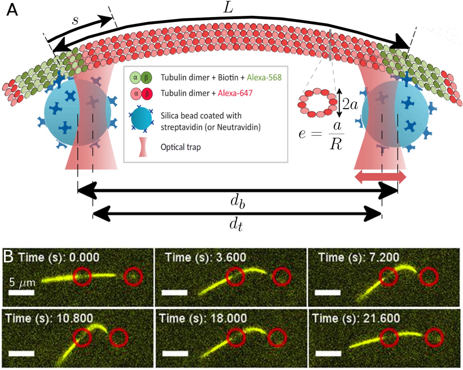
Probing the bending and stretching of microtubules using an optical trap.
(A) Schematic of the experimental setup for microtubule compression and stretching (note: not to-scale). Beads of radius 0.5 m manipulated through optical traps are attached to the filament via biotin-streptavidin bonds. The left trap remains fixed, while the right one is incrementally displaced towards or away. The bead separation is different from the trap separation due to the displacement between the centers of each bead and the corresponding trap. The force exerted by the traps on the beads is proportional to this displacement, with the constant of proportionality being the optical trap stiffness. The (effective) MT length is the length between the attachment points of the two beads (but note that multiple bonds may form). The arclength coordinate is measured from the left attachment point and takes value between 0 and : . A cross-sectional profile is shown to illustrate our definition of ‘eccentricity’ or ‘flatness’ (Equation 4) where is the length of the small axis and is the radius of the undeformed MT cross-section, taken to be nm in our simulations. (B) Series of fluorescence images from microtubule compression experiment. Trap positions represented through red circles of arbitrary size are drawn for illustration purposes and may not precisely represent actual trap positions, since neither beads nor traps are visible in fluorescence imaging. The mobile trap is moved progressively closer to the detection trap in the first four snapshots, resulting in increasingly larger MT buckling amplitudes. The mobile trap then reverses direction, decreasing the buckling amplitude as seen in the last two snapshots. The scale bar represents 5 m, the end-to-end length of the MT is approximately 18 m, and the length of the MT segment between the optical beads is 7.7 m.
Figure 2
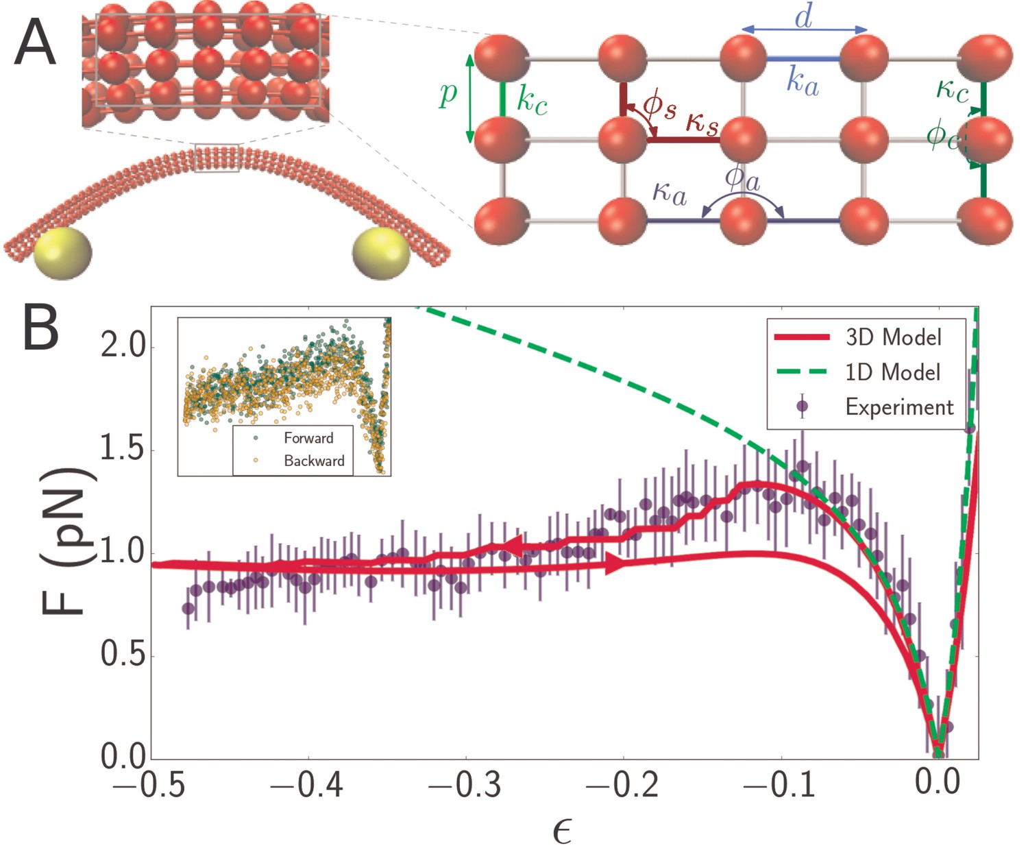
Discrete mechanical network model of microtubule.
(A) Schematic of spring network model of microtubule. Red particles discretize the filament while yellow particles represent the optical beads. Top inset: closeup of a region of the microtubule model, showing the 3D arrangement of the particles. Right inset: further closeup of the region, showing the defined interactions between particles. In the circumferential direction, ten particles are arranged in a circle of radius , (only three particles are shown in the inset) with neighboring pairs connected by springs of stiffness and rest length (light green). Neighboring triplets in the circumferential direction form an angle and are characterized by a bending energy interaction with parameter (dark green). In the axial direction, cross-sections are connected by springs of stiffness (light blue) running between pairs of corresponding particles. Bending in the axial direction is characterized by a parameter and the angle formed by neighboring triplets (dark blue). All other triplets of connected particles that do not run exclusively in the axial or circumferential direction encode a shearing interaction with energy given by (Table 1) with parameters and (yellow), where the stress-free shear angle is . (B) Force-strain curve for a microtubule of length 7.1 from experiment (blue) and simulation using a 1D model (green, dashed) or a 3D model (red). Arrows on the red curve indicate forward or backward directions in the compressive regime. The bending rigidity for the 1D model fit is . The fit parameters for the 3D model are GPa, MPa, and GPa. Errorbars are obtained by binning data spatially as well asaveraging over multiple runs. Inset: Raw data from individual ‘forward’ (green) and ‘backward’ (yellow) runs.
Figure 3
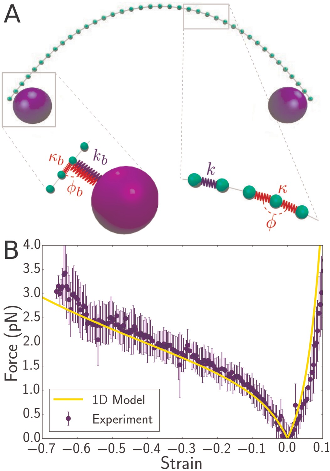
Discrete mechanical model of bacterial flagellum.
(A) Schematic of spring network model for bacterial flagellum. Green particles discretize the flagellum while blue particles represent the optical beads. Right inset: closeup of a region of the filament, showing that neighboring masses are connected by linear springs of stiffness which give rise to a stretching energy according to Equation 2, where is the stress-free length of the springs. In addition, each triplet of neighbors determines an angle which dictates the bending energy of the unit: (Equation 3). Left inset: closeup of the region where the bead connects to the flagellum. The bead particle is connected to a single particle of the flagellum by a very stiff spring of stress-free length corresponding to radius of the optical bead. In addition, there is a bending interaction , where is the angle determined by the bead, its connecting particle on the flagellum, and the latter’s left neighbor. (B) Force-strain curve from experiment (blue) and simulation (yellow) for a flagellum of length 4.1 . Errorbars are obtained by binning data spatially as well as averaging over multiple runs. The bending rigidity obtained from the fit is . The classical buckling force for a rod of the same length and bending rigidity with pinned boundary conditions is .
Figure 4
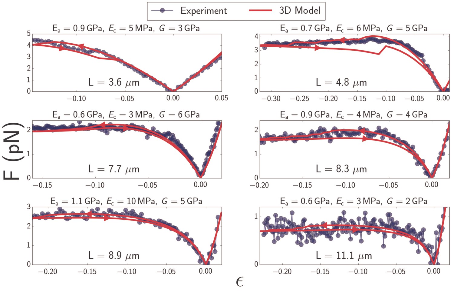
Plots of force as a function of strain (Equation 1) for microtubules ranging in length from to (blue).
Best-fit curves from simulation of the 3D model (red) and fit parameters (top) are shown for each plot. Arrows on the red curves indicate forward or backward directions in the compressive regime.
Figure 5
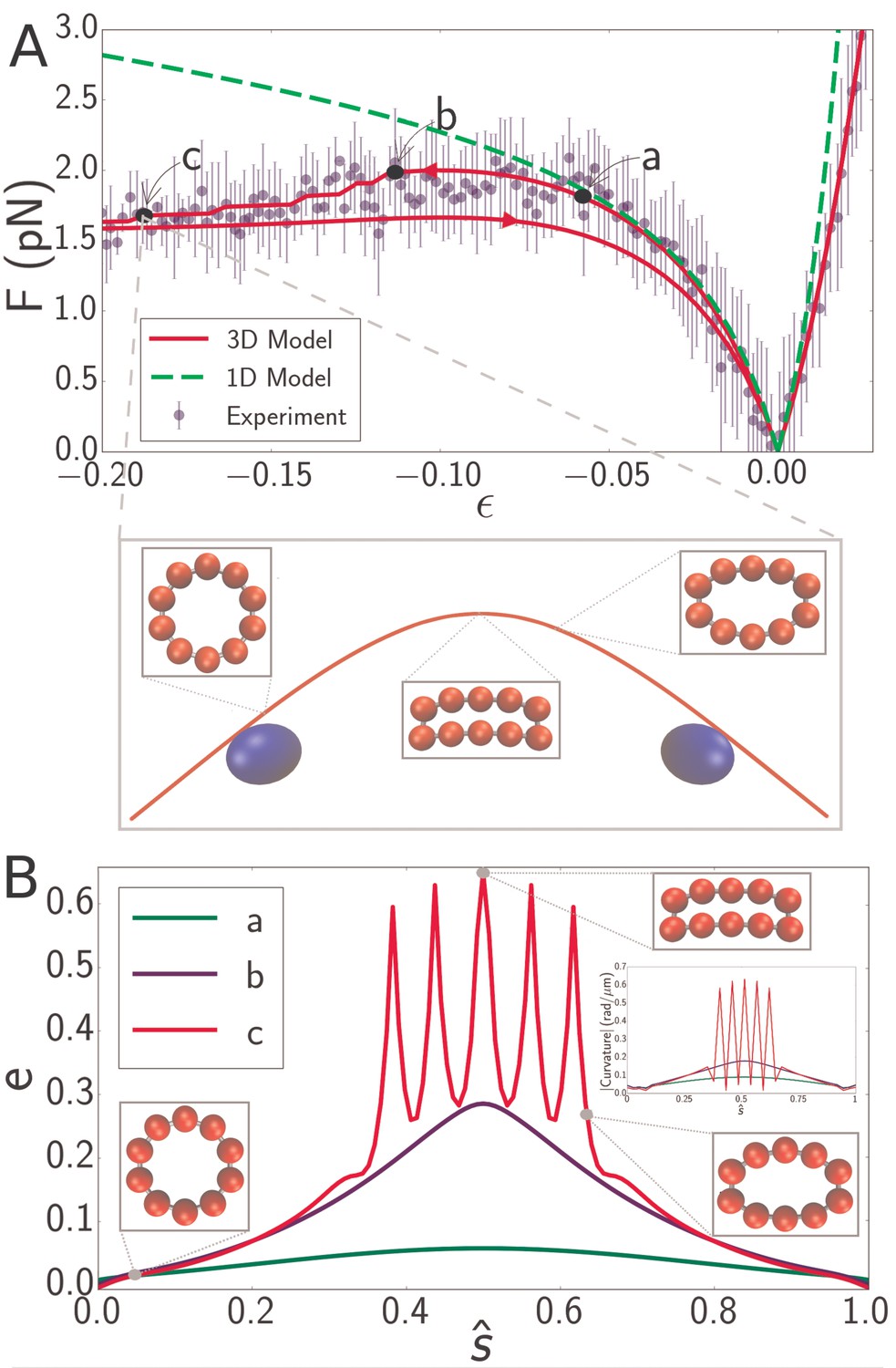
(A) Force-strain curve for a microtubule of length 8.3 from experiment (blue) and simulation using a 1D model (green, dashed) or a 3D model (red). Arrows on the red curve indicate forward or backward directions in the compressive regime. Errorbars are obtained by binning data spatially as well as averaging over multiple runs. The fit parameters for the 3D model are GPa, MPa, and GPa. The bending rigidity for the 1D model fit is . Labels a, b, and c indicate specific points in the 3D simulation model. (inset) Snapshot from simulation corresponding to the point labeled c. Smaller insets show the shape of the cross-section at indicated points. (B) Profiles of flatness (Equation 4) along the dimensionless arclength coordinate (see Figure 1A) at points identified in panel A as a (green), b (blue), and c (red). Three insets show the shape of the cross-section at indicated points for the curve labeled c (red). A fourth inset shows the curvature profiles corresponding, by color, to the flatness profiles in the main figure.
Figure 6
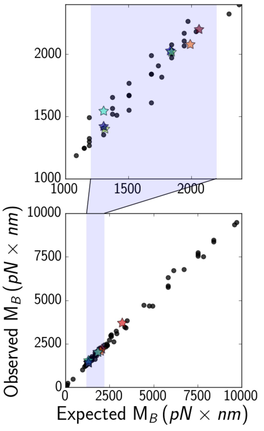
(bottom) Expected (Equation 6, with a numerical factor of unity) versus observed critical bending moments of simulated microtubules of various lengths, elastic moduli, and optical bead sizes.
Data points that correspond to actual experimental parameters are marked with stars, while the rest are marked with black circles. The shaded region is zoomed-in on (top), to show that most experimental points fall in the range about 1000–2000 .
Author response image 1
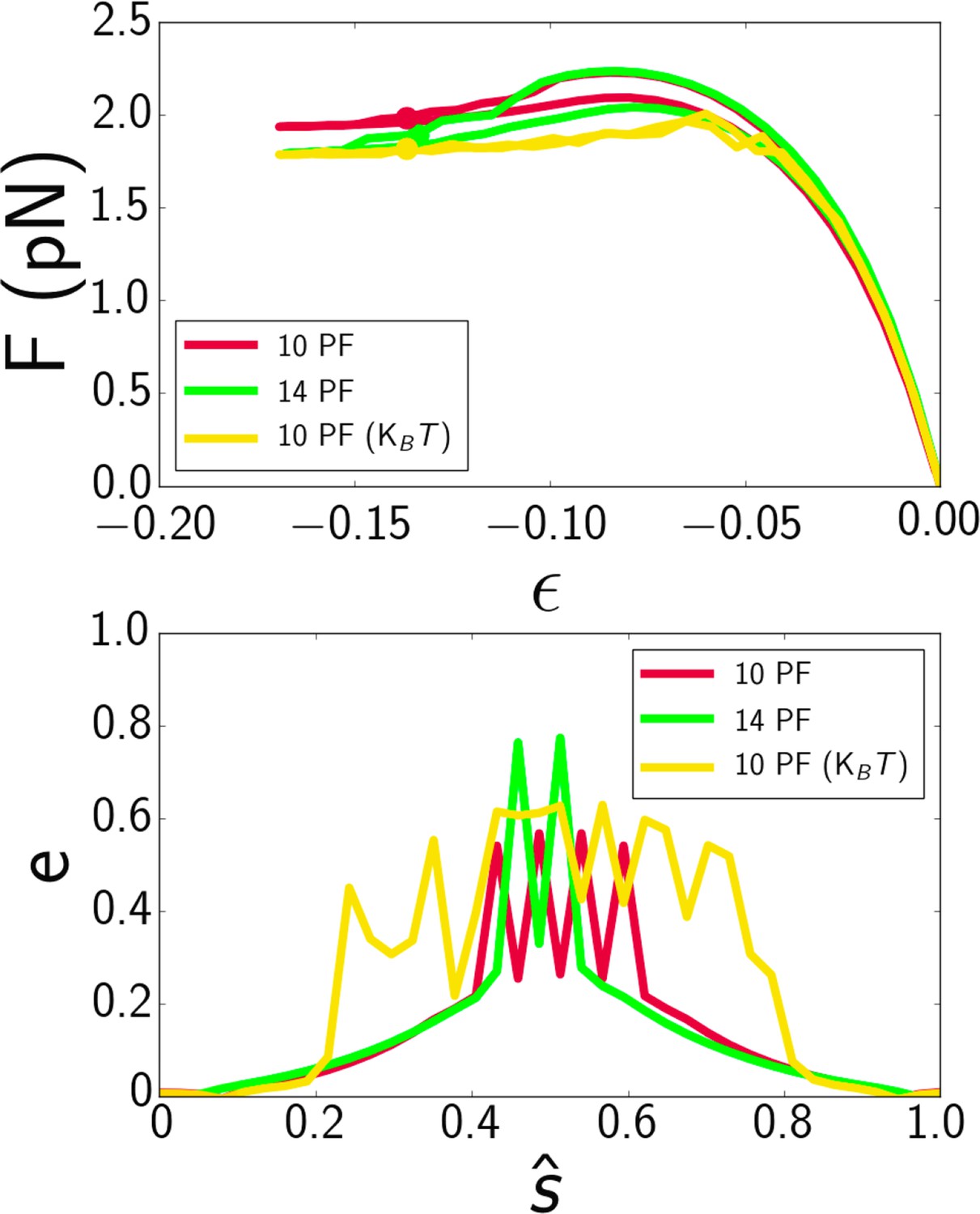
(A) Force-strain curve for a microtubule of length 7.7 μm from simulation using 10 protofilaments (red), 10 protofilaments with thermal noise (yellow), and 14 protofilaments (green).
The fit parameters are E a = 0.6 GPa, E c = 4 MPa, and G = 6 GPa. B) Profiles of flatness e (Eq. 4, manuscript) along the dimensionless arclength coordinate ŝ = s/L (see Fig. 1A, manuscript) at pointsidentified in panel A with dots.
Author response image 2
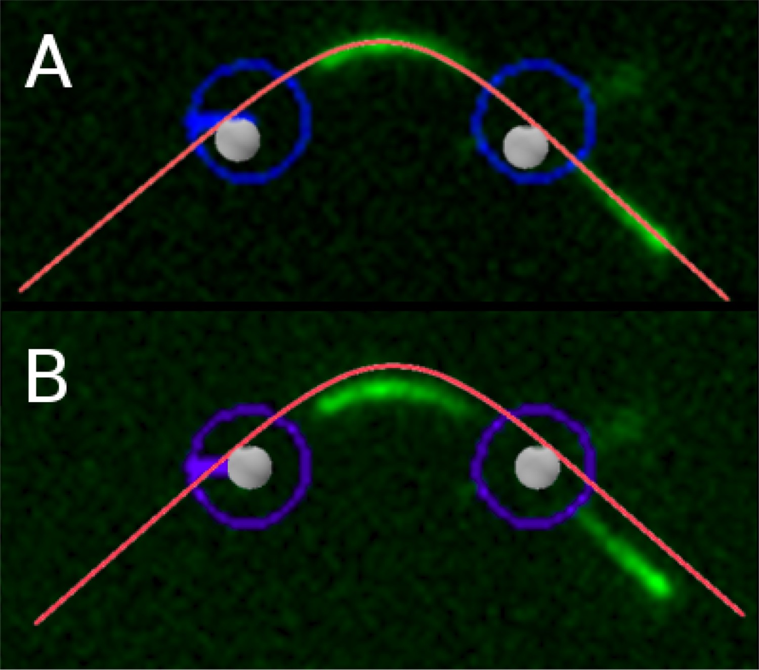
Comparison of shape between experiment (filament: (green); approx-imate trap positions: (blue)) and simulation (filament: (red); optical beads:(gray)) for a microtubule of length 8.3 μm (same as in figure 5, manuscript) at astrain ε ≈ −0.21 by A) aligning filament profiles and B) aligning bead positions(estimated).
https://doi.org/10.7554/eLife.34695.019Videos
Video 1
Microtubule buckling experiment, showing two ‘back-and-forth’ cycles.
The microtubule is labeled with fluorescent dye Alexa-647 and is actively kept in the focal plane. The scale bar represents 5 . Approximate positions of the optical traps are shown by red circles of arbitrary size.
Video 2
Flagellum buckling experiment.
(left) Simulation of microtubule buckling experiment shown in Figure 4, first panel. The length of the microtubule between the optical bead attachment points is 3.6 while the size of the optical beads is 0.5 . The shape of the cross-section located halfway along the microtubule is also shown. (right) Force-strain curves from experiment (blue) and simulation (red). The simulation curve is synchronized with the visualization on the left.
Video 3
Flagellum buckling experiment, showing three ‘back-and-forth’ cycles.
The scale bar represents 5 . Approximate positions of the optical traps are shown by green circles of arbitrary size. Measured force vector and magnitude are also indicated.
Tables
Table 1
List of microscopic parameters for the 3D model, their physical significance, the energy functional associated with them (Equation2 or Equation 3), and their connection to the relevant macroscopic elastic parameter.
Parameters, angles, and lengths are highlighted in Figure 2A. where nm and nm are the microtubule’s thickness and effective thickness (see Materials and methods), respectively and factors involving the Poisson ratios and are neglected.
| Microscopic | Physical | Associated | Relation to |
|---|---|---|---|
| Parameter | Significance | Energy | Macroscopic moduli |
| Axial stretching | |||
| Axial bending | |||
| Circumferential stretching | |||
| Circumferential bending | |||
| Shearing |
Table 2
Range of macroscopic elastic parameters that fit experimental data for microtubules and flagella.
https://doi.org/10.7554/eLife.34695.010| System | Fit parameters | Range that fits data |
|---|---|---|
| 0.6–1.1 GPa | ||
| Microtubule | 3–10 MPa | |
| 1.5–6 GPa | ||
| Flagellum | 3–5 |
Additional files
-
Source Code 1
Source code files and source data for Figure 6 and source code files along with instructions for generating the data in Figure 2.
- https://doi.org/10.7554/eLife.34695.013
-
Supplementary file 1
List of parameters used in the paper.
- https://doi.org/10.7554/eLife.34695.014
-
Supplementary file 2
(left) Summary of previous experiments examining microtubule stiffness, adapted from (Hawkins et al., 2010).
(right) Box plot comparing bending stiffness values obtained via thermal fluctuations and mechanicalbending for microtubules stabilized with GDP Tubulin + Taxol (orange), GMPCPP Tubulin (green), and GDP Tubulin (blue)
- https://doi.org/10.7554/eLife.34695.015
-
Transparent reporting form
- https://doi.org/10.7554/eLife.34695.016
Download links
A two-part list of links to download the article, or parts of the article, in various formats.
Downloads (link to download the article as PDF)
Open citations (links to open the citations from this article in various online reference manager services)
Cite this article (links to download the citations from this article in formats compatible with various reference manager tools)
Microtubules soften due to cross-sectional flattening
eLife 7:e34695.
https://doi.org/10.7554/eLife.34695


