Figures and data in Chronology of motor-mediated microtubule streaming

Figures
Videos
Tables
Additional files

10 figures, 4 videos, 3 tables and 2 additional files

Figures

Figure 1

Download asset Open asset

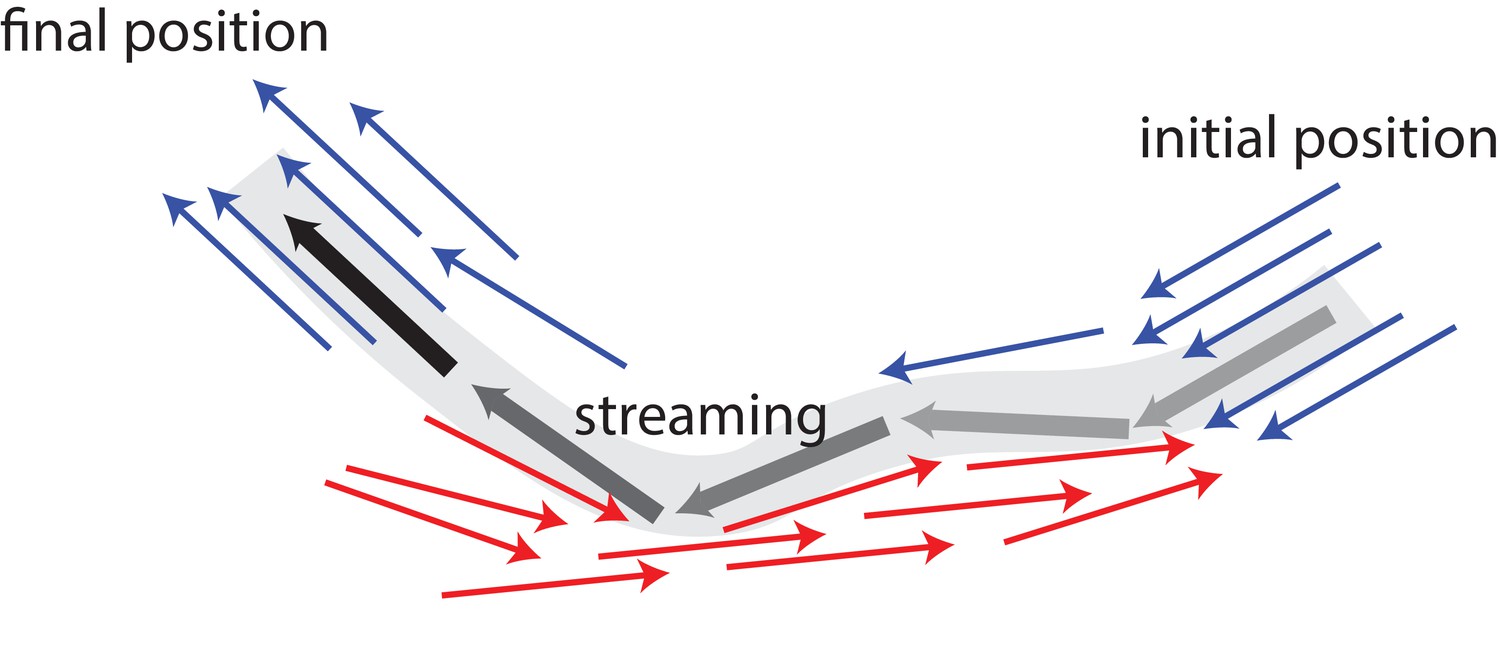
Schematic illustrating MT bundling and streaming.

Polar-aligned MTs are coloured blue, and antialigned MTs are coloured red. The grey/black MT is transported from its initial position (grey), in one polar-aligned bundle, to its final position (black), to another polar-aligned bundle, via a stream.

https://doi.org/10.7554/eLife.39694.002

Figure 2

Download asset Open asset

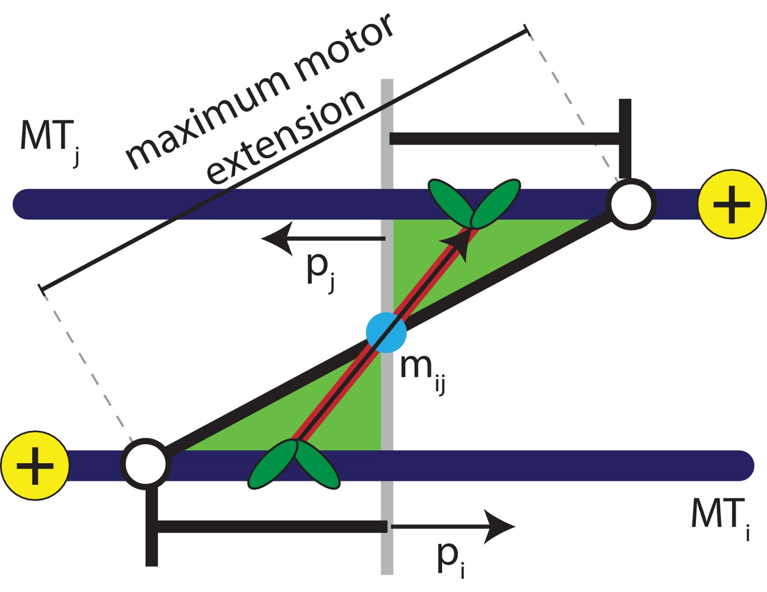
Schematic explaining the conditions that satisfy the antialigned motor potential.

The vectors, $𝐩_{i}$ , $𝐩_{j}$ , and $𝐦_{i j}$ , represent the unit orientation vectors of MT $i$ , MT $j$ , and the motor vector that crosslinks the beads of adjacent MTs, respectively. The white circles represent the maximum extension of motors between the two MTs.

https://doi.org/10.7554/eLife.39694.003

Figure 3 with 10 supplements

Download asset Open asset

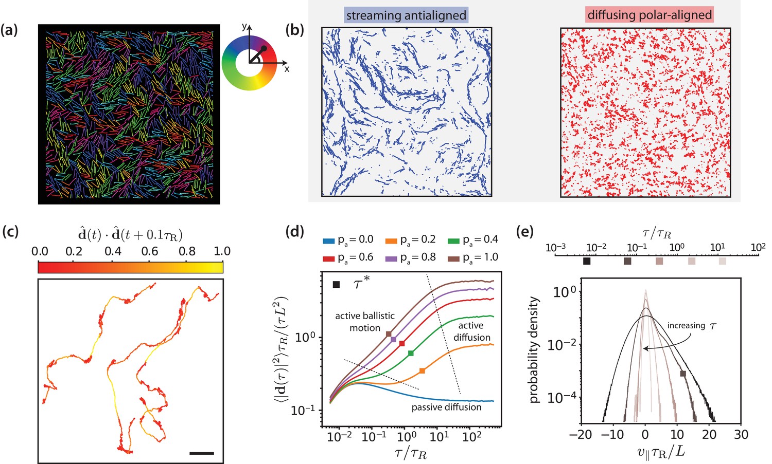
Motor-driven and diffusive motion of MTs.

(a) Simulation snapshot of MTs organised by effective motors. MTs are coloured based on their orientation according to the colour legend on the right. See corresponding Video 1. (b) Trajectories of MTs within a time window of 1.2 $τ_{R}$ separated based on the antialigned and polar-aligned categories. See corresponding Video 2. (c) Plots of the trajectory of three selected MTs coloured based on the correlation of adjacent steps in their velocity. The entire trajectory is for a time window of $300 τ_{R}$ is the unit vector of MT displacement. The fast-streaming and slow-diffusion modes correspond with the yellow and red parts of the trajectories respectively. The scale bar corresponds to the length of five MTs. See corresponding Video 3. (d) MSD/lag time for various levels of activity $p_{a}$ and MT density $ϕ = 0.3$ . The time scale of maximal activity, $τ^{*}$ , calculated from the time of maximal $v_{∥}$ skew is indicated by the squares on the curves. (e) Histogram of parallel velocity for various $τ$ . The curve closest corresponding to the time scale of maximal activity, $τ^{*}$ , is indicated with a box marker. All figures are for $ϕ = 0.3$ . (a), (b), (c) and (e) are for $p_{a} = 1.0$ .

https://doi.org/10.7554/eLife.39694.004

Figure 3—source data 1 Source data for graphs shown in Figure 3 (d,e).: https://doi.org/10.7554/eLife.39694.015
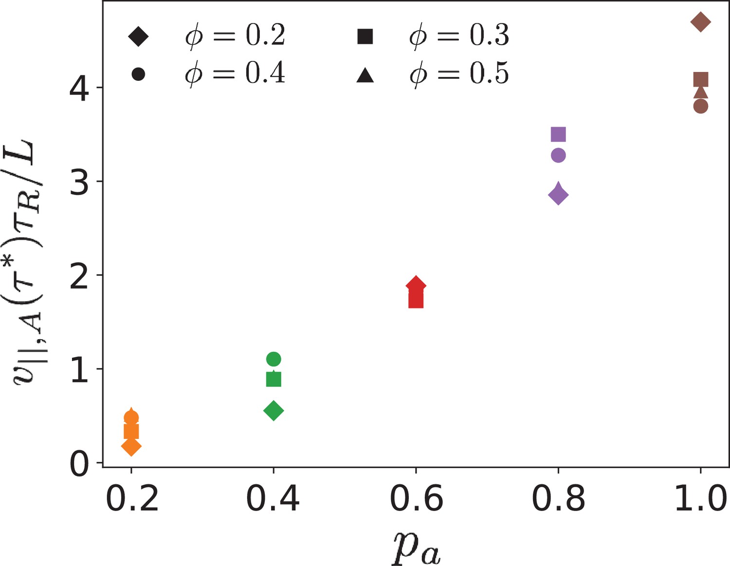
Download elife-39694-fig3-data1-v2.zip

Figure 3—figure supplement 1

Download asset Open asset

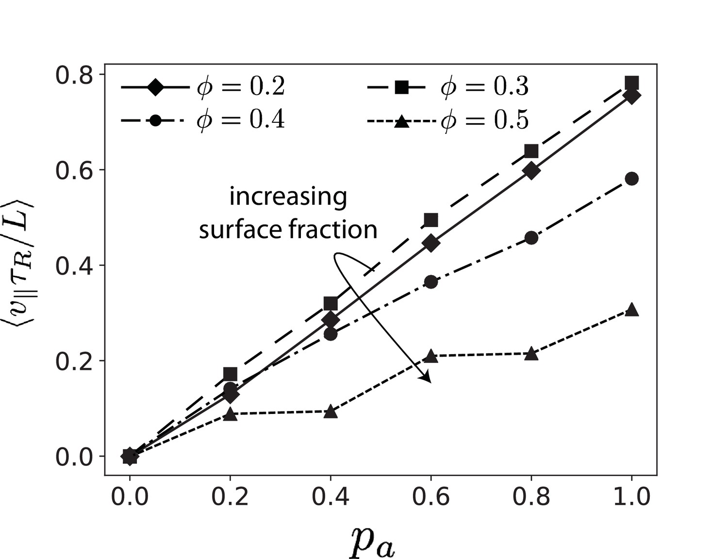
Parallel velocity $v_{∥}$ , extrapolated to $τ = 0$ as function of the antialigned motor probability $p_{a}$ for various MT surface fractions $ϕ$ .
https://doi.org/10.7554/eLife.39694.005

Figure 3—figure supplement 2

Download asset Open asset

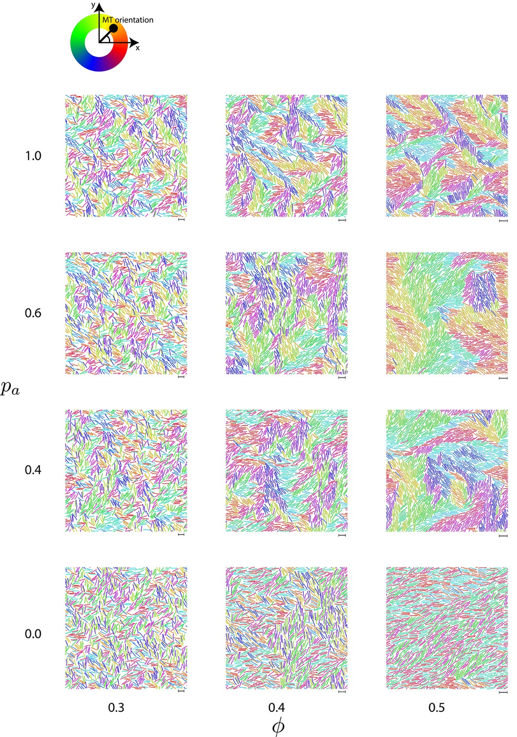
Simulation snapshots at steady state for various antialigned motor probabilities $p_{a}$ and MT surface fractions $ϕ$ .

Data for $0.0 < p_{a} \leq 1.0$ and $0.3 < ϕ < 0.5$ .

The surface fractions of MTs are varied by changing the size of the periodic box, while keeping the number of MTs constant. The scale bars correspond to the length of a single MT. The colours represent the orientation of the polar MTs with respect to the system reference frame according to the colour wheel above.

https://doi.org/10.7554/eLife.39694.006

Figure 3—figure supplement 3

Download asset Open asset

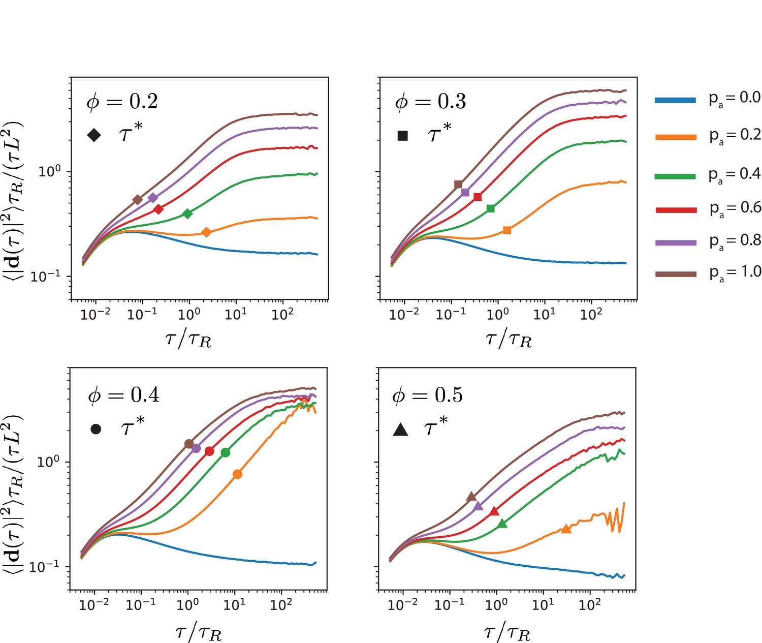
Translational MT mean squared displacements for various antialigned motor probilities $p_{a}$ and MT surface fractions $ϕ$ .

The symbols on the plots indicate the time scale at which the parallel velocity is maximally skewed due to active forces.

https://doi.org/10.7554/eLife.39694.007

Figure 3—figure supplement 4

Download asset Open asset

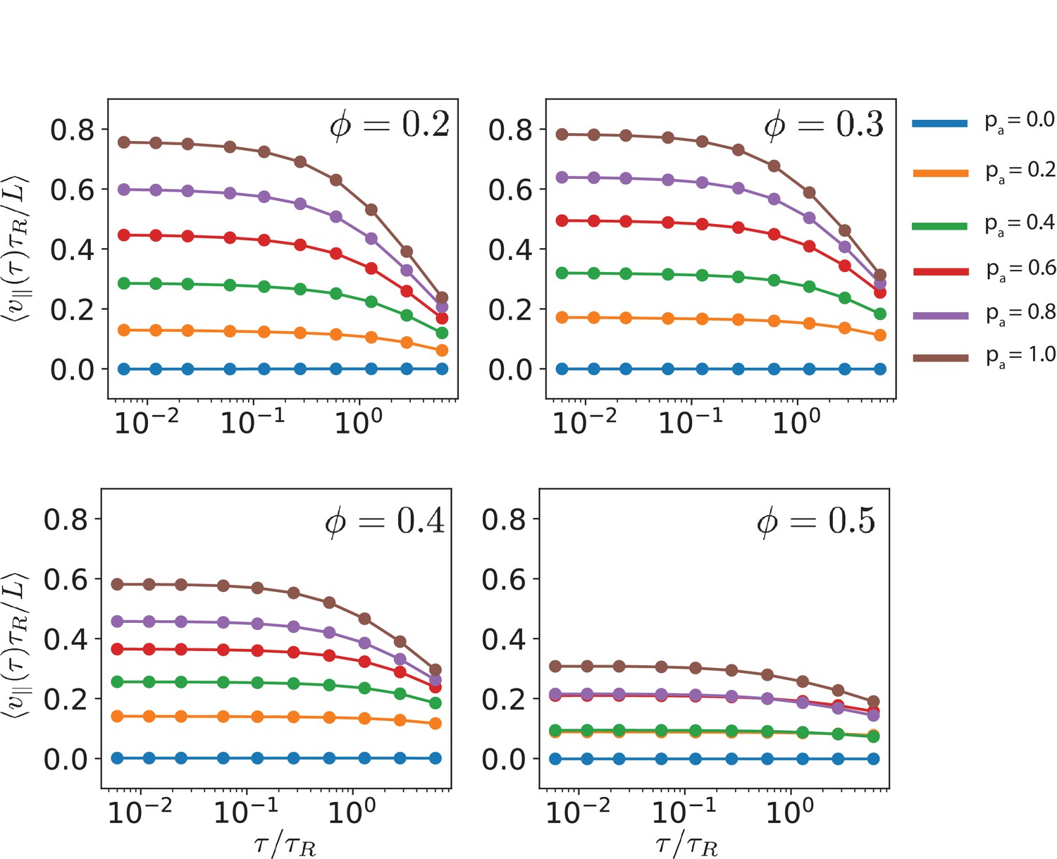
Parallel velocity $v_{∥}$ as a function of the time window $τ$ for various antialigned motor probabilities $p_{a}$ and MT surface fractions $ϕ$ .
https://doi.org/10.7554/eLife.39694.008

Figure 3—figure supplement 5

Download asset Open asset

Maximum parallel MT velocities $v_{∥, A} (τ^{*})$ as function of the antialigned motor probability $p_{a}$ for various MT surface fractions $ϕ$ .
https://doi.org/10.7554/eLife.39694.009

Figure 3—figure supplement 6

Download asset Open asset

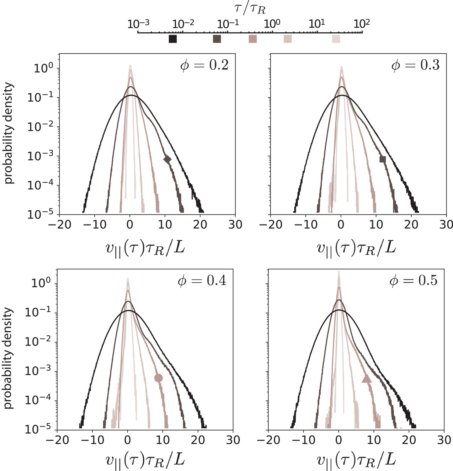
Histogram of $v_{∥}$ for various MT surface fractions $ϕ$ and five time windows $τ$ .

The darkness of the curve represents the time window used to measure the parallel velocity. The darkest-coloured curve represents the parallel velocity obtained for the shortest time window, and the lightest-coloured curve is obtained from the longest time window. The box symbols mark the displacement distributions that are closest to the distribution which is most skewed.

https://doi.org/10.7554/eLife.39694.010

Figure 3—figure supplement 7

Download asset Open asset

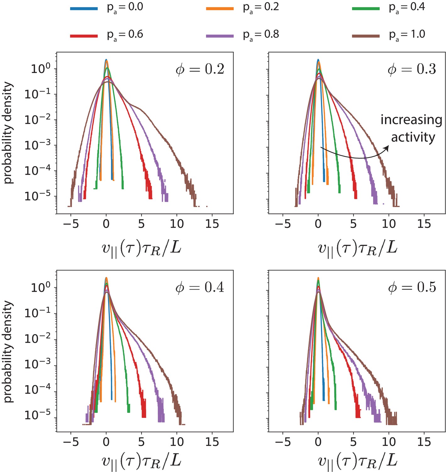
Histogram of $v_{∥} (τ^{*})$ for various $p_{a}$ and $ϕ$ .

The duration of the time window corresponds to the maximal skew, see Figure 6. This indicates the structure of the velocity distribution when the skew is maximal. The ordinate axis is log scaled to show the deviation of the distribution from a Gaussian, which would appear as a symmetric inverted parabola.

https://doi.org/10.7554/eLife.39694.011

Figure 3—figure supplement 8

Download asset Open asset

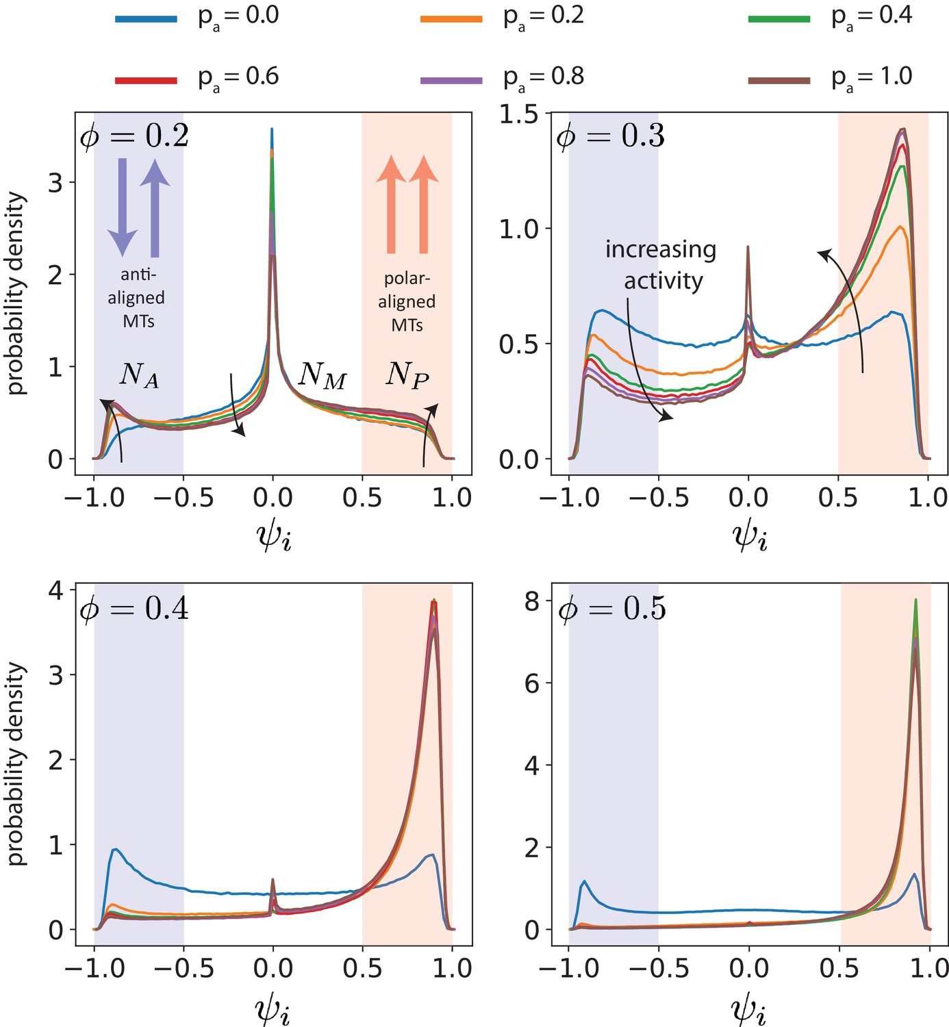
Probability densities of the MT local polar order parameter $ψ_{i}$ .

Data for various antialigned motor probabilities $p_{a}$ and MT surface fractions $ϕ$ . The arrows indicate the changes of the probability densities for increasing activity. A, M and P indicate $ψ_{i} \leq - 0.5$ (green), $- 0.5 < ψ_{i} < 0.5$ (white), $ψ_{i} \geq 0.5$ (blue), respectively. $N_{A}$ , $N_{m}$ and $N_{P}$ are the number of MTs in antialigned, perpendicular and polar-aligned environments respectively. Note that the scale of the ordinate is different for each MT surface fraction.

https://doi.org/10.7554/eLife.39694.012

Figure 3—figure supplement 9

Download asset Open asset

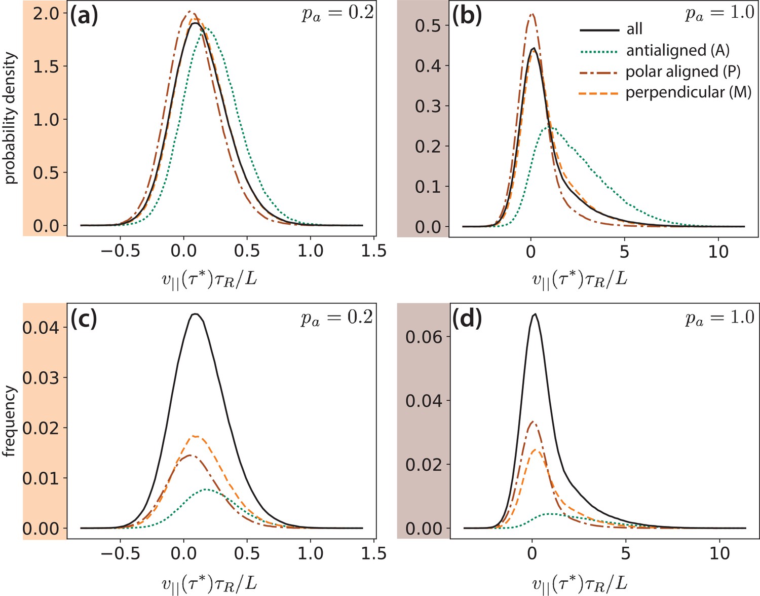
MT parallel velocity distributions.

Data for $v_{∥}$ for a time window of duration $τ^{*}$ and $ϕ = 0.3$ , decomposed based on MT environments (**A, M, P**) determined by their local polar order parameter, $ψ_{i}$ , see Figure 8. (a) and (b) show probability density histograms of $v_{∥} (τ^{*})$ for $p_{a} = 0.2$ and $1.0$ , respectively. (c) and (d) show frequencies of occurrence of $v_{∥} (τ^{*})$ for $p_{a} = 0.2$ and $1.0$ , respectively. The sum of the decomposed curves in (c) and (d) gives the solid curves.

https://doi.org/10.7554/eLife.39694.013

Figure 3—figure supplement 10

Download asset Open asset

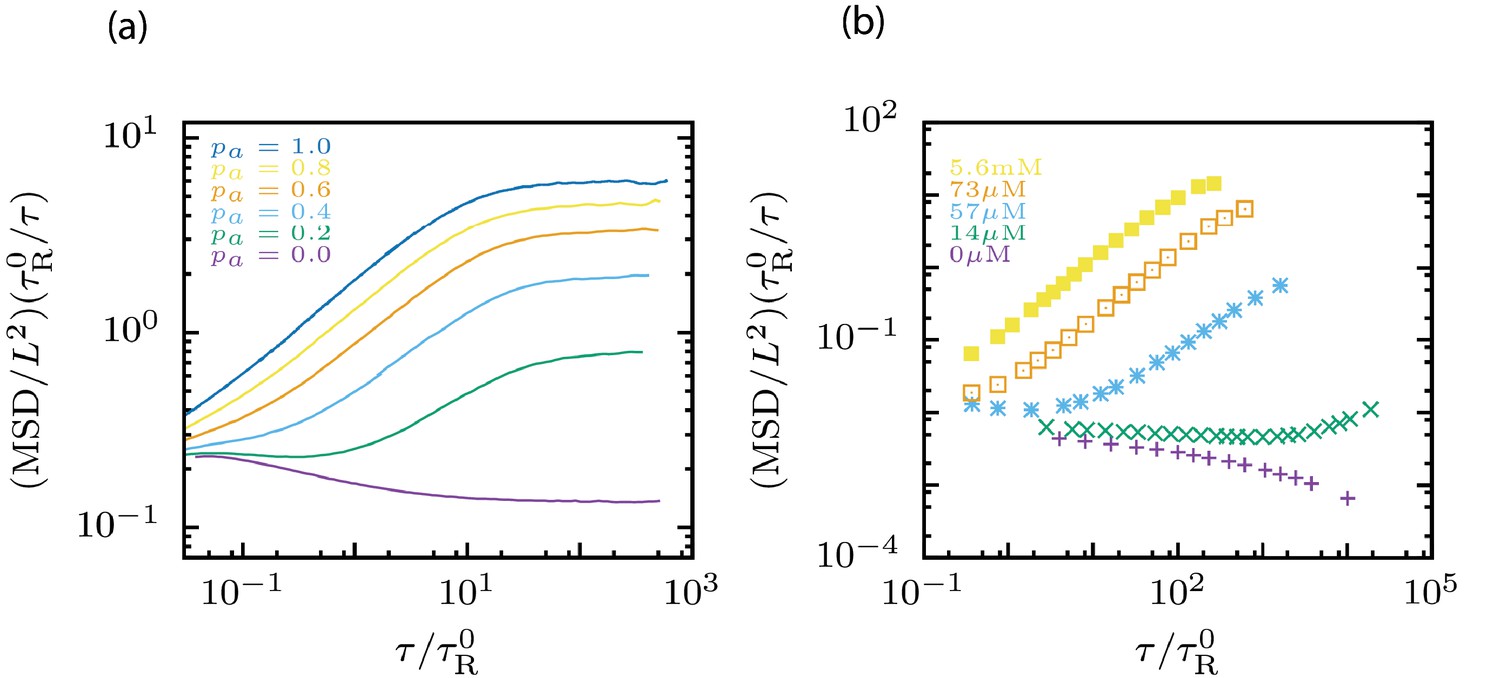
MT mean squared displacements: computer simulation and experimental data.

(a) Normalized MSD curves from our simulations for several motor probabilities $p_{a}$ . (b) Normalized MSD curves as a function of lag time for experiments eLifeMediumGrey (Sanchez et al., 2012) *for selected ATP concentrations. Here $L$ is the filament length, $τ_{R}^{0}$ the single filament rotation time and $τ$ the lag time.*

https://doi.org/10.7554/eLife.39694.014

Figure 4 with 1 supplement

Download asset Open asset

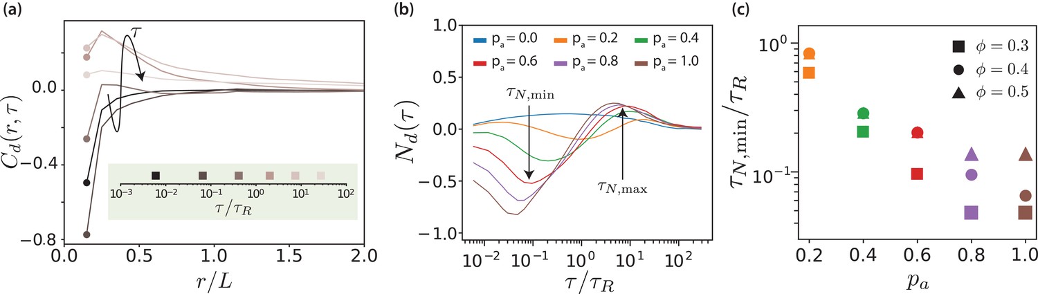
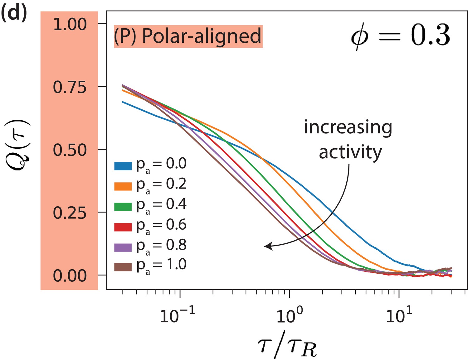
Displacement correlations of MTs.

(a) Spatio-temporal correlation function $C_{d} (r, τ)$ for $ϕ = 0.3$ and $p_{a} = 1.0$ , for some selected lag times. The arrow and the colours of the curves indicate increasing lag time. The lag times are picked from a logarithmic scale. (b) Neighbour correlation function $N_{d} (τ) = C_{d} (σ, τ)$ for $ϕ = 0.3$ and various $p_{a}$ values. (c) The sliding time scale indicated by $τ_{N, \min}$ is shown for various MT surface fractions and $p_{a}$ values.

https://doi.org/10.7554/eLife.39694.020

Figure 4—source data 1 Source data for graphs shown in Figure 4 (a,b,c).: https://doi.org/10.7554/eLife.39694.022
Download elife-39694-fig4-data1-v2.zip

Figure 4—figure supplement 1

Download asset Open asset

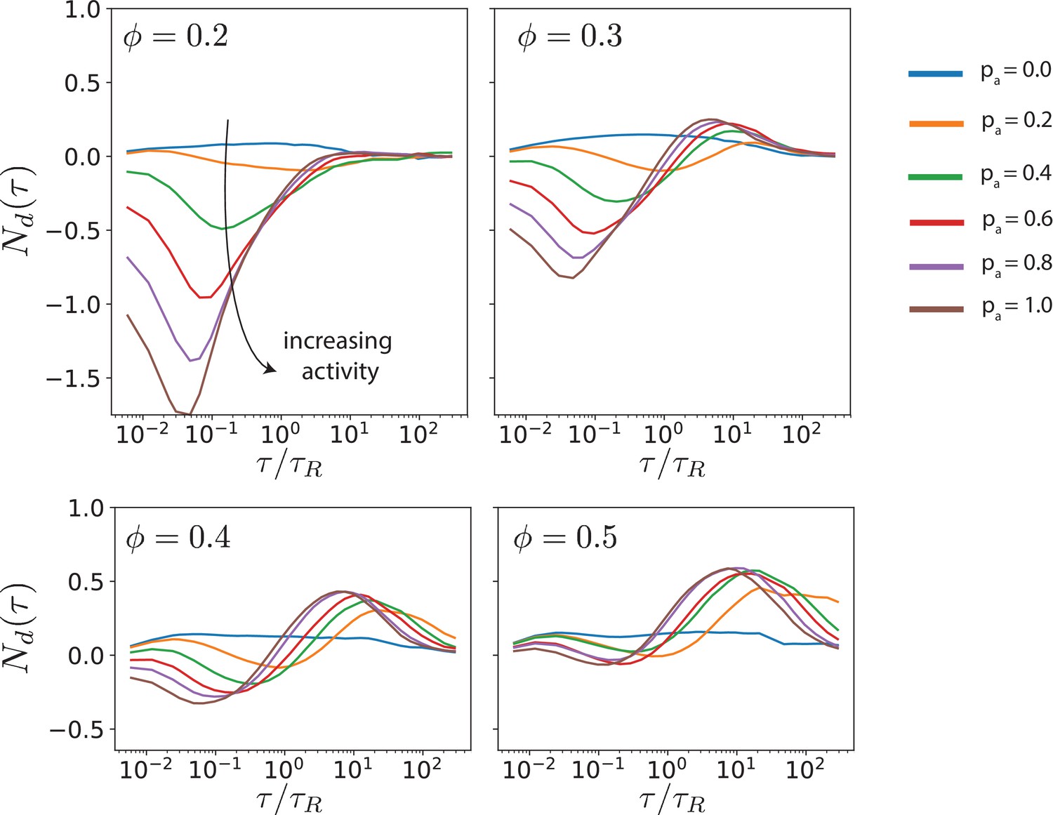
Neighbour displacement correlation function $N_{d} (τ)$ for various MT surface fractions $ϕ$ and antialigned motor probabilities $p_{a}$ .

The lag times at which the minimum and maximum of $N_{d} (τ)$ occur are $τ_{N, min}$ and $τ_{N, max}$ , respectively.

https://doi.org/10.7554/eLife.39694.021

Figure 5 with 3 supplements

Download asset Open asset

Local polar order of MTs.

(a) Mean local polar order $⟨ ψ_{i} (τ) ⟩$ for $p_{a} = 0.0$ and $p_{a} = 1.0$ at $ϕ = 0.3$ , for MTs starting from antialigned (dotted line) and aligned (solid line) environments at $τ = 0$ . (b) Deviation of local polar order $Q (τ)$ for $ϕ = 0.3$ for various $p_{a}$ for antialigned MTs. (c) Relaxation time for the polar order parameter, $τ_{Q / 2}$ for various $p_{a}$ and $ϕ$ , estimated by the time for $Q$ to decrease to half its initial value.

https://doi.org/10.7554/eLife.39694.023

Figure 5—source data 1 Source data for graphs shown in Figure 5 (a,b,c).: https://doi.org/10.7554/eLife.39694.027
Download elife-39694-fig5-data1-v2.zip

Figure 5—figure supplement 1

Download asset Open asset

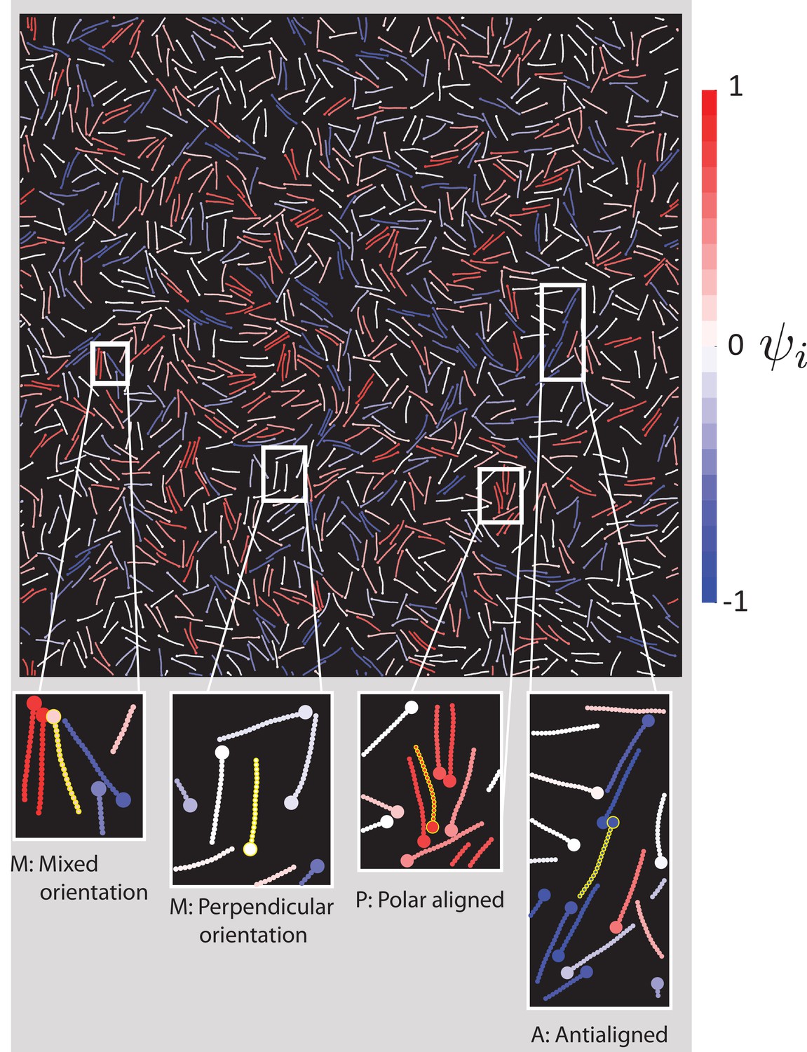
MTs coloured based on their local polar order parameter $ψ_{i}$ for $p_{a} = 1.0$ , $ϕ = 1.0$ .

The colour corresponding to $- 1 < ψ_{i} < 1$ is given on the right. Zoomed in illustrations of MTs show examples of MTs in the three $ψ_{i}$ categories distinguished in Figure 8. The MT in question is highlighted in yellow in the zoomed in graphics. (M) $ψ_{i} \approx 0$ values can occur either when MTs are perpendicularly oriented with respect to its surrounding or when MTs have neighbours which are both polar-aligned and antialigned. (P) $ψ_{i} > 0.5$ occurs when MTs have neighbours which are mostly polar-aligned. (A) $ψ_{i} < - 0.5$ occurs when MTs have neighbours which are mostly antialigned.

https://doi.org/10.7554/eLife.39694.024

Figure 5—figure supplement 2

Download asset Open asset

Deviation from local polar order $Q (τ)$ as function of the lag time $τ$ for various antialigned motor probabilities $p_{a}$ for polar-aligned MTs.
https://doi.org/10.7554/eLife.39694.025

Figure 5—figure supplement 3

Download asset Open asset

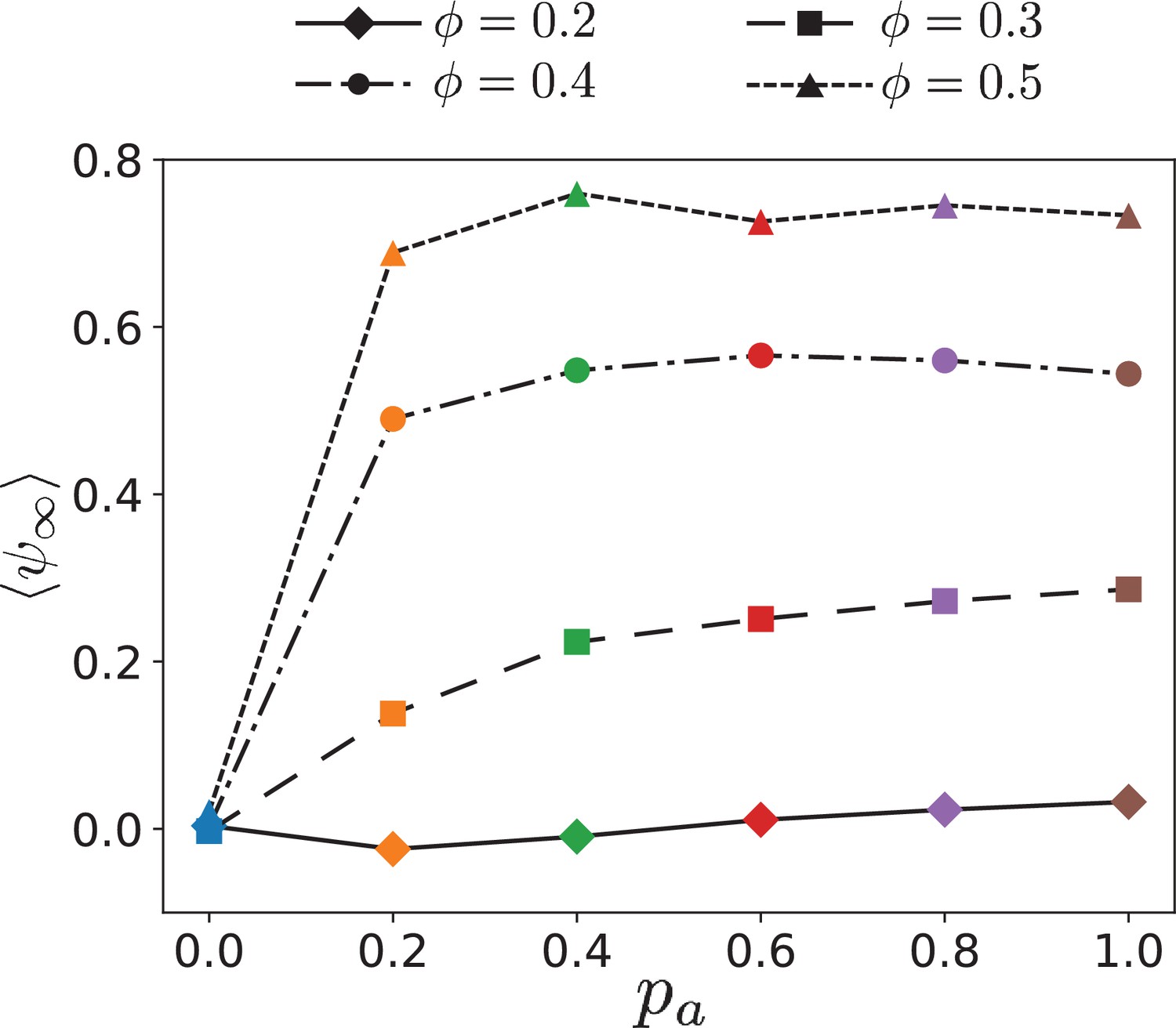
Mean local polar order parameter of MTs at long times, $⟨ ψ_{\infty} ⟩$ , for various surface fractions $ϕ$ and antialigned motor probabilities $p_{a}$ .
https://doi.org/10.7554/eLife.39694.026

Figure 6 with 3 supplements

Download asset Open asset

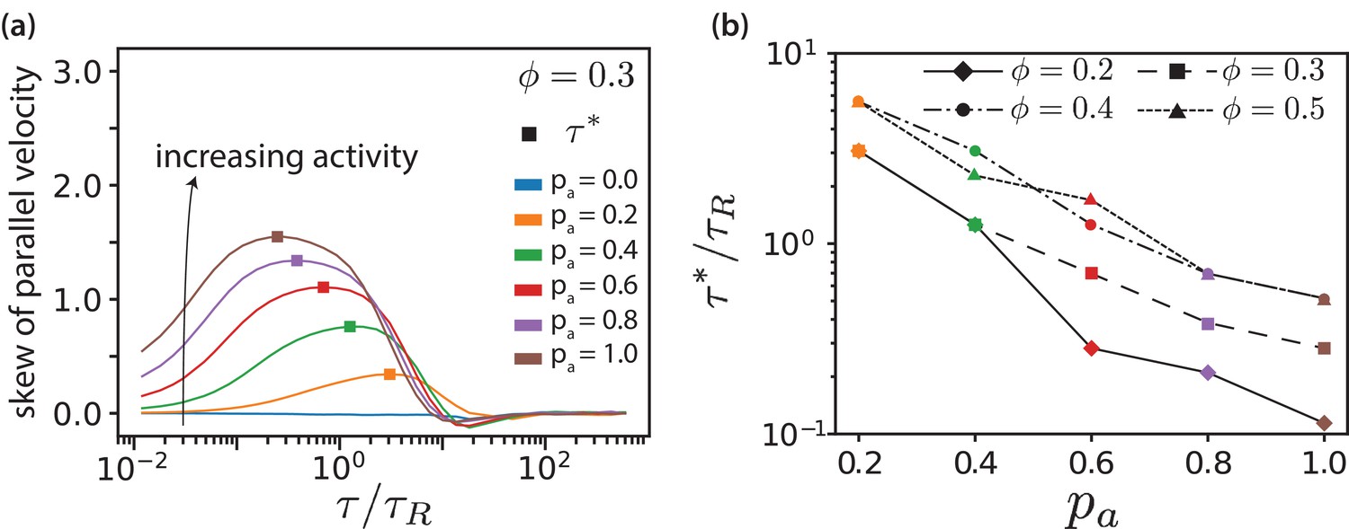
MT parallel velocity distributions.

(a) Skew of parallel velocity ( $v_{∥}$ ) distribution computed as function of lag times for different $p_{a}$ for $ϕ = 0.3$ . The probability distributions that correspond to the maximal skew are shown in Figure 3—figure supplement 6 together with distributions for few other lag times. (b) Lag time at which maximal skew is observed in the $v_{∥} (τ)$ distribution (compare Figure 1). The ordinate is log-scaled to show that $τ^{*}$ is exponentially decreasing with $p_{a}$ .

https://doi.org/10.7554/eLife.39694.028

Figure 6—source data 1 Source data for graphs shown in Figure 6 (a,b).: https://doi.org/10.7554/eLife.39694.032
Download elife-39694-fig6-data1-v2.zip

Figure 6—figure supplement 1

Download asset Open asset

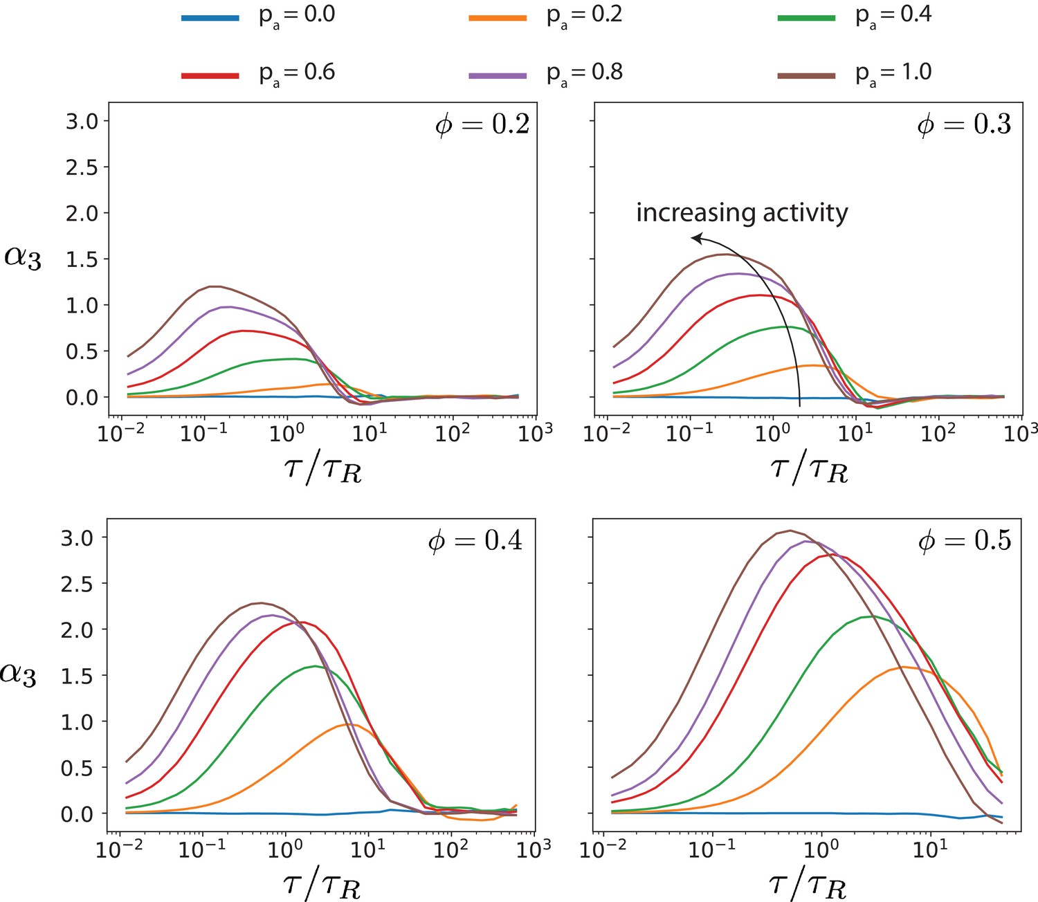
Skews $α_{3}$ of parallel velocity distributions ( $v_{∥}$ ) (Fig.

Figure 6) computed as a function of lag times for various antialigned motor probabilities $p_{a}$ and surface fractions $ϕ$ . The probability distributions that correspond to the maximal skew are shown in Figure 6 together with distributions for few other lag times. The ordinate scale is the same for comparison of the skews for different MT surface fractions.

https://doi.org/10.7554/eLife.39694.029

Figure 6—figure supplement 2

Download asset Open asset

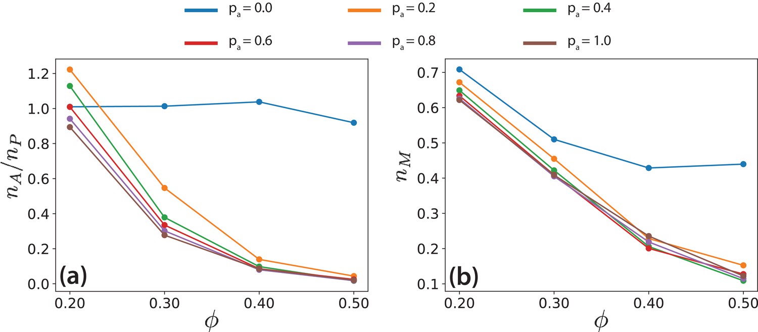
Ratios of MT populations in environments with different local polar order.

Ratios of MT populations in (a) antialigned to polar-aligned environments, and (b) perpendicular environments to total number of MTs, for various MT surface fractions $ϕ$ and antialigned motor probabilities $p_{a}$ .

https://doi.org/10.7554/eLife.39694.030

Figure 6—figure supplement 3

Download asset Open asset

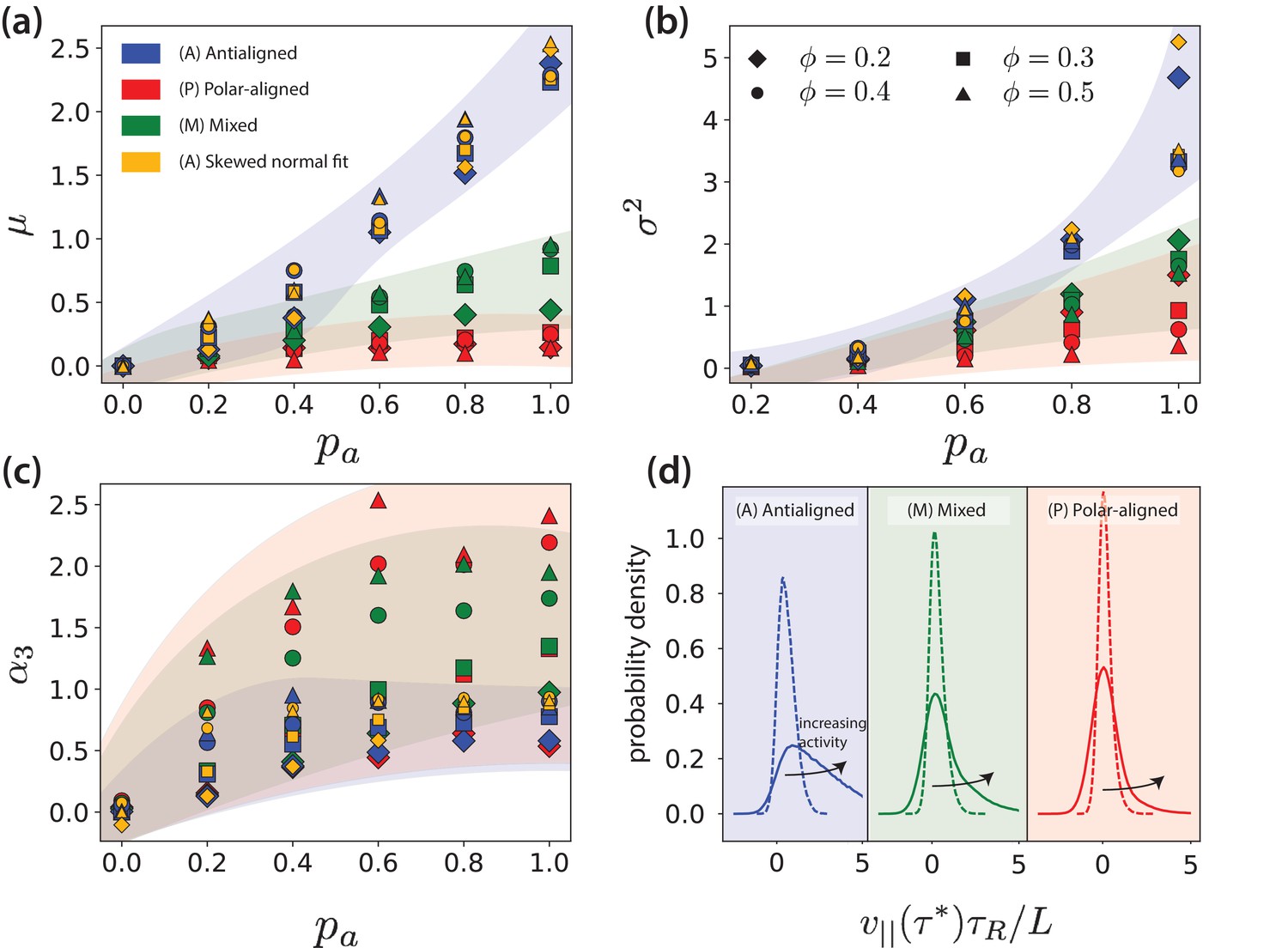
First three moments of the parallel velocity ( $v_{∥}$ ) distribution.

First three moments, (a) mean, (b) variance, (c) skew of the $v_{∥}$ distribution for a time window of duration $τ^{*}$ for MTs in (A) antialigned, ( $ψ_{i} < - 0.5$ , blue), (P) polar-aligned ( $ψ_{i} > 0.5$ , red), and (M) mixed ( $| ψ_{i} | \leq 0.5$ , green) environments, for different $ϕ$ and $p_{a}$ . The blue, red and green markers indicate moment calculated from raw data. The yellow markers are obtained from calculating moments from fits to the antialigned parallel MT velocity distribution $v_{∥, A}$ . (d) Example of differences in structures of $v_{∥}$ distributions due to increasing activity from $p_{a} = 0.4$ (dotted line) to $p_{a} = 1.0$ (solid line) for $ϕ = 0.3$ , for A, P and M categories of MT environment.

https://doi.org/10.7554/eLife.39694.031

Figure 7 with 1 supplement

Download asset Open asset

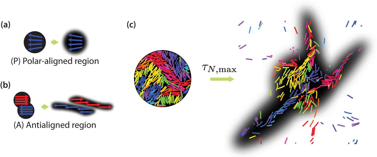
Collective motion of MTs.

Schematic of expected evolution of photobleached regions in (a) polar-aligned and (b) antialigned regions. (c) Selectively visualised MTs in a circular region within the simulation box, and their evolution after a time of $τ_{N, \max}$ , for $ϕ = 0.4$ and $p_{a} = 1.0$ . The black backgrounds are predictions of FRAP results.

https://doi.org/10.7554/eLife.39694.033

Figure 7—figure supplement 1

Download asset Open asset

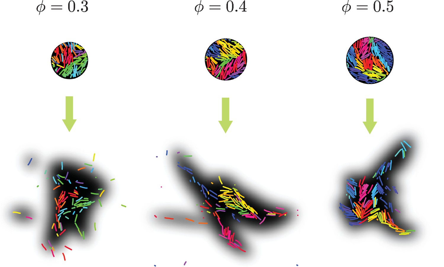
FRAP-like predictions for various MT surface fractions $ϕ$ .

Predictions for photobleaching experiments with $ϕ = 0.3$ , $0.4$ , and $0.5$ . MTs retain the orientation colour from when they were tagged at $t = 0$ . The black shadow shows our predictions for photobleaching experiments at time $τ_{N, \max}$ after bleaching a circular patch.

https://doi.org/10.7554/eLife.39694.034

Figure 8

Download asset Open asset

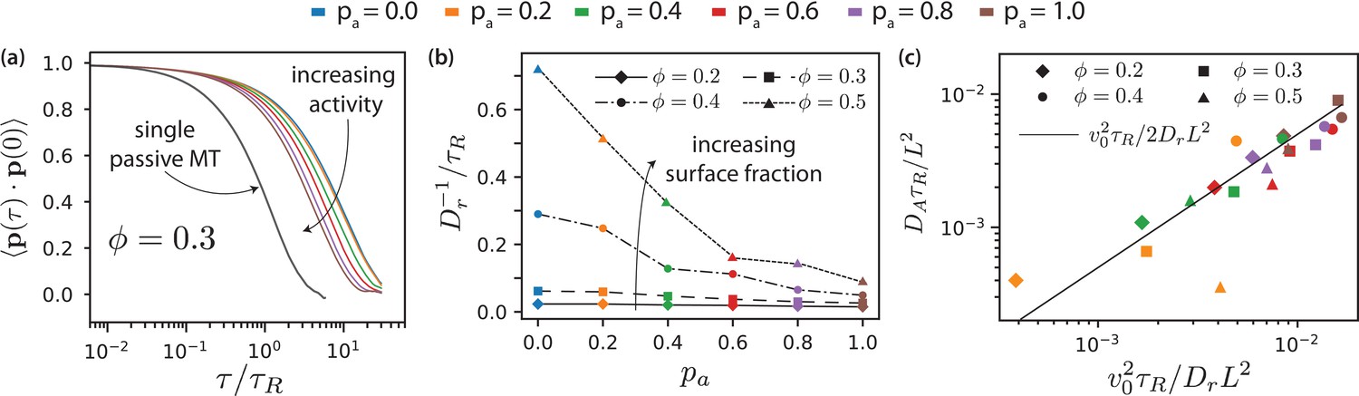
MT orientational correlation and active diffusion.

(a) Orientational correlation function for $ϕ = 0.3$ for various antialigned motor probabilities $p_{a}$ . (b) Inverse of rotational diffusion, $τ_{r}$ for various antialigned motor probabilities $p_{a}$ and surface fractions $ϕ$ (c) Active diffusion coefficient $D_{A}$ for $p_{a} = 1$ .

https://doi.org/10.7554/eLife.39694.035

Figure 8—source data 1 Source data for graphs shown in Figure 8 (a,a-one filament,b,c).: https://doi.org/10.7554/eLife.39694.036
Download elife-39694-fig8-data1-v2.zip

Figure 9

Download asset Open asset

Chronology of MT streaming. Events from antialigned MT propulsion to MT rotation (left to right) which make up the streaming process, for various antialigned motor probabilities $p_{a}$ and surface fractions $ϕ = 0.3$ , $ϕ = 0.4$ , and (c) $ϕ = 0.5$ as indicated.
https://doi.org/10.7554/eLife.39694.037

Figure 9—source data 1 Source data for graphs shown in Figure 9 (a,b,c).: https://doi.org/10.7554/eLife.39694.038
Download elife-39694-fig9-data1-v2.zip

Author response image 1

Download asset Open asset

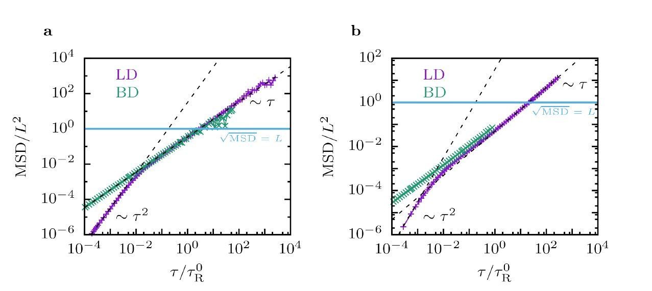
Mean squared displacements of filaments obtained from Langevin Dynamics (LD) and Brownian Dynamics (BD), for single filaments (left) and filaments in suspensions with packing fraction 𝜙 = 0.3 (right).

The simulation parameters are the same as in the manuscript.

https://doi.org/10.7554/eLife.39694.045

Videos

Video 1

Download asset

posterframe for video — Steady-state dynamics of the MT-effective motor system shown in Figure 3(a) for 100 $τ_{R}$ .

MTs are coloured based on their orientation.

https://doi.org/10.7554/eLife.39694.016

Video 2

Download asset

Video 3

Download asset

Video 4

Download asset

Tables

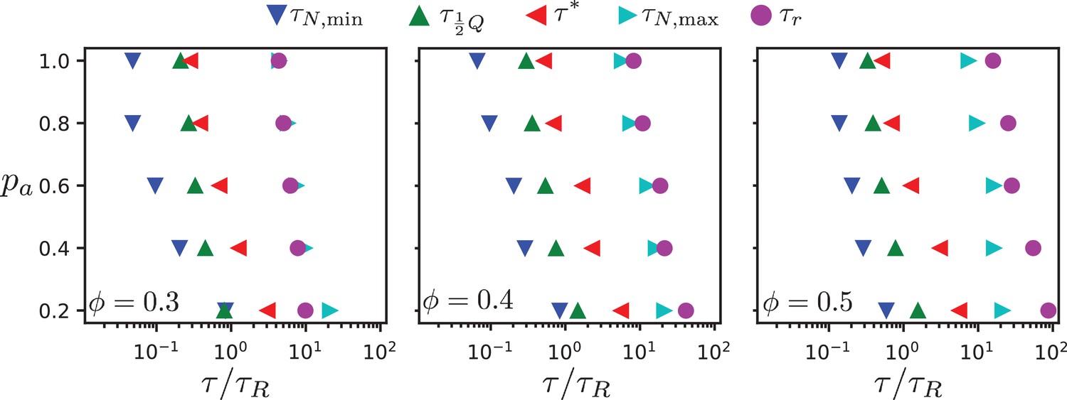
Table 1

Table of time scales involved in MT dynamics.

The time scales reported are approximate values for various antialigned motor probabilities $p_{a}$ and surface fractions $ϕ$ .

https://doi.org/10.7554/eLife.39694.039

	Symbols	Time scale ( $τ_{R}$ )	Derivation
Passive diffusion	$τ_{D}$	$τ < 10^{- 1}$	Slope of MSD $\approx 1$
Antialigned propulsion	$τ_{N, \min}$	$τ \approx 10^{- 1}$	Minimum of $N_{d}$
Streaming	$τ_{Q / 2}$	$10^{- 1} < τ < 10^{0}$	$⟨ ψ_{i} ⟩$ decay time
Maximal skew	$τ^{*}$	$10^{0} < τ < 10^{1}$	Maximum skew of $𝐩_{0} \cdot 𝐝$
Collective migration	$τ_{N, \max}$	$τ \approx 10^{1}$	Maximum of $N_{d}$
Active rotation	$τ_{r}$	$τ > 10^{1}$	Orientational correlation time

Table 2

Parameter values used in the simulations.

https://doi.org/10.7554/eLife.39694.040

Parameter	Symbol	Value	Notes/Biological Values
Thermal energy	$k_{B} T$	$4.11 pN nm$	room temperature
MT length	$L$	$0.625$ $μ$ m	$2.5 \pm 1.4$ $μ$ m (Howard et al., 1989)
MT diameter	$σ$	$25$ nm	(Chrétien and Wade, 1991)
MT bond angle constant	$κ$	$2.055 \times 10^{4} pN {nm}^{2}$	rigid MTs
MT bond spring constant	$k_{s}$	$13.15 pN / nm$	preserves MT length (Isele-Holder et al., 2015)
Dynamic viscosity	$η$	$1$ Pa s	viscosity of cytoplasm (Wirtz, 2009)
Characteristic energyof WCA potential	$ϵ$	$4.11$ pN nm	(Bates and Frenkel, 2000; Bolhuis and Frenkel, 1997; McGrother et al., 1996)
Motor spring constant	$k_{m}$	$6.6 \times 10^{- 3}$ pN/nm	$0.33 pN / nm$ per kinesin (Coppin et al., 1995), high number of effective motors
Equilibrium motor length	$d_{eq}$	$25$ nm	MT-MT distance at contact
Motor dwell time	$δ t$	$4.16 \times 10^{- 4}$ s

Table 3

Dimensionless parameters and ranges of the values used in the simulations.

https://doi.org/10.7554/eLife.39694.041

Parameter	Symbol	Value
MT surface fraction	$ϕ$	$0.2 - 0.5$
MT aspect ratio	$L / σ$	$10$
Reduced MT bond angle stiffness	$κ σ / k_{B} T$	$200$
Reduced MT persistence length	$ℓ_{p} / L$	$200$
MT bond spring constant	$k_{s} σ^{2} / k_{B} T$	$2000$
Reduced motor spring constant	$k_{m} σ^{2} / k_{B} T$	$1$
Reduced motor equilibrium length	$d_{eq} / σ$	$1$
Antialigned motor probability	$p_{a}$	$0 - 1.0$
Reduced single-bead friction	$γ / (k_{m} δ t)$	$171.6$
Reduced system size	$L_{b} / L$	$16 - 25$

Additional files

Source code file 1 Source code that adds effective motors to simulations of semiflexible filaments using the open-source Large-scale Atomic/Molecular Massively Parallel Simulator (LAMMPS).: https://doi.org/10.7554/eLife.39694.042
Download elife-39694-code-v2.zip
Transparent reporting form: https://doi.org/10.7554/eLife.39694.043
Download elife-39694-transrepform-v2.pdf

Download links

A two-part list of links to download the article, or parts of the article, in various formats.

Downloads (link to download the article as PDF)

Open citations (links to open the citations from this article in various online reference manager services)

Mendeley

Cite this article (links to download the citations from this article in formats compatible with various reference manager tools)

Arvind Ravichandran
Özer Duman
Masoud Hoore
Guglielmo Saggiorato
Gerard A Vliegenthart
Thorsten Auth
Gerhard Gompper

(2019)

Chronology of motor-mediated microtubule streaming

eLife 8:e39694.

https://doi.org/10.7554/eLife.39694

Share this article

Cite this article

Schematic illustrating MT bundling and streaming.

Schematic explaining the conditions that satisfy the antialigned motor potential.

Motor-driven and diffusive motion of MTs.

Figure 3—source data 1

Parallel velocity v∥, extrapolated to τ=0 as function of the antialigned motor probability pa for various MT surface fractions ϕ.

Simulation snapshots at steady state for various antialigned motor probabilities pa and MT surface fractions ϕ.

Translational MT mean squared displacements for various antialigned motor probilities pa and MT surface fractions ϕ.

Parallel velocity v∥ as a function of the time window τ for various antialigned motor probabilities pa and MT surface fractions ϕ.

Maximum parallel MT velocities v∥,A⁢(τ*) as function of the antialigned motor probability pa for various MT surface fractions ϕ.

Histogram of v∥ for various MT surface fractions ϕ and five time windows τ.

Histogram of v∥⁢(τ*) for various pa and ϕ.

Probability densities of the MT local polar order parameter ψi.

MT parallel velocity distributions.

MT mean squared displacements: computer simulation and experimental data.

Displacement correlations of MTs.

Figure 4—source data 1

Neighbour displacement correlation function Nd⁢(τ) for various MT surface fractions ϕ and antialigned motor probabilities pa.

Local polar order of MTs.

Figure 5—source data 1

MTs coloured based on their local polar order parameter ψi for pa=1.0, ϕ=1.0.

Deviation from local polar order Q⁢(τ) as function of the lag time τ for various antialigned motor probabilities pa for polar-aligned MTs.

Mean local polar order parameter of MTs at long times, ⟨ψ∞⟩, for various surface fractions ϕ and antialigned motor probabilities pa.

MT parallel velocity distributions.

Figure 6—source data 1

Skews α3 of parallel velocity distributions (v∥) (Fig.

Ratios of MT populations in environments with different local polar order.

First three moments of the parallel velocity (v∥) distribution.

Collective motion of MTs.

FRAP-like predictions for various MT surface fractions ϕ.

MT orientational correlation and active diffusion.

Figure 8—source data 1

Chronology of MT streaming. Events from antialigned MT propulsion to MT rotation (left to right) which make up the streaming process, for various antialigned motor probabilities pa and surface fractions ϕ=0.3, ϕ=0.4, and (c) ϕ=0.5 as indicated.

Figure 9—source data 1

Mean squared displacements of filaments obtained from Langevin Dynamics (LD) and Brownian Dynamics (BD), for single filaments (left) and filaments in suspensions with packing fraction 𝜙 = 0.3 (right).

Steady-state dynamics of the MT-effective motor system shown in Figure 3(a) for 100 τR.

Streaming motion of antialigned and diffusive motion of polar-aligned MTs for 100 τR, corresponding to Figure 3(b). The scale bar corresponds to the length of 10 MTs.

Center-of-mass trajectories for selected MTs for 300⁢τR, corresponding to Figure 3(c).

Inhomogeneous dynamics over a period of 100 τR.

Table of time scales involved in MT dynamics.

Parameter values used in the simulations.

Dimensionless parameters and ranges of the values used in the simulations.

Source code file 1

Transparent reporting form

Downloads (link to download the article as PDF)

Open citations (links to open the citations from this article in various online reference manager services)

Cite this article (links to download the citations from this article in formats compatible with various reference manager tools)

Parallel velocity $v_{∥}$ , extrapolated to $τ = 0$ as function of the antialigned motor probability $p_{a}$ for various MT surface fractions $ϕ$ .

Simulation snapshots at steady state for various antialigned motor probabilities $p_{a}$ and MT surface fractions $ϕ$ .

Translational MT mean squared displacements for various antialigned motor probilities $p_{a}$ and MT surface fractions $ϕ$ .

Parallel velocity $v_{∥}$ as a function of the time window $τ$ for various antialigned motor probabilities $p_{a}$ and MT surface fractions $ϕ$ .

Maximum parallel MT velocities $v_{∥, A} (τ^{*})$ as function of the antialigned motor probability $p_{a}$ for various MT surface fractions $ϕ$ .

Histogram of $v_{∥}$ for various MT surface fractions $ϕ$ and five time windows $τ$ .

Histogram of $v_{∥} (τ^{*})$ for various $p_{a}$ and $ϕ$ .

Probability densities of the MT local polar order parameter $ψ_{i}$ .

Neighbour displacement correlation function $N_{d} (τ)$ for various MT surface fractions $ϕ$ and antialigned motor probabilities $p_{a}$ .

MTs coloured based on their local polar order parameter $ψ_{i}$ for $p_{a} = 1.0$ , $ϕ = 1.0$ .

Deviation from local polar order $Q (τ)$ as function of the lag time $τ$ for various antialigned motor probabilities $p_{a}$ for polar-aligned MTs.

Mean local polar order parameter of MTs at long times, $⟨ ψ_{\infty} ⟩$ , for various surface fractions $ϕ$ and antialigned motor probabilities $p_{a}$ .

Skews $α_{3}$ of parallel velocity distributions ( $v_{∥}$ ) (Fig.

First three moments of the parallel velocity ( $v_{∥}$ ) distribution.

FRAP-like predictions for various MT surface fractions $ϕ$ .

Chronology of MT streaming. Events from antialigned MT propulsion to MT rotation (left to right) which make up the streaming process, for various antialigned motor probabilities $p_{a}$ and surface fractions $ϕ = 0.3$ , $ϕ = 0.4$ , and (c) $ϕ = 0.5$ as indicated.

Steady-state dynamics of the MT-effective motor system shown in Figure 3(a) for 100 $τ_{R}$ .

Streaming motion of antialigned and diffusive motion of polar-aligned MTs for 100 $τ_{R}$ , corresponding to Figure 3(b). The scale bar corresponds to the length of 10 MTs.

Center-of-mass trajectories for selected MTs for $300 τ_{R}$ , corresponding to Figure 3(c).

Inhomogeneous dynamics over a period of 100 $τ_{R}$ .