NetPyNE, a tool for data-driven multiscale modeling of brain circuits
- State University of New York Downstate Medical Center, United States
- Northwestern University, United States
- University College London, United Kingdom
- MetaCell LLC, United States
- EyeSeeTea Ltd, United Kingdom
- University of Sydney, Australia
- Nathan Kline Institute for Psychiatric Research, United States
- Yale University, United States
- Kings County Hospital, United States
Figures
Figure 1
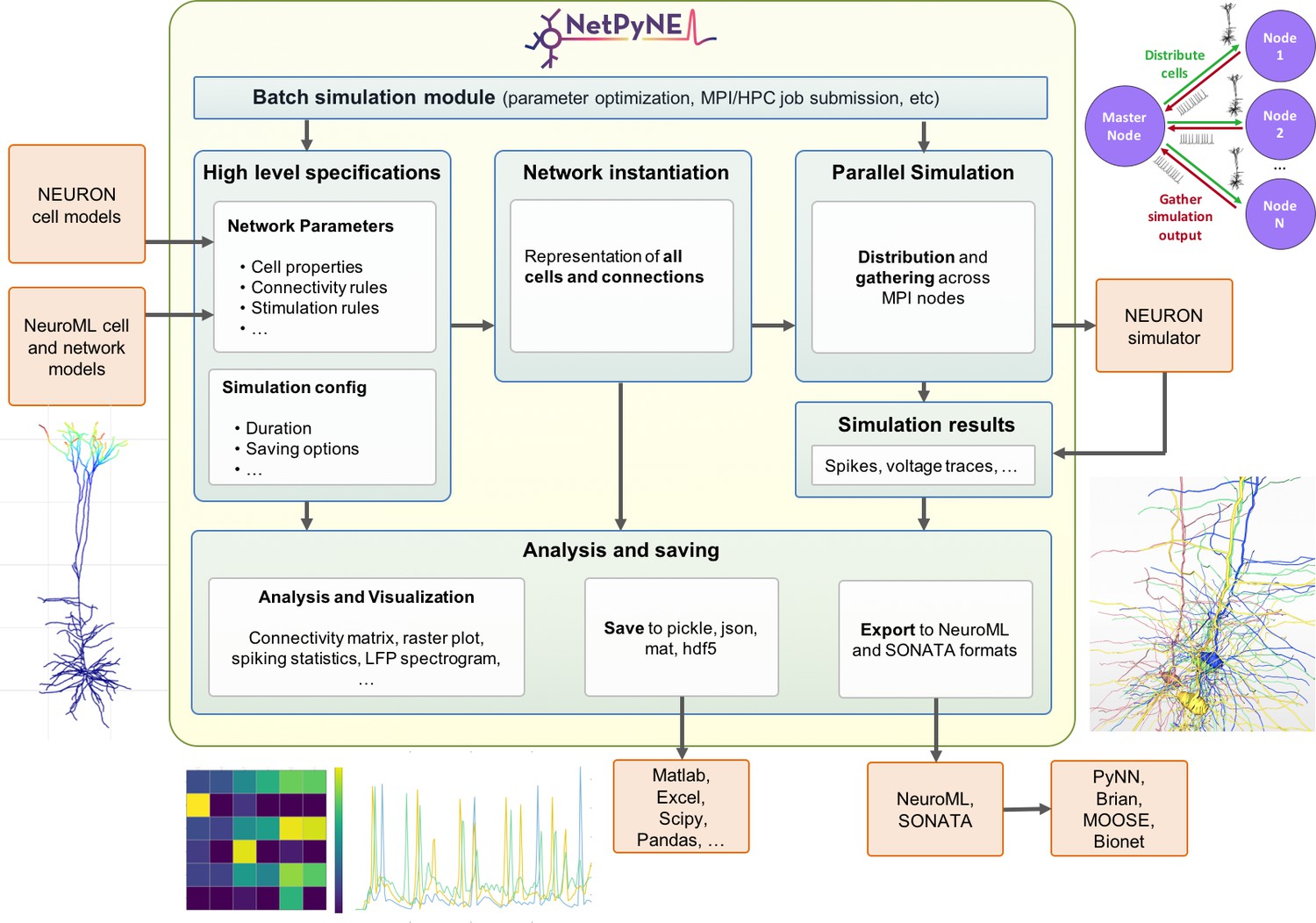
Overview of NetPyNE components and workflow.
Users start by specifying the network parameters and simulation configuration using a high-level JSON-like format. Existing NEURON and NeuroML models can be imported. Next, a NEURON network model is instantiated based on these specifications. This model can be simulated in parallel using NEURON as the underlying simulation engine. Simulation results are gathered in the master node. Finally, the user can analyze the network and simulation results using a variety of plots; save to multiple formats or export to NeuroML. The Batch Simulation module enables automating this process to run multiple simulations on HPCs and explore a range of parameter values.
Figure 2
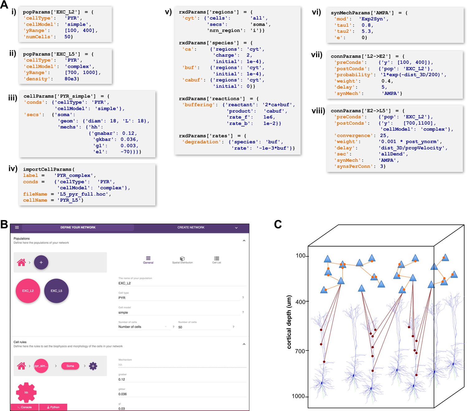
High-level specification of network parameters.
(A) Programmatic parameter specification using standardized declarative JSON-like format. i,ii: specification of two populations iii,iv: cell parameters; v: reaction-diffusion parameters; vi,vii,viii: synapse parameters and connectivity rules. (B) GUI-based parameter specification, showing the definition of populations equivalent to those in panel A. (C) Schematic of network model resulting from the specifications in A.
Figure 3
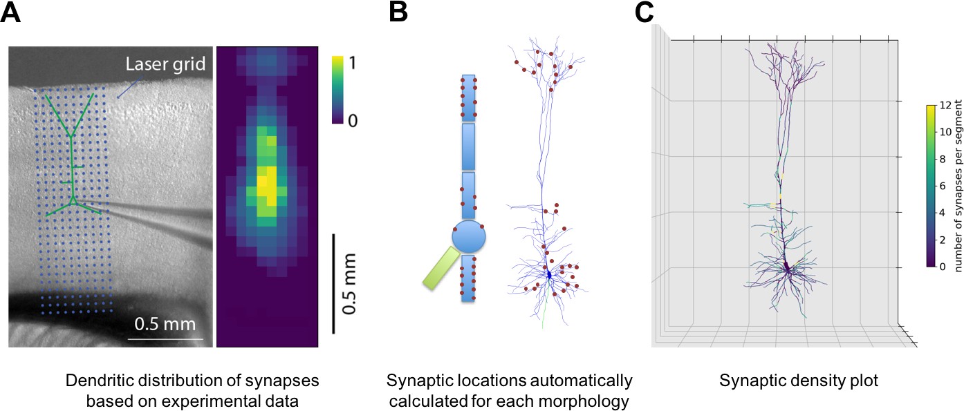
Specification of dendritic distribution of synapses.
(A) Optogenetic data provides synapse density across the 2D grid shown at left (Suter and Shepherd, 2015). (B) Data are imported directly into NetPyNE which automatically calculates synapse location in simplified or full multicompartmental representations of a pyramidal cell. (C) Corresponding synaptic density plot generated by NetPyNE.
Figure 4
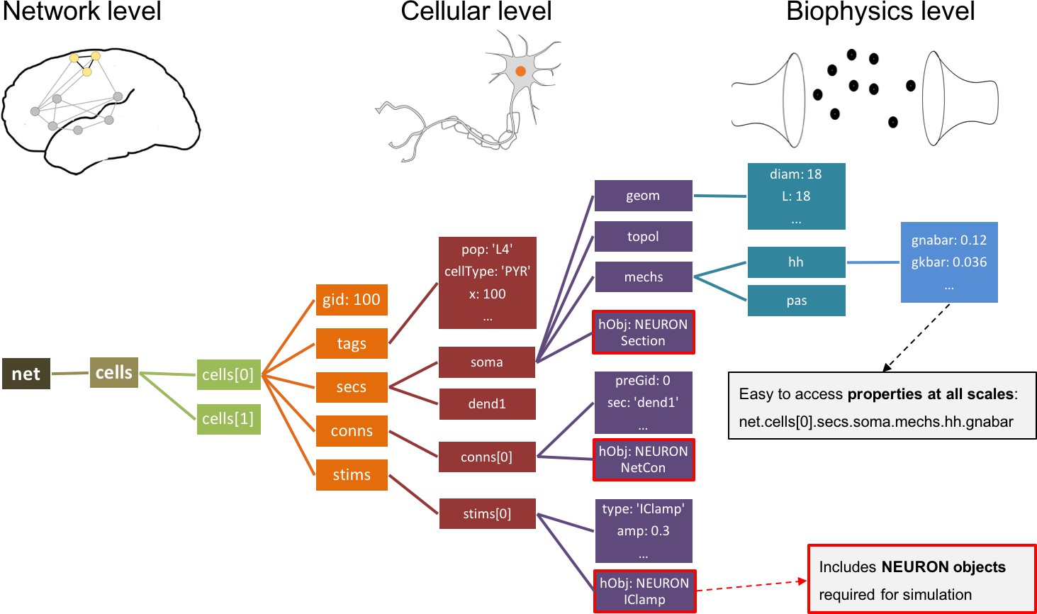
Instantiated network hierarchical data model.
The instantiated network is represented using a standardized hierarchically organized Python structure generated from NetPyNE ’s high-level specifications. This data structure provides direct access to all elements, state variables and parameters to be simulated. Defined NEURON simulator objects (represented as boxes with red borders) are included within the Python data structure.
Figure 5
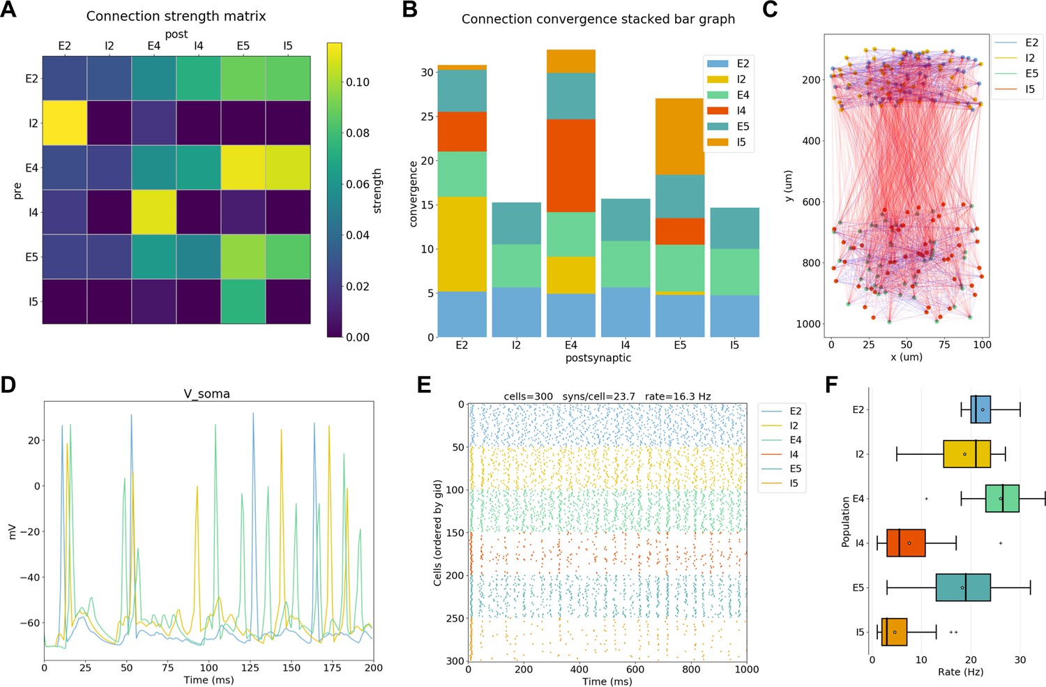
NetPyNE visualization and analysis plots for a simple three-layer network example.
(A) Connectivity matrix, (B) stacked bar graph, (C) 2D graph representation of cells and connections, (D) voltage traces of three cells, (E) spike raster plot, (F) population firing rate statistics (boxplot).
Figure 6

LFP recording and analysis.
(A) LFP signals (left) from 10 extracellular recording electrodes located around a morphologically detailed cell (right) producing a single action potential (top-right). (B) LFP signals, PSDs and spectrograms (left and center) from four extracellular recording electrodes located at different depths of a network of 120 five-compartment neurons (right) producing oscillatory activity (top-left).
Figure 7
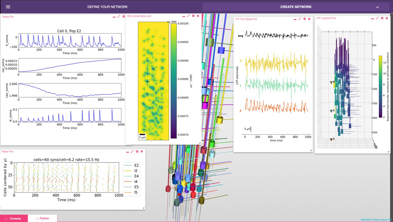
NetPyNE graphical user interface (GUI) showing a multiscale model.
Background shows 3D representation of example network with 6 populations of multi-channel, multi-compartment neurons; results panels from left to right: singe-neuron traces (voltage, intracellular and extracellular calcium concentration, and potassium current); spike raster plot; extracellular potassium concentration; LFP signals recorded from three electrodes; and 3D location of the LFP electrodes within network.
Figure 8
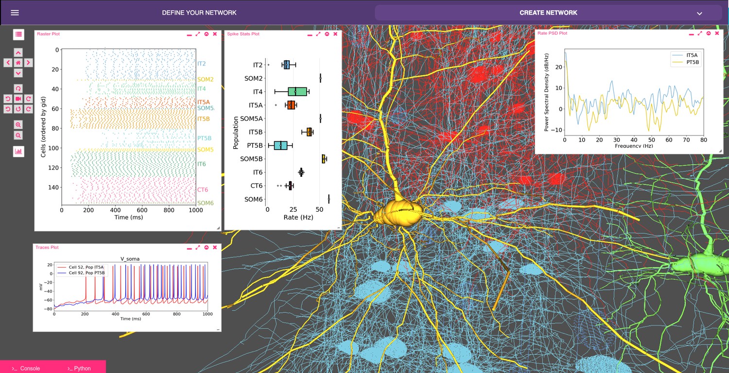
Model of M1 microcircuits developed using NetPyNE (scaled down version).
NetPyNE GUI showing 3D representation of M1 network (background), spike raster plot and population firing rate statistics (top left), voltage traces (bottom left) and firing rate power spectral density (top right).
Figure 9
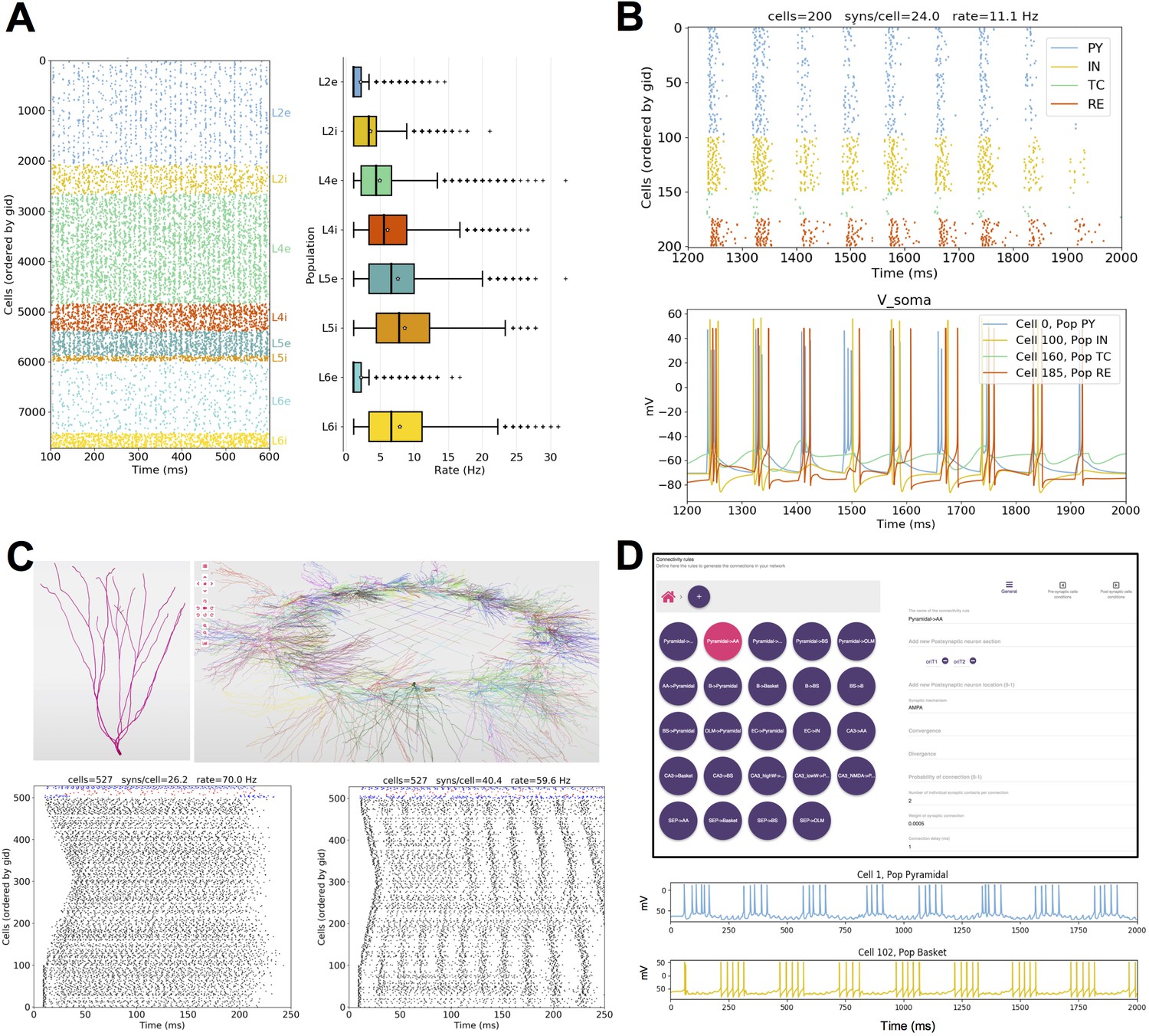
Published models converted to NetPyNE.
All figures were generated using the NetPyNE version of the models. (A) Spike raster plot and boxplot statistics of the Potjans and Diesmann thalamocortical network originally implemented in NEST (Potjans and Diesmann, 2014; Romaro et al., 2018). (B) Spike raster plot and voltage traces of a thalamocortical network exhibiting epileptic activity originally implemented in NEURON/hoc (Knox et al., 2018). (C) 3D representation of the cell types and network topology, and spike raster plots of a dentate gyrus model originally implemented in NEURON/hoc (Rodriguez, 2018; Tejada et al., 2014). (D) Connectivity rules (top) and voltage traces of 2 cell types (bottom) in a hippocampal CA1 model originally implemented in NEURON/hoc (Cutsuridis et al., 2010; Tepper et al., 2018).
Tables
Table 1
Number of lines of code in the original models and the NetPyNE reimplementations.
https://doi.org/10.7554/eLife.44494.012| Model description (reference) | Original language | Original num lines | NetPyNE num lines |
|---|---|---|---|
| Dentate gyrus (Tejada et al., 2014) | NEURON/hoc | 1029 | 261 |
| CA1 microcircuits (Cutsuridis et al., 2010) | NEURON/hoc | 642 | 306 |
| Epilepsy in thalamo (Knox et al., 2018) | NEURON/hoc | 556 | 201 |
| EEG and MEG in cortex/HNN model (Jones et al., 2009) | NEURON/Python | 2288 | 924 |
| Motor cortex with RL (Dura-Bernal et al., 2017) | NEURON/Python | 1171 | 362 |
| Cortical microcircuits (Potjans and Diesmann, 2014) | PyNEST | 689 | 198 |
Additional files
-
Transparent reporting form
- https://doi.org/10.7554/eLife.44494.013
Download links
A two-part list of links to download the article, or parts of the article, in various formats.
Downloads (link to download the article as PDF)
Open citations (links to open the citations from this article in various online reference manager services)
Cite this article (links to download the citations from this article in formats compatible with various reference manager tools)
NetPyNE, a tool for data-driven multiscale modeling of brain circuits
eLife 8:e44494.
https://doi.org/10.7554/eLife.44494


