MagC, magnetic collection of ultrathin sections for volumetric correlative light and electron microscopy
- University of Zurich and ETH Zurich, Switzerland
Figures
Figure 1 with 5 supplements
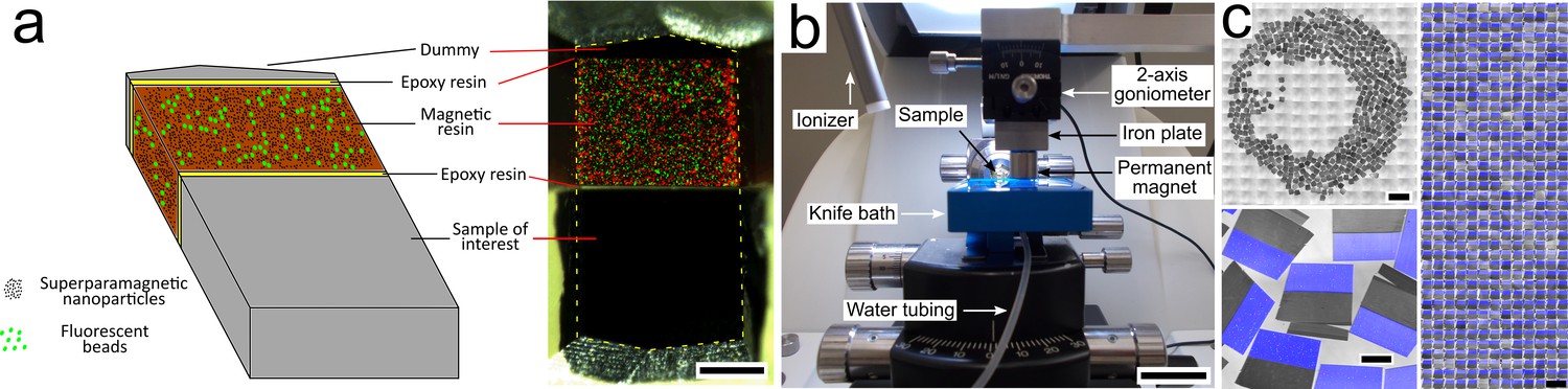
Magnetic augmentation and collection of sections on silicon wafer.
(a) Augmentation of a polymerized sample block with resin containing superparamagnetic nanoparticles (for remote magnetic actuation) and fluorescent beads (for section order retrieval). (b) Setup for MagC: a diamond knife with a large bath and a mobile overhanging magnet. (c) 507 consecutive ultrathin sections collected on a silicon wafer: wafer overview, close-up (merge of whitefield and three fluorescent channels: blue for coumarin stain, plus green- and red-fluorescent beads) and montage of all sections. Scale bars: (a) 200 μm; (b) 2 cm; (c) 2 mm (top left), 200 μm (bottom left), 1 mm (right).
Figure 1—figure supplement 1
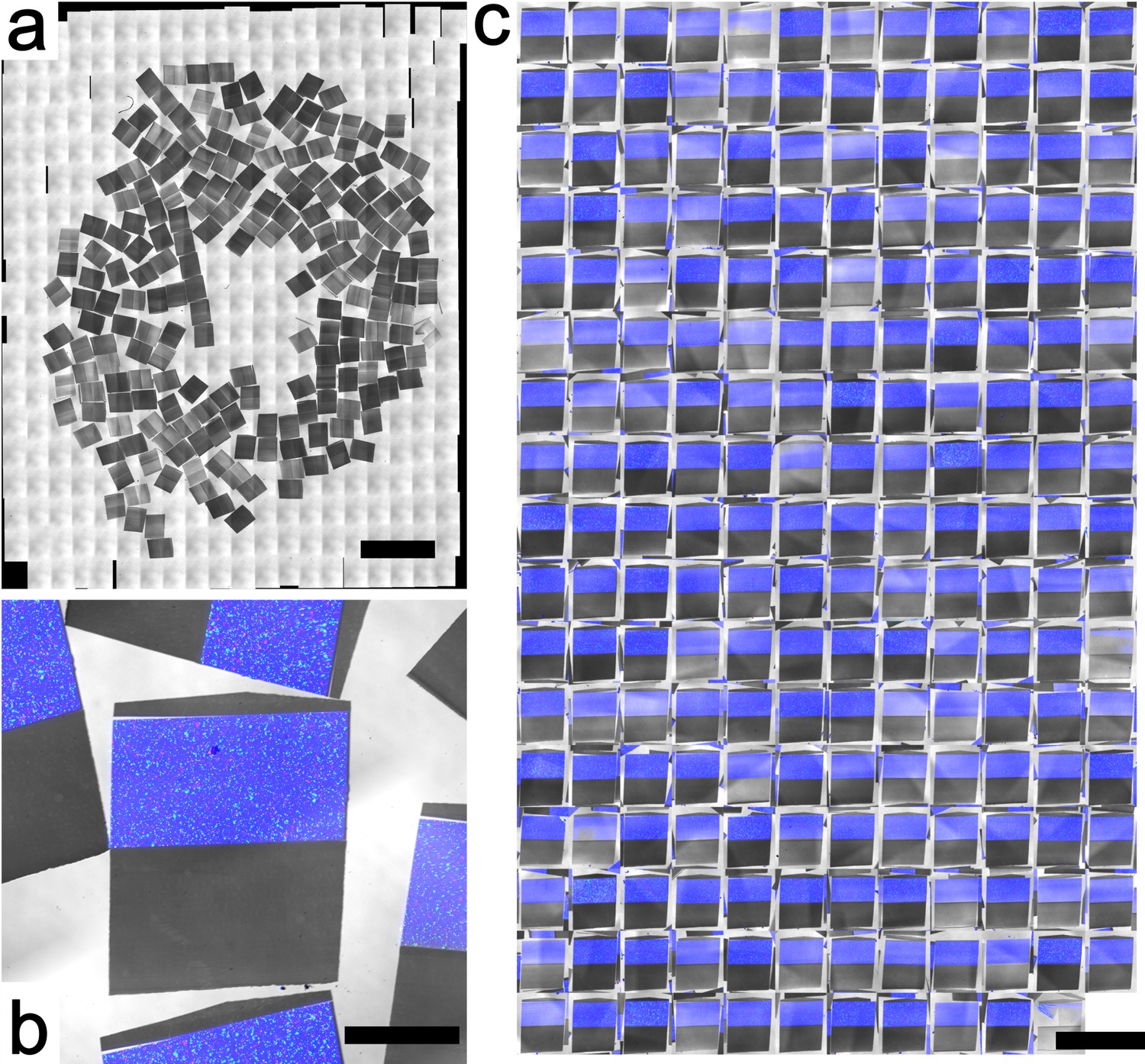
Wafer overview for Dataset 2.
(a) Widefield LM of the collected sections. The intensity differences come from section thickness inhomogeneity. As documented by Harris et al. (2006) , the lack of an hermetic enclosure during sectioning typically induces section inhomogeneity. (b) Close-up around one section, showing merged multichannel fluorescent imagery: blue for Coumarin, with green- and red-fluorescent beads. (c) Montage of all sections with the same orientation. Scale bars: (a) 4 mm; (b) 500 μm; (c) 2 mm.
Figure 1—figure supplement 2

Electron micrographs of the sections for Dataset 1.
(a) Electron micrograph of numerous sections collected on wafer. Most of the collected sections exhibit a dummy (like that highlighted in the yellow box) that is attached to their tissue part and that comes from the previous section, which is explained by the following mechanism: with this sample block, the dummy part often detached from the section during sectioning or immediately after landing on the water surface. The main part (magnetic resin and tissue) of the last cut section was then floating freely while its dummy remained attached to the edge. Then the main part of the next cut section stuck to the previous dummy and so on. (b) EM of a section. The yellow dashed square highlights the region that has been imaged with the electron microscope and became darker due to the beam irradiation. (c) EM of well-dispersed superparamagnetic nanoparticles in the appended resin. (d) Small contaminations with the appearance of oily droplet can sometimes be found in the magnetic resin. These could be unreacted oleic acids, an oily compound from handling during preparation, or something unknown to the author. Scale bars: (a) 1 mm; (b) 100 µm; (c) 500 nm; (d) 2 µm.
Figure 1—figure supplement 3

Magnetic augmentation.
(a) Mounting helper device. The manual manipulator allows the experimenter to precisely place the needle in contact with the block to be glued onto the sample. The iron plate together with the base magnet of the needle holder maintain the position set by the manipulator. (b) The detachable part is placed in an oven for temperature curing. (c) The biological sample is trimmed manually with a razor blade. (d) The magnetic resin is glued to the sample and maintained in place with a needle. (e) Overlay of color and fluorescent imagery showing the fluorescent particles contained in the magnetic resin. (f) The magnetic resin is manually trimmed down to achieve roughly a 50/50 ratio of sample surface to magnetic surface suitable for sectioning at 50 nm nominal thickness. (g) An additional dummy piece of heavy-metal-stained brain tissue embedded in resin is glued to the block. Scale bars: (a, b) 20 mm; (c–g): 500 μm.
Figure 1—figure supplement 4
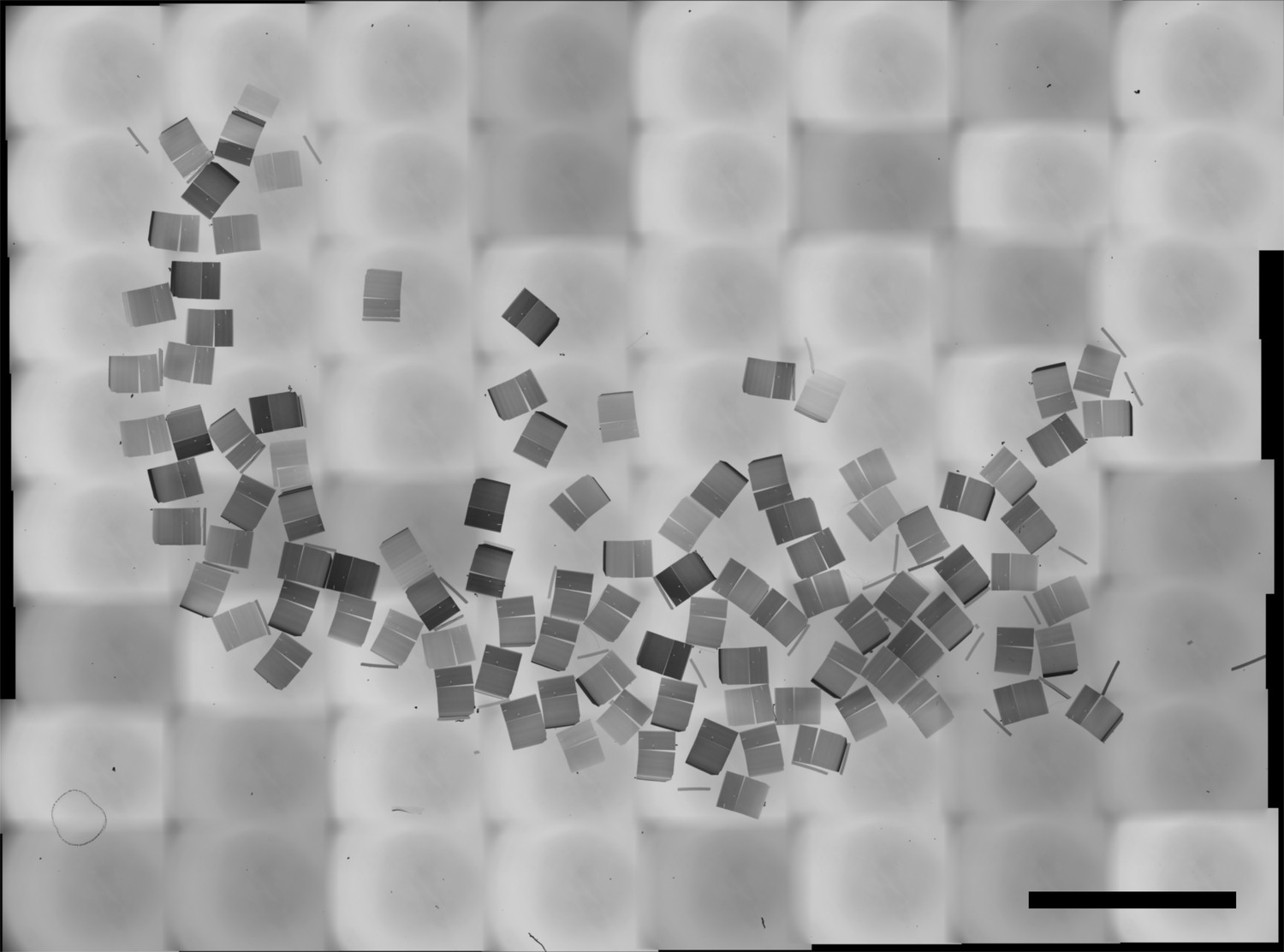
Wafer overview of the 100 sections collected during the video-recorded session.
Scale bar: 5 mm.
Figure 1—figure supplement 5

Multibeam scanning EM of magnetically collected sections on silicon wafer.
(a) Overview of the 15 consecutive sections collected with MagC that were used for the first MultiSEM experiment. (b) Overview of 91 stitched tiles. (c) A tile produced by one of the 91 beams. The image quality is representative of the quality observed in the whole section. (d) An inset from a tile acquired with a Zeiss MultiSEM of a section from Dataset 1 after the complete CLEM pipeline and an additional wafer-wide broad ion beam milling of about 25 nm (Templier, in preparation). Imaging conditions: silicon wafer chip glued to the EM stub with carbon glue, 4 nm pixel size, 400 ns dwell time, Scale bars: (a) 2 mm; (b) 20 μm; c) 2 μm; d) 1 μm.
Figure 2 with 6 supplements
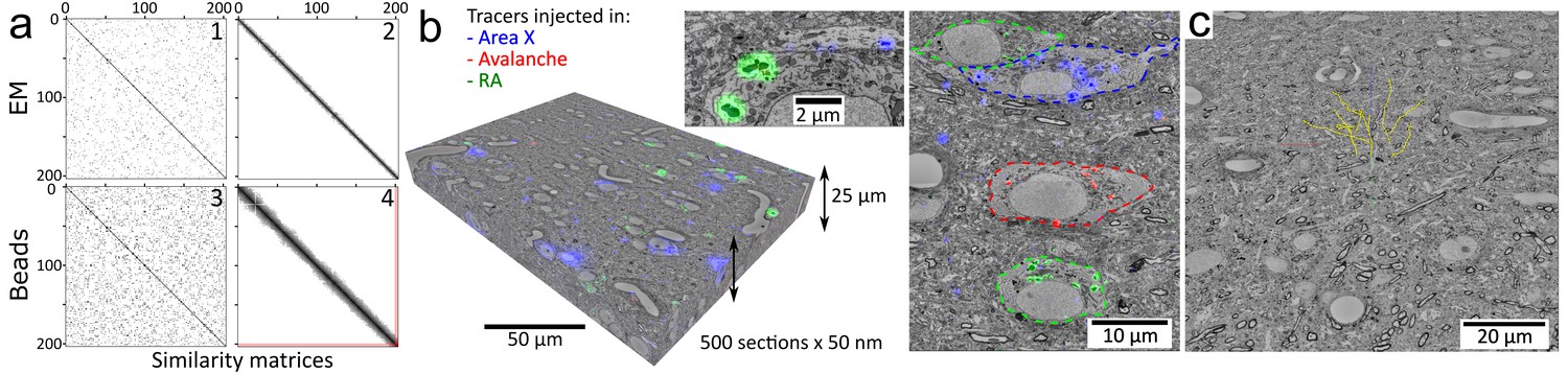
Volumetric correlative LM-EM with MagC collected sections.Volumetric correlative LM-EM with MagC collected sections.
(a) Section-order retrieval for Dataset 2 (1% fluorescent beads) obtained with EM imagery (panels 1 and 2 show the pairwise similarity matrices before and after reordering, respectively) and with fluorescent beads imagery (panels 3 and 4). Darker pixels depict higher similarity whereas white pixels depict no similarity. The two red lines in panel 4 indicate a single flip in the computed order that was later corrected with EM imagery. (b) Volumetric correlative stack for Dataset 1 with three fluorescent channels and 507 consecutive ultrathin sections. Insets: close-ups of cell bodies and a neurite carrying different neuroanatomical tracers. The cell bodies in the right panel are outlined with colored dashed lines. Blue: tracer injected into Area X. Green: tracer injected into the nucleus Robustus of the arcopallium (RA). Red: tracer injected into Avalanche. (c) The EM imagery was connectomics-grade and enabled neurite tracing. Yellow dots: skeletons stemming from nine seed points placed in a 3×3 grid in the first section of Dataset 2.
Figure 2—figure supplement 1
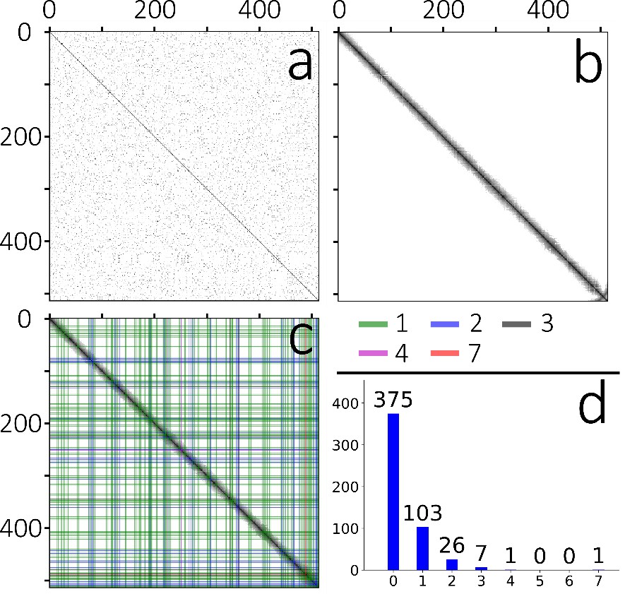
Section order retrieval for Dataset 1 (low concentration of beads).
(a) Matrix of pairwise similarities of unordered sections computed with EM imagery. Darker pixels depict higher similarity whereas white pixels depict no similarity. (b) Reordered EM matrix. (c) Matrix of pairwise similarities of unordered sections computed with fluorescent bead imagery. The original order is the order provided by the section segmentation pipeline. (d) Similarity matrix of the reordered sections. The order overall looks to be consistent, except for slight deviations at the end of the dataset (around section number 500) that can be seen in the lower left of the matrix.
Figure 2—figure supplement 2
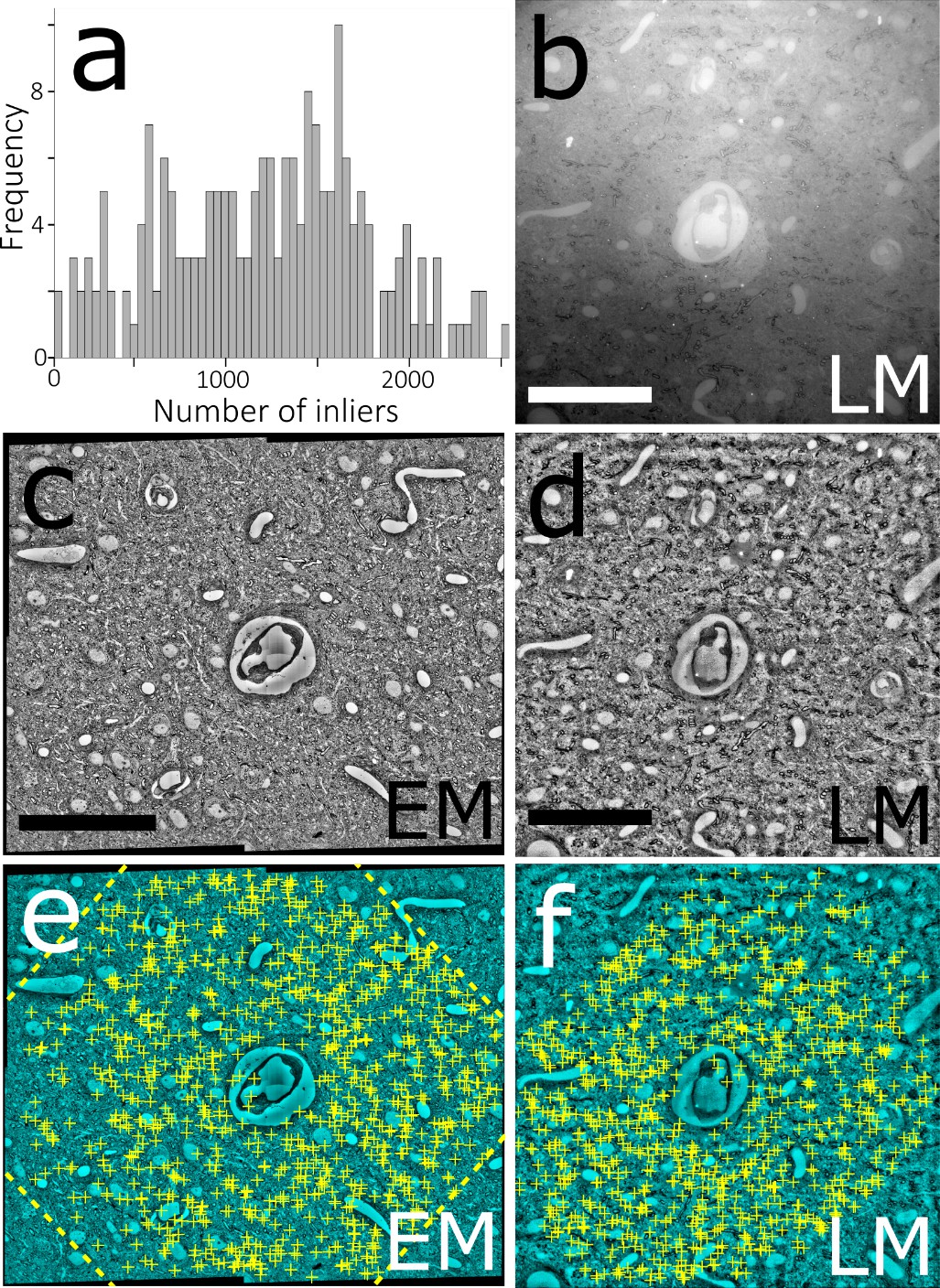
Automated LM-EM registration.
(a) Histogram of the numbers of matching inliers found for each of the 203 LM-EM pairs of Dataset 2. (b) A reflection brightfield light micrograph after simple thresholding. (c) Downscaled EM mosaic. (d) Same micrograph as in (a) after local contrast normalization. Note the high similarity with its EM counterpart micrograph in (c). (e, f) Same micrographs as in (c) and (d), respectively. The yellow crosses show the locations of SIFT features that match between the two images. The dashed yellow lines in (e) show the outline of the LM micrograph when affine transformed to match its EM counterpart. Scale bars: 50 μm.
Figure 2—figure supplement 3
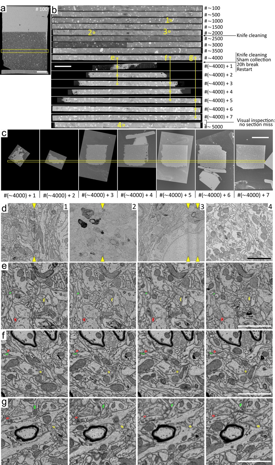
Sectioning quality and restart of a MagC block.All images are SEM micrographs of sections manually collected on a silicon wafer.
(a) Section number #100. The yellow box indicates the region acquired at high resolution for the sections up to number #~3500 (see panel (c) for sections above #4000). (b) Montage of the high-resolution regions acquired. The corresponding indices are shown on the right. The insets numbered 1 to 4 are shown in panel (d). Insets 1, 2 and 3 are the only locations where vertical streaks resulting from sectioning were found. Inset 4 in section #~5000 is representative of the streak-free sectioning quality manually observed in all acquired high-resolution regions. The insets illustrating restart continuity (labeled e, f, and g) are shown below in panels with corresponding lettering. (c) Complete or partial sections collected after the restart. The yellow box shows the region acquired in section numbers above #4000. The nature of the cuts was observed through the binocular microscope simultaneously during the sectioning restart and is as follows (#1 refers to #~4000 + 1 and so on): #1, partial tissue; #2, partial tissue; #3, partial tissue; #4, partial tissue connected with partial magnet; #5, partial tissue connected with partial magnet (but disconnected during manual pickup, the magnetic and dummy parts remained stuck to the bottom of section #6); #6, partial tissue with disconnected partial magnet (the tissue/ magnet separation occurred immediately upon sectioning); #7, full tissue connected with full magnet (but disconnected during manual pickup, the magnetic portion is visible immediately to the right of the section); #8 to #15, full normal sections (not collected). (d) Insets 1, 2 and 3 from panel (b) showing (with yellow arrows) the only vertical streaks found after manual inspection among the entire high-resolution imagery from panel (b). Inset 4 from section #~5000 shows a representative image of the lack of image quality impairment that might occur due to a potentially damaged knife. (e– g) Four consecutive insets from the restart sections shown in yellow in panel (b). The interior of three small neuronal processes are painted in red, green and blue. There is no issue in tracing fine processes across the 20 hr long restart. The good continuity in panels (e–g) indicates that no material was lost despite the partial sections. Scale bars: (a) 200 mm; (b) 100 mm; (c) 500 mm; (d–g) 2 mm.
Figure 2—figure supplement 4
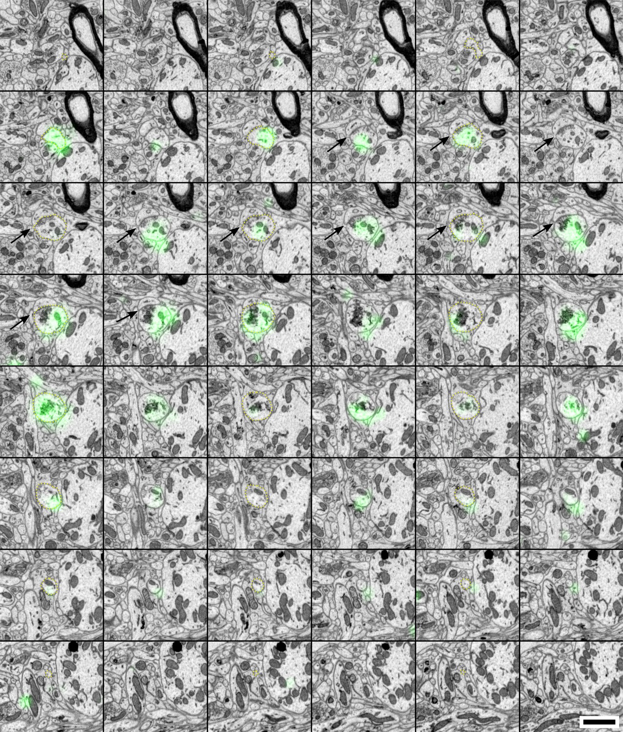
Labeled axon making a synapse en passant.
The axon is delineated with dashed yellow lines (every second section). Black arrows indicate the synapse. Scale bar: 1 µm.
Figure 2—figure supplement 5
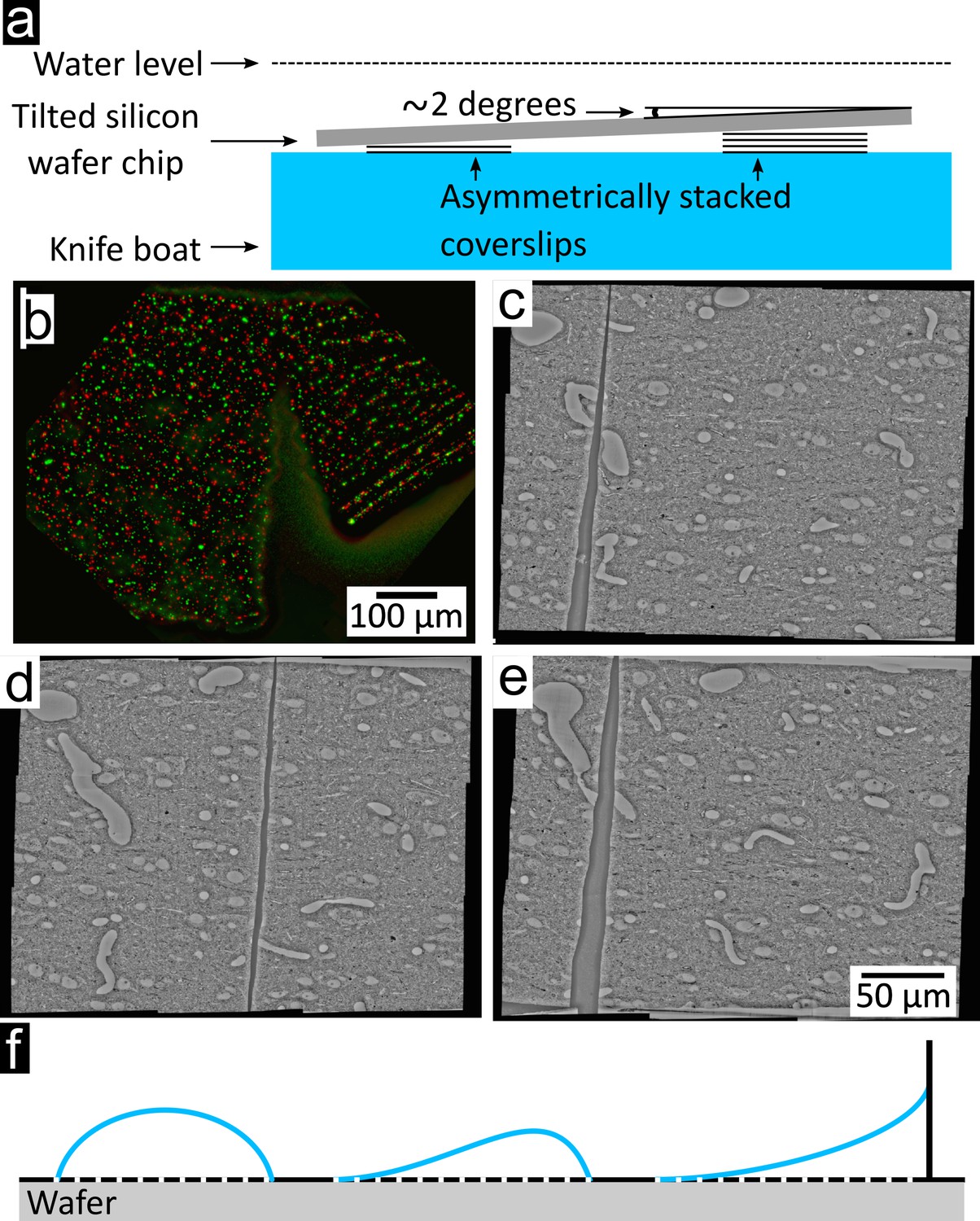
Section collection quality.
(a) Schematic of the immersed tilted silicon wafer chip. Side view from the experimenter looking towards the ultramicrotome (same point of view as in Figure 1b). A few microscopy coverslips are asymmetrically stacked to slightly tilt the wafer chip in order to avoid accumulation of water surface dust in the center of the wafer at the end of the water withdrawal. (b) The single tear found in Dataset 2, which was present in the magnetic portion of section #22. (c–e) tear in Dataset one in sections #258, #359 and #481, respectively. (f) Schematic of the interaction of water with a hydrophobic substrate, a partially hydrophobic substrate, and a substrate with nearby walls. All three configurations present a risk of impairing sections upon drying.
Figure 2—figure supplement 6

Multicolor correlative LM-EM imagery (Dataset 1) visualized in neuroglancer.
Multicolor correlative LM-EM imagery (Dataset 1) of zebra finch HVC nucleus showing three neuroanatomical tracers injected in Area X (blue), the nucleus Robustus of the Arcopallium (green), and Avalanche (red). The two panes on the right show x and y re-slices through the volume.
Videos
Video 1
Video-recorded magnetic collection.
Video available here: https://youtu.be/o13r-tHT9-c. Timeline:1. 00:02 - Ultramicrotome start, 2. 00:19 - Cutting ..., 3. 06:21 - Cutting stopped, 4. 06:32 - Removal of ionizer, 5. 07:02 - Magnet scanning ..., 6. 17:25 - Blowing away 2 sections from wall, 7. 20:42 - Blowing away 1 section from wall, 8. 27:15 - Water removal ..., 9. 31:33 - Heating ..., 10. 45:41 - Wafer pickup.
Video 2
Zoom on wafer of Dataset 2.
Video available here: https://youtu.be/UC8Zrl2Xud4.
Video 3
Flythrough in EM imagery of Dataset 2.
Video available here: https://youtu.be/VL0F9DkZVaQ and associated data available at https://neurodata.io/data/templier2019/.
Tables
Table 1
Coordinates of adult male zebra finch nuclei targeted with tracer injections.
https://doi.org/10.7554/eLife.45696.018| RA | AreaX | Avalanche | |
|---|---|---|---|
| Head angle (degrees) | 65 | 45 | 45 |
| Pipette angle (degrees) | 45 | -20 | 0 |
| Anterior-Posterior (mm) | 3 | 6.45* | 1.8 |
| Media-Lateral (mm) | 2.45 | 1.55 | 2 |
| Dorso-Ventral (mm) | 1.3 | 2.95 | 1.05 |
| *with a 0 degree pipette angle |
Table 2
Characteristics of the two presented datasets.
BDA: biotinylated dextran amines
| Dataset | Section number | Anatomical region | Tracer | Injection site | Primary antibody | Secondary antibody | EM size (μm x μm) | EM dwell time (ns) | Pixel size (nm) |
|---|---|---|---|---|---|---|---|---|---|
| 1 | 507 | HVC | Alexa 488FITCTexas red | RAAreaXAvalanche | Rat anti-488Mouse anti-FITCGoat anti-rhodamine | 488 anti-rat647 anti-mouse546 anti-rhodamine | 275 x 205 | 820 | 8 |
| 2 | 203 | Dorsal RA | BDA | Caudal RA | mouse anti-BDA | 647 anti-mouse | 185 x 140 | 6000 | 8 |
Table 3
Tracer-antibody library.
LT: Life Technologies. VL: Vector Laboratories. JI: Jackson Immunoresearch.
| Antigen | Alexa 488 LT #D-22910 | FITC LT #D-1820 | Texas Red LT #D-3328 | BDA LT #D-1956 |
|---|---|---|---|---|
| Antibody species | rabbit (LT #A-11094) rat (Biotem #custom) | mouse rabbit (LT #A-889) | goat (VL #SP-0602) | mouse (JI #200-002-211) |
Additional files
-
Transparent reporting form
- https://doi.org/10.7554/eLife.45696.021
Download links
A two-part list of links to download the article, or parts of the article, in various formats.
Downloads (link to download the article as PDF)
Open citations (links to open the citations from this article in various online reference manager services)
Cite this article (links to download the citations from this article in formats compatible with various reference manager tools)
MagC, magnetic collection of ultrathin sections for volumetric correlative light and electron microscopy
eLife 8:e45696.
https://doi.org/10.7554/eLife.45696


