Nanoresolution real-time 3D orbital tracking for studying mitochondrial trafficking in vertebrate axons in vivo
- Center for Nano Science (CENS), Center for Integrated Protein Science (CIPSM) and Nanosystems Initiative München (NIM), Ludwig Maximilians-Universität München, Germany
- Center for Integrated Protein Science (CIPSM), German Center for Neurodegenerative Diseases (DZNE), Institute of Neuronal Cell Biology, Technische Universität München, Germany
Figures
Figure 1 with 3 supplements
3D orbital tracking microscope and mitochondrial trajectory analysis.
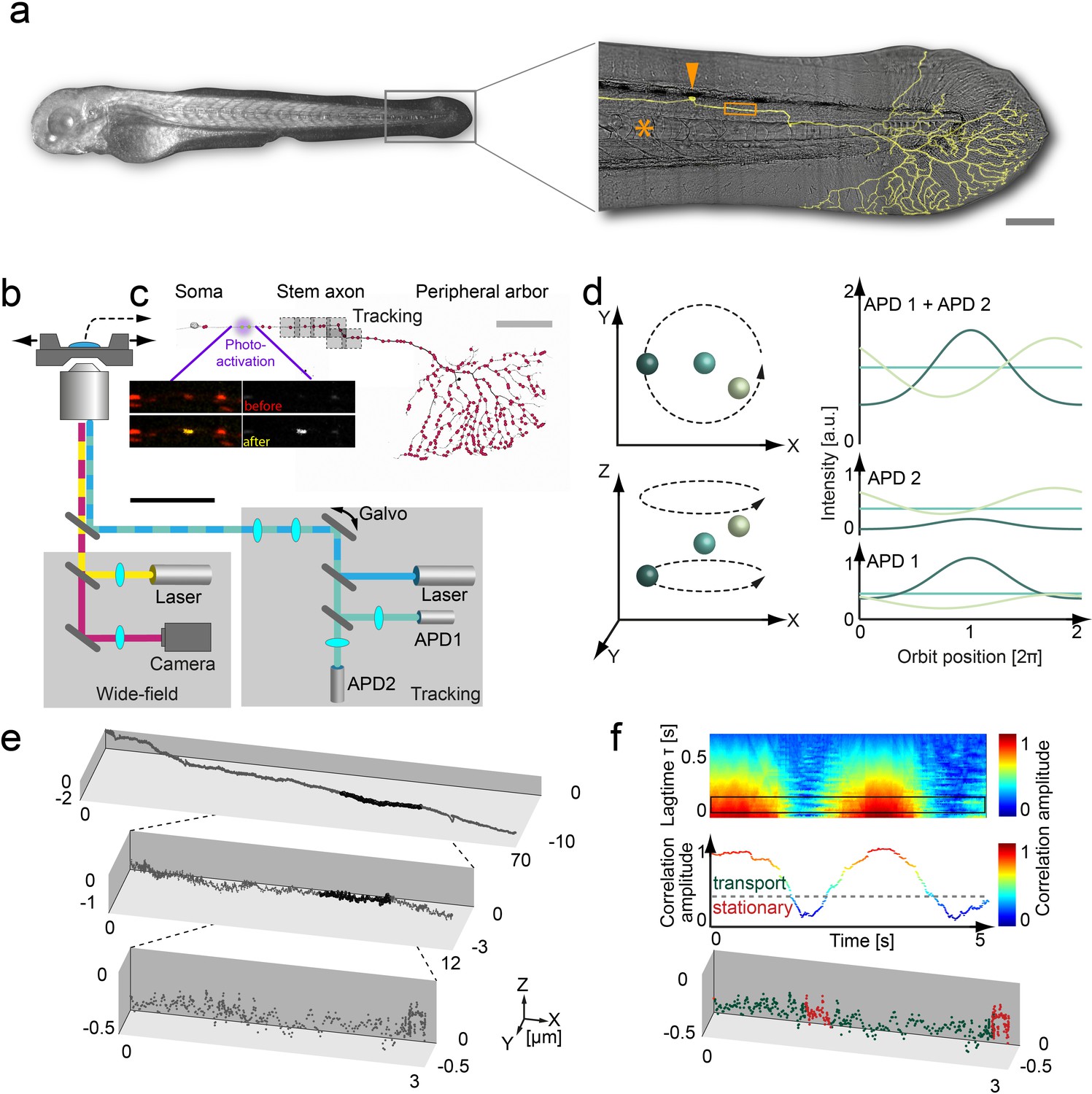
(a) Light microscopy transmission image of the zebrafish and a zoom in on the tail with a typical Rohon-Beard neuron labeled by a membrane-targeted fluorescent protein (shown in yellow). The typical tracking area (orange box), soma (orange arrow) and notochord (orange asterisks) are indicated to provide a contextual overview (scale bar, 200 μm). (b) Schematic of the custom-built 3D real-time orbital tracking microscope consisting of a confocal tracking channel and a wide-field channel for simultaneous environmental observation. (c) A confocal reconstruction of a sensory neuron is shown where both the membrane and the individual mitochondria, indicated schematically as red points, are fluorescently labeled (scale bar, 100 µm). The imaging sites in the stem axon are shown in gray with the multiple boxes indicating the re-location of the field of view during long-range tracking. Images of TagRFP (in red)/PA-GFP-labeled (in yellow) axonal mitochondria before (upper image pair) and after (lower image pair) photo-activation of a single mitochondrion are shown (scale bar, 5 µm). (d) Schematic representation of the 3D orbital tracking approach. Different particle locations are indicated through spheres of varying color. Lateral localization is performed by orbiting the laser focus around the particle of interest (top left). The amplitude and peak position of the intensity orbit depends on the position of the particle in relation to the center of the orbit (top right). The color of the line represents the signal coming from the object of the corresponding color in the left panels. The axial localization is achieved by using two confocal detection volumes placed equidistant above and below the focal plane (bottom left), so the intensity ratio between the two planes is proportional to the axial position of the particle (bottom right). (e) A trajectory of an anterograde moving mitochondrion (100 Hz, 20,000 data points). Zoom-ins illustrate the actual density of the acquired data points. (f) Autocorrelation carpet (top) of the angle between consecutive orbits. The black box indicates the lag time τ region averaged for the plot shown in the middle panel. Dashed line marks the threshold that was used to separate stationary phases (red points in bottom panel) from directed motion (green data points) in the lower plot. The lower plot is the same as shown in the maximum zoom-in in panel e). Galvo: galvanometer mirrors; APD, avalanche photodiode.
-
Figure 1—source data 1
Matlab files for analyzing and producing graphics of trajectory from panel e and correlation analysis from panel f .
- https://doi.org/10.7554/eLife.46059.009
Figure 1—figure supplement 1
| Orbital tracking precision.
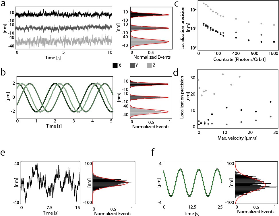
(a) The localization of a stationary particle (190 nm multifluorescent bead, Spherotech) at a countrate of >1600 photons per orbit (i.e. 320 kHz) is shown as a function of time (acquisition rate 200 Hz) for x, y and z in black, dark gray and light gray, respectively. The localization precision, determined from the standard deviation of the position of the stationary particle, was <3 nm laterally and <21 nm axially. (b) The localization precision for a moving particle (with a maximum velocity of 6.2 μm/s). An immobilized particle was moved along a sinusoidal path using a 3-axis piezo stage and the position recorded as a function of time (acquisition rate, 200 Hz) in x, y or z shown in black, dark gray and light gray respectively. A sinusoidal fit was performed (green lines) and the standard deviation of the residuals was used to determine the precision. For a count rate of >1600 photons per orbit (i.e. 320 kHz), a localization precision of <3 nm laterally and 21 nm axially was measured. (c) Count-rate dependent localization precision (average values from stationary and dynamic particles, acquisition rate 200 Hz). The values for x, y and z are shown in black, dark gray and light gray, respectively. (d) Velocity-dependent localization precision for a particle moving along the x, y and z axes. The decreased accuracy of the x axis compared to the y axis at velocities above 5 μm/s is a result of a ~ 0.1 ms delay in updating the position of the particle at the starting point of the new orbit (ϕ = 0°). (e) To measure the in vivo localization precision of the orbital tracking approach, a stationary mitochondrion inside the zebrafish was tracked at a count rate of 500 photons per orbit (i.e. 100 kHz). The trajectory data along the x axis (minor axis of the mitochondria) shows a localization precision of ~21 nm. (f) To determine the dynamic localization precision, the stationary mitochondrion was externally moved along the minor axis using a piezo stage. Similar to the dynamic precision measurement using beads, the resulting trajectory was fit using a sine wave and the standard deviation of the residuals showed a localization precision of 42 nm. The localization precision for moving mitochondria, which are usually smaller than stationary ones, was estimated from the standard deviation of the y orbit displacement, which averages 4.6 nm after removing high frequency noise by smoothing the trajectory data by five points.
-
Figure 1—figure supplement 1—source data 1
Matlab and data files for analyzing and producing graphics for particle localization from panels a-f.
- https://doi.org/10.7554/eLife.46059.004
Figure 1—figure supplement 2
Heartbeat of the larvae.
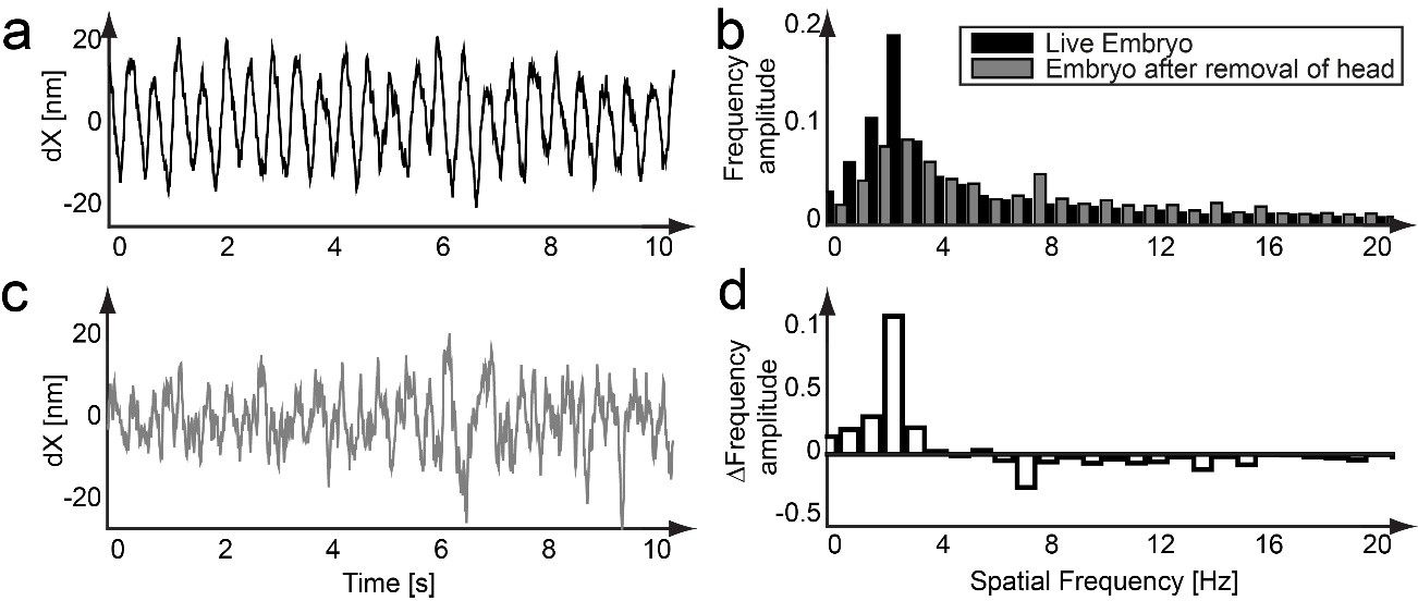
(a) Depending on the vicinity of the neuron cell to larger blood vessels, motion due to the heartbeat of the zebrafish larvae could be detected. By subtracting a smoothed trajectory (50 points = 0.5 s) from the raw data, low-frequency components (the underlying axonal structure) are filtered out and a sinusoidal signal in the y component (perpendicular to the direction of motion) of a measured trajectory becomes visible. (b) A frequency analysis of this signal revealed an underlying signal of 2.38 Hz, which corresponds to the heartbeat of a zebrafish embryo of 120–180 bpm (black bars). (c) After surgically isolating the tail of the same larvae used to acquire the trajectory from a), a second trajectory was measured. The sinusoidal signal disappeared from the trajectory b) (gray bars). (d) By subtracting the frequency spectrums from b), the heartbeat contribution to the spatial frequencies can be identified. Although motion due to the heartbeat of the zebrafish larvae can be detected, its impact on the analysis of mitochondrial transport is negligible.
-
Figure 1—figure supplement 2—source data 1
Matlab files for analyzing and producing graphics of the heartbeat analyis in panels a-d.
- https://doi.org/10.7554/eLife.46059.006
Figure 1—figure supplement 3

Influence of mitochondrial shape on localization precision.
(a) The first effect that could bias the localization precision is the size of the tracked particle. Moving mitochondria are small (~700 nm along the major axis, left) when compared to stationary ones (>1 µm along the major axis, right). The rotation of the point spread function (gray) along the orbit (black) covers a circle with a diameter of ~1 µm and entirely covers small mitochondria. However, larger mitochondria do not fall completely within the orbit of the laser, which can result in no change in fluorescence signal upon movement and thus a bias in localization upon directional changes. The second effect is the shape of the tracked particle. The intensity orbit is converted to the frequency space for further calculation and only the zero and first order Fourier coefficients are used to calculate the location of the particle. Since the shape of the particle is encoded in higher Fourier coefficients, it does not influence the localization precision. (b) To determine if the mitochondria size is influencing localization precision, individual stationary mitochondria were moved externally in a sinusoidal pattern with amplitude 2.5 µm using an xyz piezo stage. The amplitude of sinusoidal motion along the minor axis (orange triangles) could be completely recovered. Motion along the major axis (orange circles) of mitochondria longer than ~1.4 µm showed a significant reduction of the sinusoidal amplitude. For comparison, the size of the minor and major axes of moving mitochondria determined from the wide-field images are shown above the plot in black. Due to the small size of the moving mitochondria, the recorded localization data are unbiased. Mitochondria sizes were determined using the FWHM from a Gaussian fit to the intensity distribution from confocal (stationary mitochondria) and wide-field images (moving mitochondria).
-
Figure 1—figure supplement 3—source data 1
Matlab files for producing graphics of size dependent localization precision of mitochondria from panel b.
- https://doi.org/10.7554/eLife.46059.008
Figure 2 with 2 supplements
Active and stationary states of mitochondrial movement.
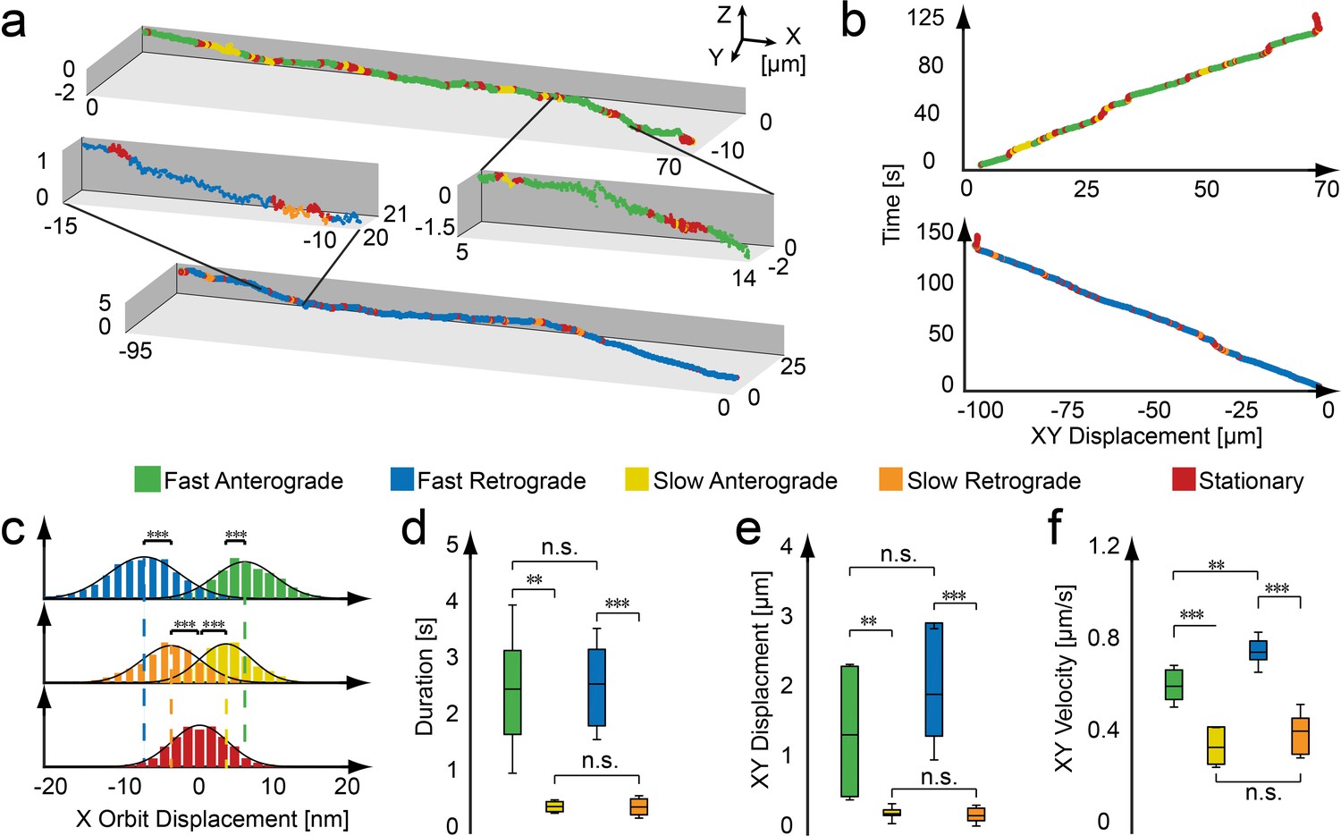
(a) Representation of an anterograde (top) and retrograde (bottom) trajectory. Color coding indicates phases of fast motion (green - anterograde; blue - retrograde), slow motion (yellow - anterograde; orange - retrograde) and stationary phases (red). (b) Kymographs of the trajectories shown in panel a. (c–f) Population properties determined from 43 mitochondrial trajectories collected from 16 embryos. (c) Orbit displacement histograms for the anterograde direction (fast: 5.8 ± 5.0 nm, n = 83,272 orbits; slow: 3.4 ± 3.7 nm, n = 27,638), the retrograde direction (fast: −7.1 ± 5.3 nm, n = 61,217; slow: −3.7 ± 4.4 nm, n = 21,984) and the stationary states (0.0 ± 3.9 nm, n = 1,153,949). Dashed lines indicate the center of the Gaussian distributions. (d) Durations of anterograde (fast: 2.5 ± 1.5 s; n = 331 states; slow 0.46 ± 0.11 s; n = 416) and retrograde motion states (fast: 2.6 ± 1.0 s; n = 220; slow 0.45 ± 0.20 s; n = 339). (e) XY displacement during anterograde (fast: 1.5 ± 1.0 µm; n = 331; slow 0.30 ± 0.15 µm; n = 416) and retrograde motion states (fast: 2.1 ± 1.0 µm; n = 220; slow 0.27 ± 0.15 µm; n = 339). (f) Lateral velocity during anterograde (fast: 0.62 ± 0.09 µm/s; n = 331; slow 0.36 ± 0.08 µm/s; n = 416) and retrograde states (fast: 0.76 ± 0.08 µm/s; n = 331; slow 0.42 ± 0.11 µm/s; n = 416). Box plot shows the average, as wells as 25 and 75 percentile; error bars indicate standard deviation. Asterisks indicate significance levels (determined by a two-sided t-test) of *: p<0.01, **: p<0.005 and ***: p<0.001. (Table 1).
-
Figure 2—source data 1
Matlab files for analyzing and producing graphics of trajectories from panel a, kymographs from panel b, and population properties from panels c-f.
- https://doi.org/10.7554/eLife.46059.017
Figure 2—figure supplement 1
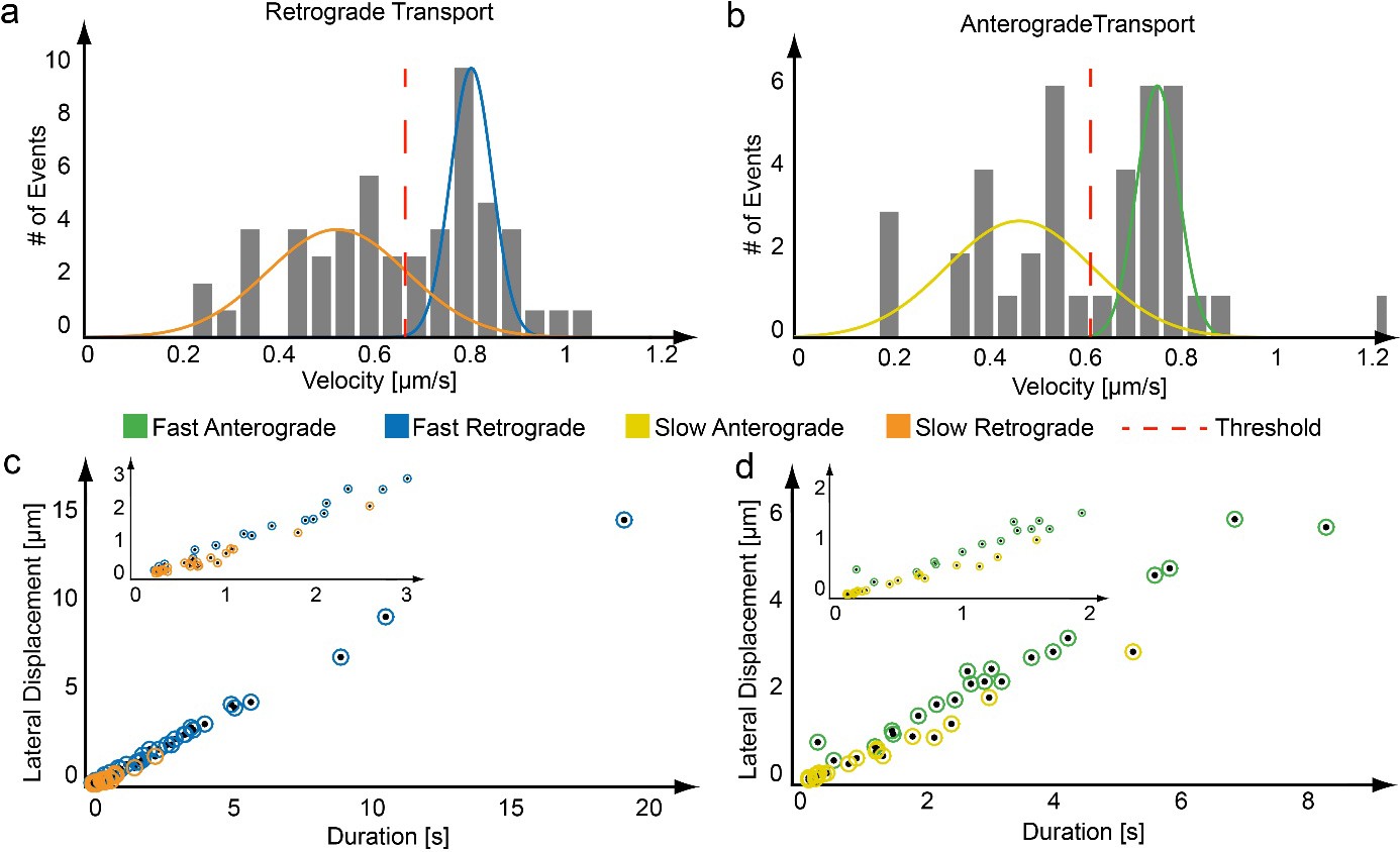
Assignment of transport populations using a maximum likelihood approach.
(a,b) From each region of active transport, an average velocity is determined. The distribution of velocities for the trajectories plotted in Figure 2 is given, which clearly shows two populations. The distribution of transport velocities from a trajectory were fit to two Gaussian functions using a maximum likelihood approach as shown for a) a retrograde and b) an anterograde moving mitochondrion. (c,d) Based on the mean velocities of the maximum likelihood fit, each active phase is assigned to either the fast or slow population (blue – fast retrograde, orange – slow retrograde, green – fast anterograde, yellow – slow anterograde).
-
Figure 2—figure supplement 1—source data 1
Matlab files for analyzing and producing graphics of velocity distribution plots from panels a and b as well as corresponding population assignment from panels c and d.
- https://doi.org/10.7554/eLife.46059.014
Figure 2—figure supplement 2
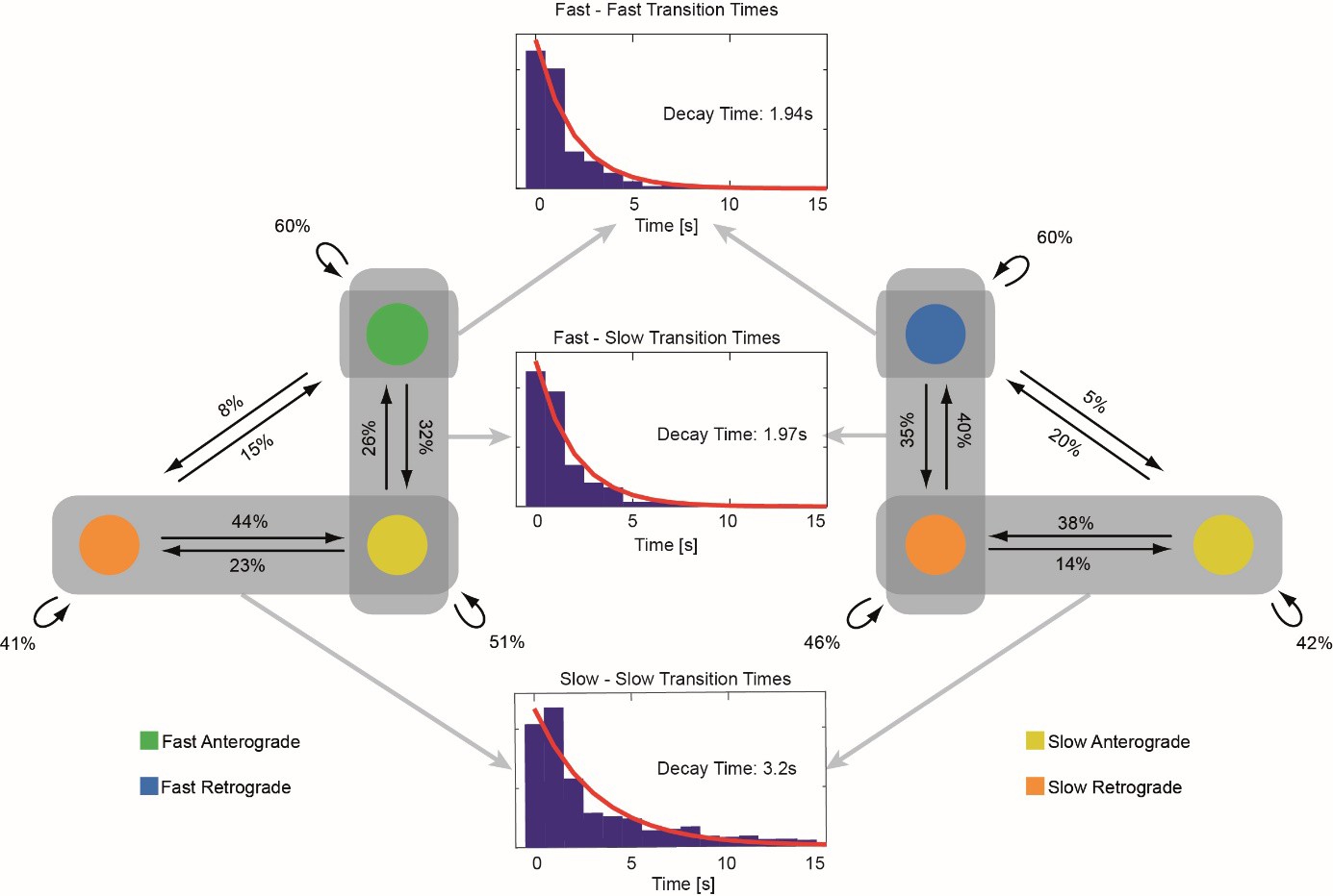
Transition pattern of mitochondria between different movement phases.
Left and right figures: A transition probability diagram is shown for retrograde and anterograde moving mitochondria respectively. The probability of transitions between different movement phases are given in the left and right diagrams (n = 1234 transitions). The distributions of pause duration (middle plots) between transitions involving the fast motion states show mono exponential decay constants of 1.94 s (fast-fast transitions) and 1.97 s (fast-slow transitions). The distribution of pause duration for transitions between slow states show a decay constant of 3.2 s. Directional transitions between the fast and slow states are rare events and no statistical relevant results could be obtained for these types of transitions.
-
Figure 2—figure supplement 2—source data 1
Matlab files for producing graphics of time decay plots.
- https://doi.org/10.7554/eLife.46059.016
Figure 3
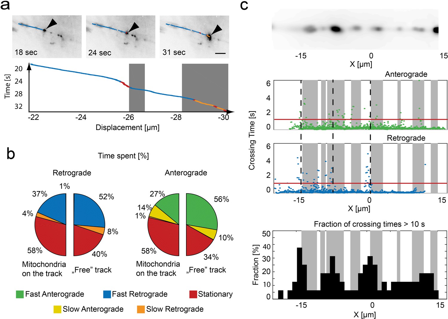
Relation of mitochondrial trajectory to local axonal environment.
(a) Mapping of the trajectory of a single mitochondrion (black arrow) onto the inverted wide-field images (scale bar, 5 µm). Bottom panel, kymograph color coded according to motion state, location of stationary mitochondria depicted in gray. (b) Pie charts indicating the fraction of time spent in each motion state related to the local presence or absence of a mitochondrion in retrograde (left) or anterograde (right) direction (n = 16 trajectories, nine fish). (c) Repetitive tracking of mitochondria over the same stretch of an axon. Upper Panel: Wide field image of the ROI showing the location of stalled mitochondria on a section of microtubules. Middle panel: The time a mitochondrion needed to transverse 100 nm is plotted as a function of position along the axon. Gray boxes indicate the presence of stationary mitochondria. The red line indicates the threshold level to identify bins of slow movement. Dashed black lines indicate locations where multiple mitochondria were observed to pause (see lower panel). Lower panel: Fraction of trajectories (plotted in 1 µm bins from mitochondria moving in both directions) along the axon showing crossing times of more than 10 s for 1 µm.
-
Figure 3—source data 1
Matlab files for analyzing and producing graphics of pie charts from panel b, crossing time of stationary mitochondria as well as fracrion of trajectories from panel c.
- https://doi.org/10.7554/eLife.46059.021
Videos
Video 1
Anterograde transport.
(Left) Wide-field video showing the anterograde transport of a photo-activated mitochondrion along a single axon. Color-coding of the trailing points indicate different movement states (green – fast anterograde, yellow – slow anterograde, orange – slow retrograde, red – stationary state; scale bar 5 µm). (Top right) Mean photon count rate of both detection channels. Downward spikes indicate long range tracking events where the tracking software is not able to track the particle for ~35–70 ms (axis dependent). The laser intensity was occasionally increased manually to ensure high tracking accuracy. (Bottom right) 3D trajectory of the moving mitochondrion. The field of view of the EMCCD camera is indicated by the gray square box, the threshold for the long-range tracking in black. Gray vertical lines indicate the position of stationary mitochondrion. After 145 s, the tracking algorithm switches to a brighter, stationary mitochondrion.
Video 2
Retrograde transport.
(Left) Wide-field video showing the retrograde transport of a photo-activated mitochondrion along a single axon. Color-coding of the trailing points indicate different movement states (blue – fast retrograde, orange – slow retrograde, yellow – slow anterograde, red – stationary state; scale bar 5 µm). (Top right) Mean photon count rate of both detection channels. Downward spikes indicate long range tracking events where the tracking software is not able to track the particle for ~35–70 ms (axis dependent).
Tables
Table 1
Dynamic states properties of untreated zebrafish embryos.
Numerical values and statistics of zebrafish embryos for data shown in Figure 2c–f. Values are gives as the average ±s.d. Significance levels were determined using a two-sided t-test). The left and right cells highlighted by the gray boxes indicate the value pair used to determine the respective p values.
| Fast anterograde | Slow anterograde | Fast retrograde | Slow retrograde | Stationary | |
|---|---|---|---|---|---|
| Duration | 2.53 ± 1.48 [s] | 0.46 ± 0.11 [s] | 2.62 ± 0.98 [s] | 0.45 ± 0.20 [s] | |
| n | 331 | 416 | 220 | 339 | |
| p | 1.7e-3 | 5.1e-5 | |||
| 0.88 | |||||
| 0.92 | |||||
| XY Displacement | 1.47 ± 0.96 [µm] | 0.30 ± 0.15 [µm] | 2.07 ± 0.97 [µm] | 0.27 ± 0.15 [µm] | |
| n | 331 | 416 | 220 | 339 | |
| p | 3.9e-3 | 2.2e-4 | |||
| 0.18 | |||||
| 0.67 | |||||
| XY Velocity | 0.62 ± 0.09 [µm/s] | 0.36 ± 0.08 [µm/s] | 0.76 ± 0.08 [µm/s] | 0.42 ± 0.11 [µm/s] | |
| n | 331 | 416 | 220 | 339 | |
| p | 2.7e-6 | 1.0e-6 | |||
| 1.6e-3 | |||||
| 0.14 | |||||
| X Orbit Displacement | 5.8 ± 5.0 [nm] | 3.4 ± 3.7 [nm] | −7.1 ± 5.3 [nm] | −3.7 ± 4.4 [nm] | 0.0 ± 3.9 [nm] |
| n | 83272 | 27638 | 61217 | 21984 | 1153949 |
| p | 2.8e-5 | 1.3e-7 | |||
| 6.1e-7 | |||||
| 5.3e-7 | |||||
| 0.49 | |||||
Table 2
Velocity comparison.
Comparison of velocities between the orbital tracking analysis and the wide-field analysis used in a previous study (Plucińska et al., 2012). The comparison between the wide-field analyses at 25°C and 28°C showed a 40% reduction in velocity, which is attributed to the reduced temperature. Due to the low time and spatial resolution, the wide-field analysis can only extract the velocity for a single population. This velocity value represents an average of the fast, slow and short stationary states, due to the inability of the wide-field analysis to reliably discriminate between these states. Values are given as the average ±s.d.
| Lateral velocity | |||
|---|---|---|---|
| Population | Tracking analysis 25°C | Wide-field recording analysis 25°C | Wide-field analysis (after Plucinska et al.) 28°C |
| Retrograde | |||
| Fast | 0.76 ± 0.08 [µm/s] | 0.55 ± 0.07 [µm/s] | 0.92 ± 0.02 [µm/s] |
| Slow | 0.42 ± 0.11 [µm/s] | ||
| Anterograde | |||
| Fast | 0.62 ± 0.09 [µm/s] | 0.45 ± 0.08 [µm/s] | 0.77 ± 0.01 [µm/s] |
| Slow | 0.36 ± 0.08 [µm/s] | ||
Key resources table
| Reagent type (species) or resource | Designation | Source or reference | Identifiers | Additional information |
|---|---|---|---|---|
| Biological sample (Danio rerio) | Roy | (Ren et al., 2002) | mpv17a9/a9 | - |
| Biological sample (Danio rerio) | Isl2b:Gal4 | (Ben Fredj et al., 2010) | Tg(−17.6isl2b:GAL4-VP16,myl7:EGFP)zc60 | - |
| Genetic reagent (UAS Constructs) | UAS:mitoTagRFP-T; UAS:mitoPAGFP; UAS:memYFP; UAS:mitoDendra2 | (Köster and Fraser, 2001) | Identified as in B - there are no specific identifiers | |
| Software | Analysis Software | this paper | https://gitlab.com/groups/3d-spt-orbital-tracking/-/shared | self-written, Matlab 2015b |
Additional files
-
Transparent reporting form
- https://doi.org/10.7554/eLife.46059.022
Download links
A two-part list of links to download the article, or parts of the article, in various formats.
Downloads (link to download the article as PDF)
Open citations (links to open the citations from this article in various online reference manager services)
Cite this article (links to download the citations from this article in formats compatible with various reference manager tools)
Nanoresolution real-time 3D orbital tracking for studying mitochondrial trafficking in vertebrate axons in vivo
eLife 8:e46059.
https://doi.org/10.7554/eLife.46059


