Figures and data in Reducing respiratory syncytial virus (RSV) hospitalization in a lower-income country by vaccinating mothers-to-be and their households

Figures
Tables
Additional files

17 figures, 6 tables and 1 additional file

Figures

Figure 1

Download asset Open asset

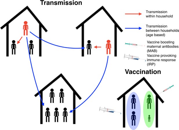
Schematic plot for the RSV transmission model and vaccination programme.

Infectious individuals (red character figures) transmit to other individuals inhabiting the same house, and to other individuals in other households based on the ages of the both the infector and infectee. Red and blue arrows represent possible realised infections over a short period of time. Bottom right household demonstrates the vaccination strategy; the mother has received a maternal antibody boosting (MAB) vaccine which increased transfer of protective antibodies to newborns (green background shading), meanwhile other household members have received an immune response provoking (IRP) vaccine (blue background shading).

Figure 2

Download asset Open asset

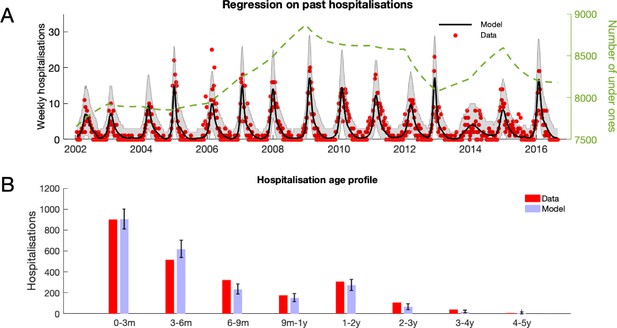
RSV hospitalisation at KCH: dynamics and age profile of hospitalised patients.

(A) Weekly RSV hospitalisations before implementation of vaccinations. Black curve gives mean prediction of RSV household transmission model after regression against weekly incidence data (red dots). Grey shaded area indicates the 99% prediction interval for the model. Also shown is the number of under ones in the population (dashed line). (B) Age profile of hospitalisations at KCH before vaccination. Error bars give 99% prediction intervals for model.

Figure 2—source data 1 Hospitalisation data, and model predictions, are given as MATLAB data files along with script for plotting figure.: https://cdn.elifesciences.org/articles/47003/elife-47003-fig2-data1-v2.zip
Download elife-47003-fig2-data1-v2.zip

Figure 3

Download asset Open asset

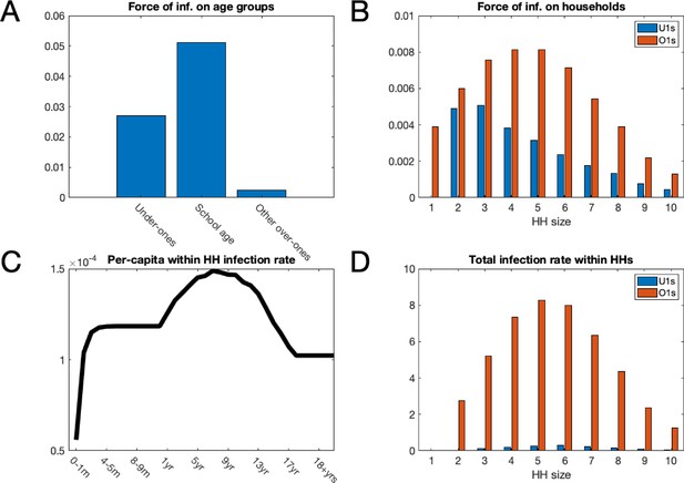
Mean force of infection (2002–2016) between households and mean infection rates within households.

(A) The mean force of infection (infectious contacts received per person per day) of RSV due to transmission from without the household on three age groups: under-ones, school age children and everyone else, including adults. (B) Mean force of infection due to transmission without the household on individuals inhabiting each household size. (C) The mean per-capita daily rate at which different age groups become infected with RSV from within their household. (D) The mean total daily rate of RSV infection within households of different sizes.

Figure 3—source data 1 The model predictions are given as MATLAB data files, along with the script for plotting figure.: https://cdn.elifesciences.org/articles/47003/elife-47003-fig3-data1-v2.zip
Download elife-47003-fig3-data1-v2.zip

Figure 4

Download asset Open asset

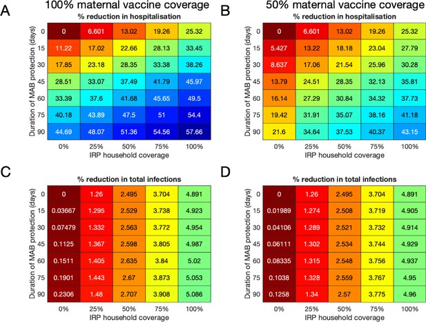
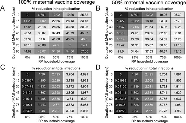
Median forecast effectiveness of RSV vaccination for different mixed strategies over a 10-year period for 100% maternal vaccine effective coverage (**A and C**) and 50% maternal vaccine effective coverage (**B and D**).

(**A and B**) Median percentage reduction in hospitalisations at KCH. (**C and D**) Percentage reduction in total RSV infections in the population.

Figure 4—source data 1 Reductions in hospitalisations and infections for each of the 500 forecasting simulations are given as MATLAB data files, along with script for plotting figure.: https://cdn.elifesciences.org/articles/47003/elife-47003-fig4-data1-v2.zip
Download elife-47003-fig4-data1-v2.zip

Figure 5

Download asset Open asset

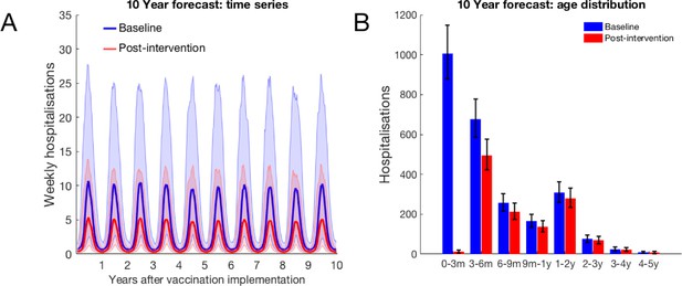
10-year forecast of RSV vaccination effectiveness for a mixed strategy of an MAB vaccine provided 75 days of additional RSV protection for newborns and a 75% IRP vaccine household coverage.

(A) Forecast weekly hospitalisations for a baseline of no vaccination (*blue*) and the mixed vaccination strategy (*red*). Shown are median forecast (*curves*) and 95% prediction intervals (*background shading*). (B) Forecast age distribution of total RSV hospitalisations at KCH. Median forecast (*bars*) and 95% prediction intervals (*error bars*).

Figure 5—source data 1 Hospitalisation predictions for each of 500 forecasting simulations is given as a MATLAB data file, along with a MATLAB function for combining the forecasting and Poisson hospitalisation rate uncertainties into a prediction interval and plotting script.: https://cdn.elifesciences.org/articles/47003/elife-47003-fig5-data1-v2.zip
Download elife-47003-fig5-data1-v2.zip

Figure 6

Download asset Open asset

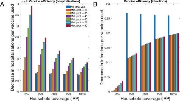
Forecast vaccination efficiency against hospitalisations and all infections, defined as number of cases averted per vaccine used (both MAB and IRP).

MAB vaccine coverage was 100% unless unavailable, however MAB protection duration varied (different coloured bars) and IRP household coverage was also varied. See Table 1 for a list of scenario. (A) Median avoided hospitalisations at KCH per vaccine over 500 simulations. (B) Median avoided RSV infections in population per vaccine over 500 simulations.

Figure 6—source data 1 A MATLAB script for converting 500 forecasting simulation outcomes into efficiency metrics, and plotting them.: https://cdn.elifesciences.org/articles/47003/elife-47003-fig6-data1-v2.zip
Download elife-47003-fig6-data1-v2.zip

Appendix 1—figure 1

Download asset Open asset

Distribution of peak month for RSV hospitalisations at KCH.

Appendix 2—figure 1

Download asset Open asset

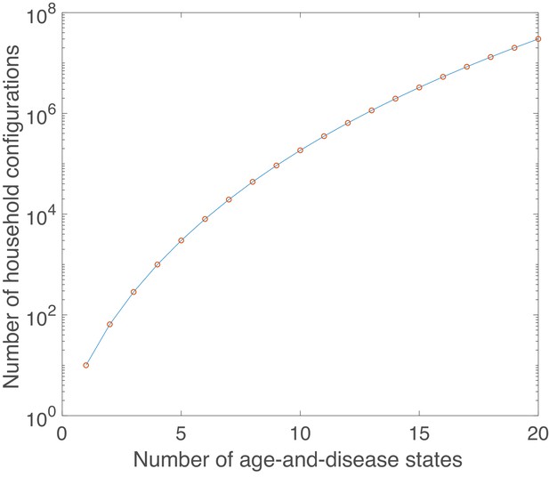
Growth in number of possible household configurations as complexity of the underlying age-and-disease state model grows.

Calculated for a maximum household size of 10.

Appendix 2—figure 2

Download asset Open asset

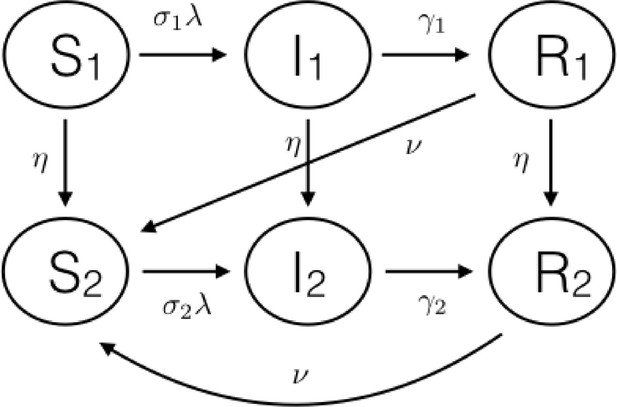
Schematic diagram of the basic age-and-disease state compartmental model for the individuals inside the households.

Appendix 2—figure 3

Download asset Open asset

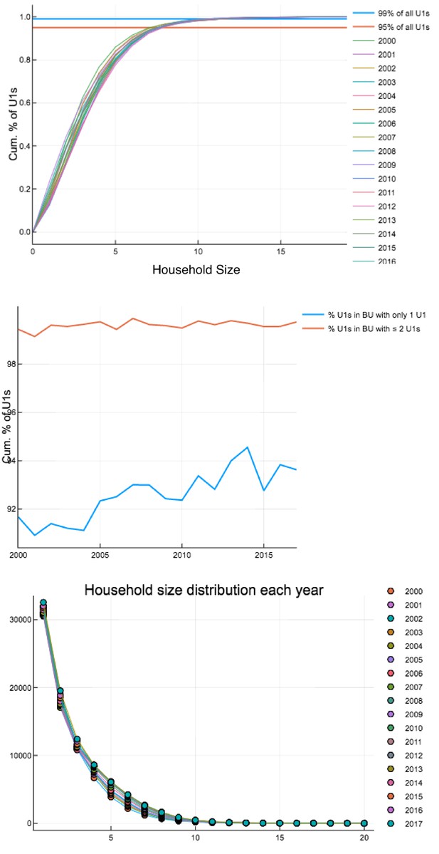
Household occupancy characteristics calculated on each 1 st Jan 2000–2017.

*Top:* Percentage of U1s in households of a certain size or smaller. *Middle:* Percentage of U1s in households with only one U1 and households with one or two U1s. *Bottom:* Household size distribution.

Appendix 2—figure 4

Download asset Open asset

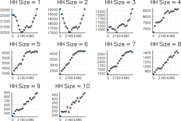
Comparison of numbers of households of sizes 1–10 on each 1 st Jan 2000–2017 (dots) against simulated values (curve).

Simulation is from Sept 2001 - Sept 2016. Horizontal axis is days since 1 st Jan 2000.

Appendix 2—figure 5

Download asset Open asset

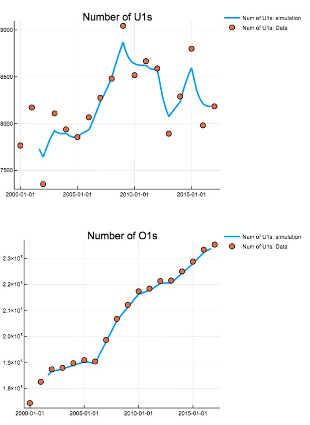
Comparison of total numbers of U1s and O1s on each 1 st Jan 2000–2017 (dots) against simulated values (curve).

Appendix 3—figure 1

Download asset Open asset

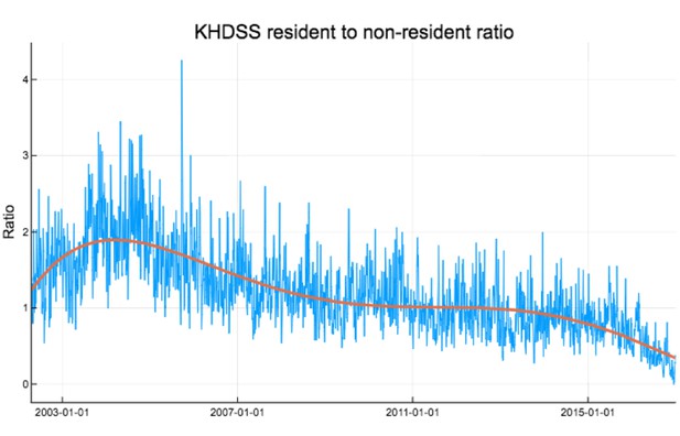
Ratio of KHDSS residents to non-residents weekly accessing KCH for confirmed RSV treatment.

Red curve is polynomial fit $R (t)$ .

Appendix 3—figure 2

Download asset Open asset

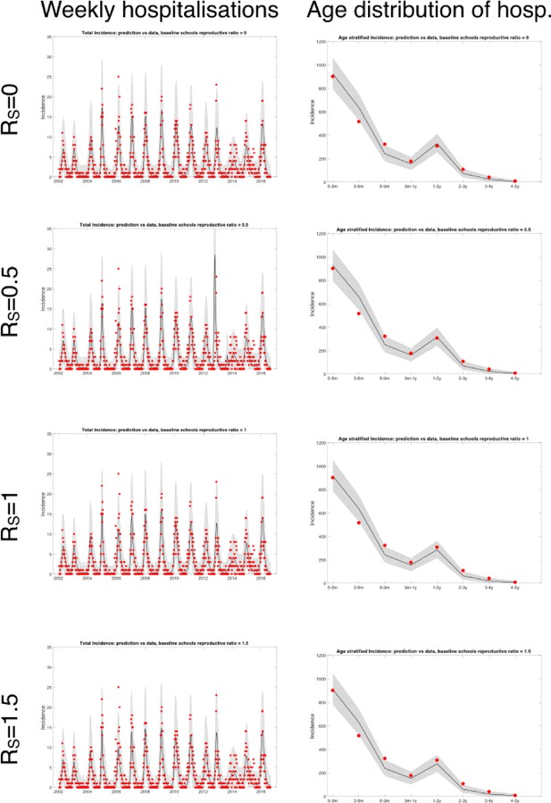
Plots of fitted weekly hospitalisations and the age distribution of hospitalisations for four scenarios (differing values of the schools based baseline $R_{S}$ ).

In each case, parameter inference was performed and the maximum likelihood estimators used.

Appendix 3—figure 3

Download asset Open asset

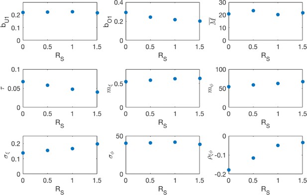
Maximum likelihood parameters for the different school transmission rate scenarios.

$b_{U 1}$ , $b_{O 1}$ are respectively the under-one and over-one mixing components of the community mixing rate matrix. $τ$ is the rate at which a household member infectiously contacts *each* other household member. $\bar{M} = 1 / α$ is the mean period of maternal protection after birth. $m = (m_{ξ} m_{ϕ})$ is the mean vector of the random seasonality, and $σ_{ξ}$ , $σ_{ϕ}$ and $ρ_{ξ ϕ}$ are respectively the standard deviations of the seasonal amplitude, seasonal phase and the correlation between the two, derived from the estimated covariance matrix $Σ_{ξ ϕ}$ .

Appendix 4—figure 1

Download asset Open asset

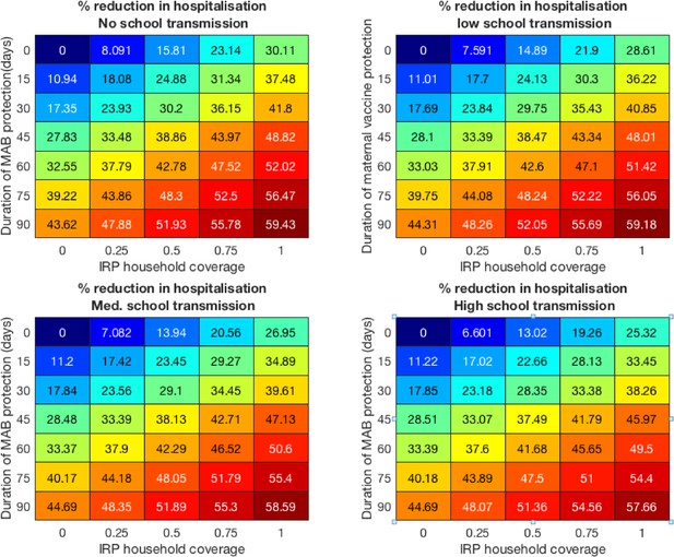
Vaccine effectiveness for the four school mixing scenarios at 100% MAB coverage.

Appendix 4—figure 2

Download asset Open asset

Colorblind-friendly version of Figure 4 from main text.

Forecast effectiveness of RSV vaccination for different mixed strategies over a 10 year period for 100% maternal vaccine effective coverage (**A and C**) and 50% maternal vaccine effective coverage (**B and D**). (**A and B**) Percentage reduction in hospitalisations at KCH. (**C and D**) Percentage reduction in total RSV infections in the population.

Tables

Table 1

Modelled vaccination scenarios.

Each combination of MAB vaccine effectiveness and coverage, with IRP vaccine coverage below was one scenario. The baseline scenario being no effective MAB vaccine and 0% coverage of IRP vaccine.

Description	Range
Additional period of protection from RSV at birth due to maternal antibody boosting (MAB) vaccine ( $P$ ).	0 (no vaccine), 15, 30, 45, 60, 75, 90 days
Coverage of mothers with MAB vaccine	50%, 100%
Coverage of households with newborns with immune response provoking (IRP) vaccination ( $V_{c o v}$ )	0%, 25%, 50%, 75%, 100%

Table 2

Parameters from literature and chosen for model.

Parameter	Description	Value	Data source
$σ_{O 1}$	Susceptibility (O1s)	0.75	Henderson et al., 1979
$ι_{2}$	relative infectiousness (O1s)	0.5	Kinyanjui et al., 2015
$ν$	Rate of waning of immunity	two per year	Agoti et al., 2012
$γ_{1}$	Rate of recovery for under-ones	1/9 per day	Hall et al., 1976
$γ_{2}$	Rate of recovery for over-ones	1/4 per day	Hall et al., 1976
$b_{S}$	Community transmission rate at schools	0,1/3,2/3,1 per day	range
$η$	Ageing rate for U1s	one per year	model choice
$ϵ$	Base external infection rate (whole population)	10 per day	model choice

Table 3

Inferred parameters.

Parameter	Description	Value
$b_{U 1}$	Community transmission rate for U1s	0.22 [0.18,0.27] per day
$b_{O 1}$	Community transmission rate for O1s	0.20 [0.18,0.21] per day
$τ$	Transmission rate to each other member of household	0.040 [0.032, 0.048] per day
$\bar{M}$	Mean duration of maternal protection at birth	21.6 [17.2, 26.1] days
$m_{ξ}$	Mean amplitude of log-seasonality	0.61 [0.51, 0.72]
$m_{ϕ}$	Mean timing of log-seasonality peak (phase)	67.7 [40.2, 77.7] days
$σ_{ξ}$	Std. amplitude of log-seasonality	0.20 [0.098,0.31]
$σ_{ϕ}$	Std. timing of log-seasonality peak (phase)	38.7 [30.0, 48.5] days
$ρ_{ξ ϕ}$	Corr. coefficient between log-seasonal amplitude and phase	−0.035 [-0.12, 0.072]

Appendix 3—table 1

Parameters estimated from KHDSS data.

Parameter	Description	Value	Data source
μ(n, t)	Birth/turnover rate for households of size n on day t	Varies, see above	KHDSS
r(n, t)	Rate of change of numbers of households of size n on day t	Varies, see above	KHDSS
P_H→A,t	Conditional age distribution given household config. on day t	Varies, see above	KHDSS
P_A→H,t	Conditional household config. distribution given age category on day t	Varies, see above	KHDSS

Appendix 3—table 2

Age-dependent hospitalisation probabilities per infection derived from Kinyanjui et al., 2015.

Age category	Probability of hospitalisation per infection
0-1 month	0.10
1-2 month	0.10
2-3 month	0.063
3-4 month	0.059
4-5 month	0.054
5-6 month	0.025
6-7 month	0.019
7-8 month	0.022
8-9 month	0.012
9-10 month	0.016
10-11 month	0.013
11-12 month	5.1x10⁻³
1-2 years old	2.6x10⁻³
2-3 years old	7.5x10⁻⁴
3-4 years old	2.2x10⁻⁴
4-5 years old	3.8x10⁻⁵

Appendix 3—table 3

Model parameters inferred from hospitalisation data.

b_U1	Community transmission rate for U1s	0.22 [0.18,0.27] per day
b_O1	Community transmission rate for O1s	0.20 [0.18,0.21] per day
τ	Transmission rate to each other member of household	0.040 [0.032, 0.048] per day
M	Mean duration of maternal protec- tion at birth	21.6 [17.2, 26.1] days
m_ξ	Mean amplitude of log-seasonality	0.61 [0.51, 0.72]
m_φ	Mean timing of log-seasonality peak (phase)	67.7 [40.2, 77.7] days
σ_ξ	Std. amplitude of log-seasonality	0.20 [0.098,0.31]
σ_φ	Std. timing of log-seasonality peak (phase)	38.7 [30.0, 48.5] days
ρ_ξφ	Corr. coefficient between log- seasonal amplitude and phase	-0.035 [-0.12, 0.072]

Additional files

Transparent reporting form: https://cdn.elifesciences.org/articles/47003/elife-47003-transrepform-v2.docx
Download elife-47003-transrepform-v2.docx

Download links

A two-part list of links to download the article, or parts of the article, in various formats.

Downloads (link to download the article as PDF)

Article PDF

Open citations (links to open the citations from this article in various online reference manager services)

Mendeley

Cite this article (links to download the citations from this article in formats compatible with various reference manager tools)

Samuel PC Brand
Patrick Munywoki
David Walumbe
Matthew J Keeling
David James Nokes

(2020)

Reducing respiratory syncytial virus (RSV) hospitalization in a lower-income country by vaccinating mothers-to-be and their households

eLife 9:e47003.

https://doi.org/10.7554/eLife.47003

Figures

Schematic plot for the RSV transmission model and vaccination programme.

RSV hospitalisation at KCH: dynamics and age profile of hospitalised patients.

Figure 2—source data 1

Mean force of infection (2002–2016) between households and mean infection rates within households.

Figure 3—source data 1

Median forecast effectiveness of RSV vaccination for different mixed strategies over a 10-year period for 100% maternal vaccine effective coverage (A and C) and 50% maternal vaccine effective coverage (B and D).

Figure 4—source data 1

10-year forecast of RSV vaccination effectiveness for a mixed strategy of an MAB vaccine provided 75 days of additional RSV protection for newborns and a 75% IRP vaccine household coverage.

Figure 5—source data 1

Forecast vaccination efficiency against hospitalisations and all infections, defined as number of cases averted per vaccine used (both MAB and IRP).

Figure 6—source data 1

Distribution of peak month for RSV hospitalisations at KCH.

Growth in number of possible household configurations as complexity of the underlying age-and-disease state model grows.

Schematic diagram of the basic age-and-disease state compartmental model for the individuals inside the households.

Household occupancy characteristics calculated on each 1 st Jan 2000–2017.

Comparison of numbers of households of sizes 1–10 on each 1 st Jan 2000–2017 (dots) against simulated values (curve).

Comparison of total numbers of U1s and O1s on each 1 st Jan 2000–2017 (dots) against simulated values (curve).

Ratio of KHDSS residents to non-residents weekly accessing KCH for confirmed RSV treatment.

Plots of fitted weekly hospitalisations and the age distribution of hospitalisations for four scenarios (differing values of the schools based baseline $R_{S}$ ).

Maximum likelihood parameters for the different school transmission rate scenarios.

Vaccine effectiveness for the four school mixing scenarios at 100% MAB coverage.

Colorblind-friendly version of Figure 4 from main text.

Tables

Modelled vaccination scenarios.

Parameters from literature and chosen for model.

Inferred parameters.

Parameters estimated from KHDSS data.

Age-dependent hospitalisation probabilities per infection derived from Kinyanjui et al., 2015.

Model parameters inferred from hospitalisation data.

Additional files

Transparent reporting form

Download links

Downloads (link to download the article as PDF)

Open citations (links to open the citations from this article in various online reference manager services)

Cite this article (links to download the citations from this article in formats compatible with various reference manager tools)

Be the first to read new articles from eLife

Share this article

Cite this article

Schematic plot for the RSV transmission model and vaccination programme.

RSV hospitalisation at KCH: dynamics and age profile of hospitalised patients.

Figure 2—source data 1

Mean force of infection (2002–2016) between households and mean infection rates within households.

Figure 3—source data 1

Median forecast effectiveness of RSV vaccination for different mixed strategies over a 10-year period for 100% maternal vaccine effective coverage (A and C) and 50% maternal vaccine effective coverage (B and D).

Figure 4—source data 1

10-year forecast of RSV vaccination effectiveness for a mixed strategy of an MAB vaccine provided 75 days of additional RSV protection for newborns and a 75% IRP vaccine household coverage.

Figure 5—source data 1

Forecast vaccination efficiency against hospitalisations and all infections, defined as number of cases averted per vaccine used (both MAB and IRP).

Figure 6—source data 1

Distribution of peak month for RSV hospitalisations at KCH.

Growth in number of possible household configurations as complexity of the underlying age-and-disease state model grows.

Schematic diagram of the basic age-and-disease state compartmental model for the individuals inside the households.

Household occupancy characteristics calculated on each 1 st Jan 2000–2017.

Comparison of numbers of households of sizes 1–10 on each 1 st Jan 2000–2017 (dots) against simulated values (curve).

Comparison of total numbers of U1s and O1s on each 1 st Jan 2000–2017 (dots) against simulated values (curve).

Ratio of KHDSS residents to non-residents weekly accessing KCH for confirmed RSV treatment.

Plots of fitted weekly hospitalisations and the age distribution of hospitalisations for four scenarios (differing values of the schools based baseline RS).

Maximum likelihood parameters for the different school transmission rate scenarios.

Vaccine effectiveness for the four school mixing scenarios at 100% MAB coverage.

Colorblind-friendly version of Figure 4 from main text.

Modelled vaccination scenarios.

Parameters from literature and chosen for model.

Inferred parameters.

Parameters estimated from KHDSS data.

Age-dependent hospitalisation probabilities per infection derived from Kinyanjui et al., 2015.

Model parameters inferred from hospitalisation data.

Transparent reporting form

Downloads (link to download the article as PDF)

Open citations (links to open the citations from this article in various online reference manager services)

Cite this article (links to download the citations from this article in formats compatible with various reference manager tools)

Plots of fitted weekly hospitalisations and the age distribution of hospitalisations for four scenarios (differing values of the schools based baseline $R_{S}$ ).