Variability in locomotor dynamics reveals the critical role of feedback in task control
- Department of Electrical and Electronics Engineering, Hacettepe University, Turkey
- Laboratory of Computational Sensing and Robotics, Johns Hopkins University, United States
- Department of Biological Sciences, New Jersey Institute of Technology, United States
- Department of Mechanical Engineering, Johns Hopkins University, United States
- Department of Electrical and Electronics Engineering, Middle East Technical University, Turkey
Figures
Figure 1 with 4 supplements

Experimental analysis of refuge tracking behavior.
(A) Eigenmannia virescens maintains its position, , in a moving refuge. is the position of the moving refuge. (B) A feedback control system model for refuge tracking. The feedback controller maps the error signal, , to a control signal, . The plant , in turn, generates fore-aft movements . We used measurements of the nodal point as to estimate in each fish, which was subsequently used to infer . (C) Eigenmannia virescens partitions its ribbon fin into two counter-propagating waves that generate opposing forces (Sefati et al., 2013; Ruiz-Torres et al., 2013). The rostral-to-caudal and caudal-to-rostral waves collide at the nodal point (green line). Movements of the nodal point serve as a proxy for the control signal, . Gray lines indicate the positions of the peaks and troughs of the traveling waves over time. In this trial, the refuge was following a sinusoidal trajectory at 2.05 Hz. (D) Movement of the nodal point , position of the fish , and position of the refuge of 13 trials at 0.95 Hz. Semi-transparent lines represent data from individual trials, green and blue lines are the means.
Figure 1—figure supplement 1
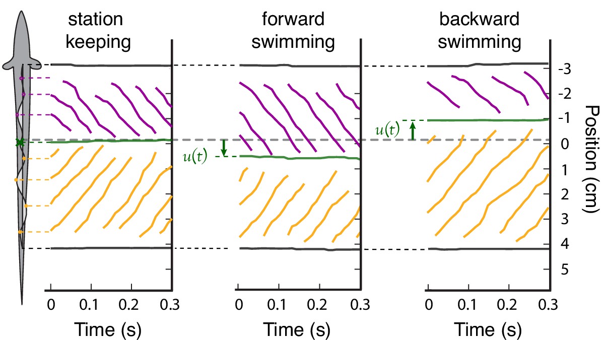
Steady-state position of the nodal point.
Three examples of steady-state, constant-speed swimming that illustrate how the peaks and troughs of the ribbon fin wave propagate toward the nodal point. The purple lines indicate the positions of the peaks and troughs of the traveling waves initiated at the rostral end of the ribbon fin. Orange lines indicate the traveling waves initiated at the caudal end of the ribbon fin. These waves meet at the nodal point (green). (left) Peaks, troughs, and nodal point reference location during station keeping, . (center) The nodal point shifts caudally relative to the reference position during steady-state forward swimming, and (right) shifts rostrally for backward swimming, .
Figure 1—figure supplement 2
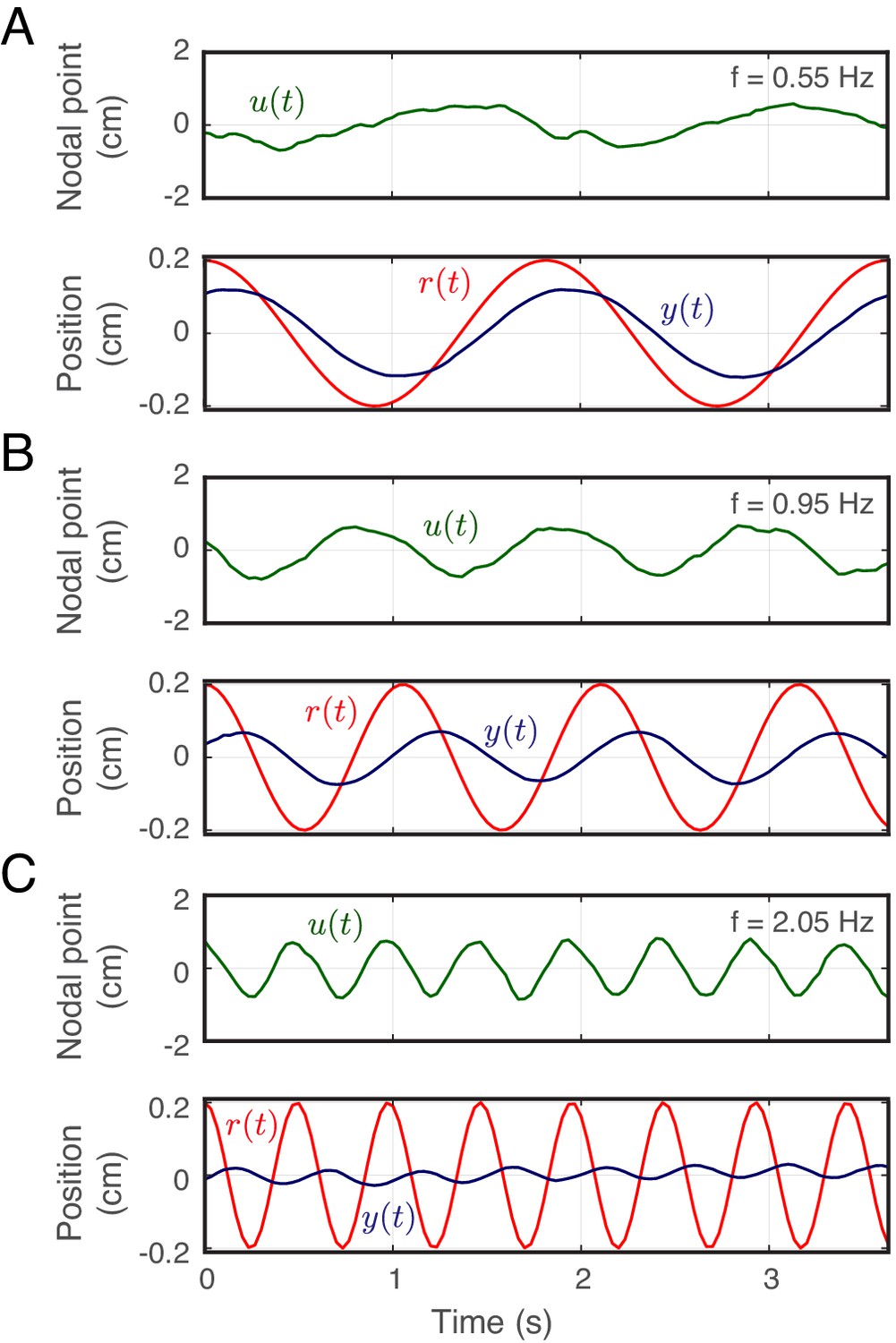
Movement of the refuge, fish and nodal point.
Averaged movements (across all trials for one fish) of the nodal point (green) and the fish (blue) with respect to refuge movements (red) at (A) 0.55 Hz, (B) 0.95 Hz, and (C) 2.05 Hz.
Figure 1—video 1
A real-time video recorded at 30 fps from below of an Eigenmannia virescens tracking a moving refuge at 0.55 Hz.
The movement of the refuge and fish are plotted below the video.
Figure 1—video 2
A high-speed video recorded at 100 fps from below an Eigenmannia virescens while tracking a moving refuge at 2.05 Hz.
The video is stabilized with respect to fish position to illustrate the movements of the head and tail waves that form the nodal point. The inset shows the rectangular area around the ribbon fin of the fish. The video is played in real-time (10 repetitions), at 0.3 × speed (3 repetitions) and at 0.1 × speed (1 repetition).
Figure 2
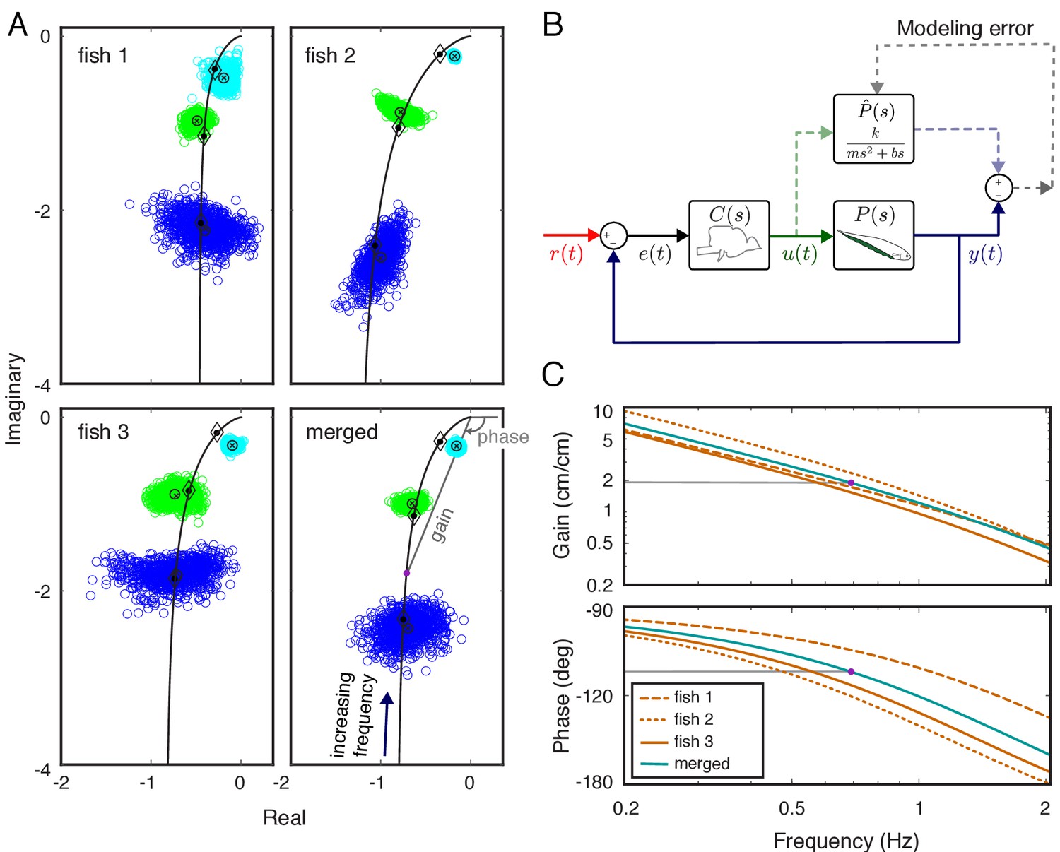
System identification of plant dynamics.
(A) Nyquist plots of the estimated plant models for each individual fish and the merged fish. Blue, green and cyan point clouds correspond to bootstrapped data estimates for the low (0.55 Hz), medium (0.95 Hz) and high (2.05 Hz) frequencies, respectively. Black circles and cross marks represent the mean for measured and bootstrapped data, respectively. Black lines represent the response of the estimated model with diamonds indicating their values at the test frequencies. Each point on the black lines correspond to the complex-valued frequency response of the plant model at a specific frequency. For example, the purple dot on the lower-right panel corresponds to the merged-plant-model’s response at 0.7 Hz. The gain and phase associated with this response are shown on the associated Bode plots given in (C). (B) Reconciliation of physics-based and data-driven models. The solid lines represent the natural feedback control system used by the fish for refuge tracking. The dashed lines represent copies of signals used for parametric system identification. represents the parametric transfer function for the plant dynamics of the fish with ‘unknown’ system parameters. The parametric system identification estimates these parameters via minimizing the difference (modeling error) between the actual output of the fish and the prediction of the model. (C) Gain and phase plots of the frequency response functions of the estimated parametric models for each fish and the merged fish corresponding to the black lines in (A).
Figure 3
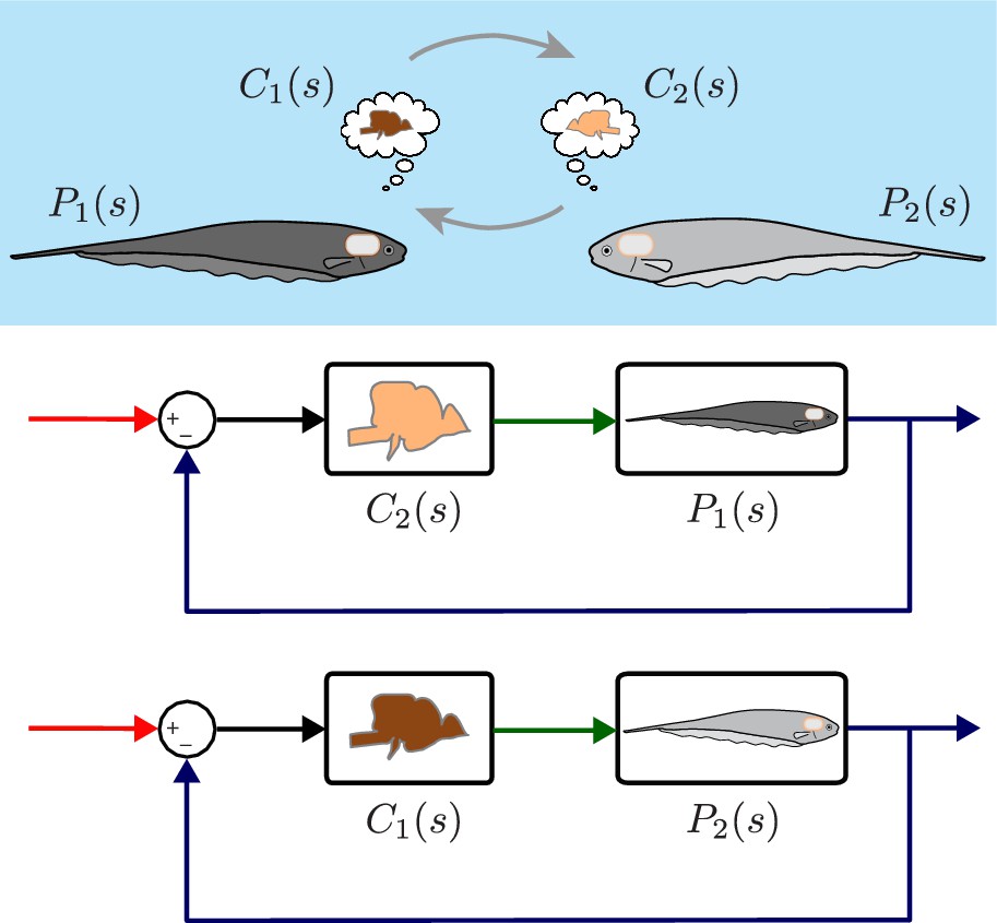
Computational brain swapping between fish.
We computationally swapped the individually tailored controllers between fish. The feedback control diagrams illustrate computational brain swaps. The controller from the light gray fish, , is used to control the plant of the dark gray fish, , and vice versa.
Figure 4
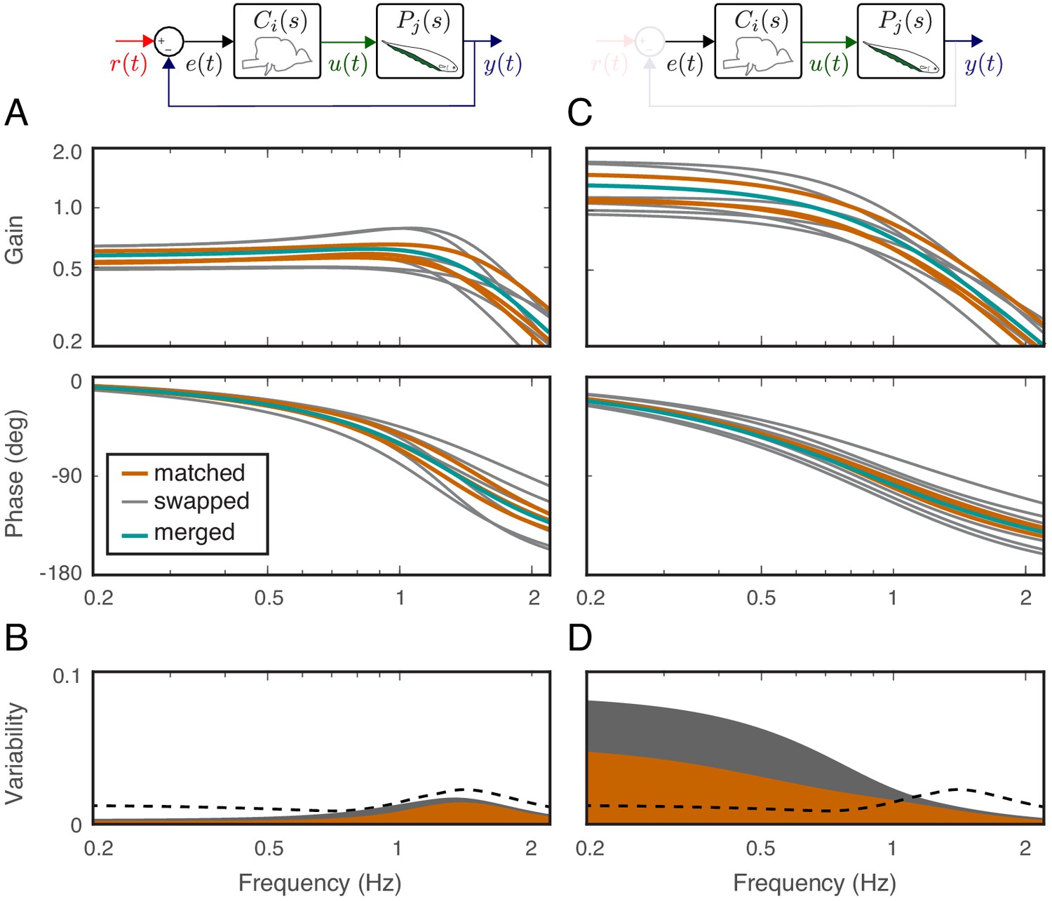
Effects of feedback on behavioral variability.
At the top of each column is a control diagram that corresponds to all figures in that column. (A) Frequency-response gain and phase plots of the estimated input–output models for the matched (orange), swapped (gray), and merged (green) fish in a feedback control topology. (B) Variability of the matched (orange) and swapped (gray) models. Dashed line is the behavioral variability observed in the tracking data across fish. (C) Same as in (B) but for the loop gain, . (D) Same as in (C) but for the loop gain, .
Figure 5
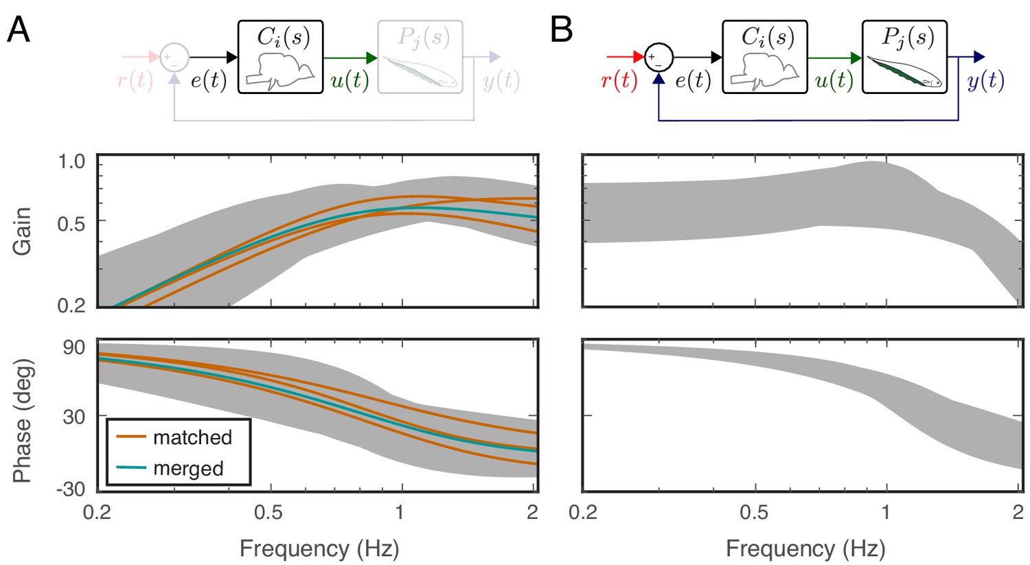
Feedback controllers satisfying the behavioral variability.
(A) Bode plots for the estimated controllers for the matched (orange) and merged (green) fish under feedback control. Each controller exhibits high-pass filter behavior across the frequency range of interest. Gray shaded regions represent the range of controllers that produce behavioral responses consistent with behavioral variability. (B) The range of behavioral input–output transfer functions consistent with behavioral variability.
Tables
Table 1
Estimated parameters of the plant model for each fish as well as the merged fish.
| Fish 1 | Fish 2 | Fish 3 | Merged | |
|---|---|---|---|---|
| 0.3228 | 0.2200 | 0.1622 | 0.2385 | |
| 0.0417 | 0.0186 | 0.0218 | 0.0269 | |
| 0.0025 | 0.0025 | 0.0025 | 0.0025 |
Table 2
Estimated parameters of the second order input-output model for each fish as well as the merged fish.
| Fish 1 | Fish 2 | Fish 3 | Merged | |
|---|---|---|---|---|
| 0.53 | 0.60 | 0.52 | 0.57 | |
| 0.58 | 0.55 | 0.52 | 0.55 | |
| 8.55 | 9.51 | 7.88 | 8.50 |
Additional files
Download links
A two-part list of links to download the article, or parts of the article, in various formats.
Downloads (link to download the article as PDF)
Open citations (links to open the citations from this article in various online reference manager services)
Cite this article (links to download the citations from this article in formats compatible with various reference manager tools)
Variability in locomotor dynamics reveals the critical role of feedback in task control
eLife 9:e51219.
https://doi.org/10.7554/eLife.51219


