Inter- and intra-animal variation in the integrative properties of stellate cells in the medial entorhinal cortex
- Centre for Discovery Brain Sciences, University of Edinburgh, United Kingdom
- The Alan Turing Institute, United States
- School of Mathematics, Maxwell Institute and Centre for Statistics, University of Edinburgh, United Kingdom
Figures
Figure 1 with 5 supplements
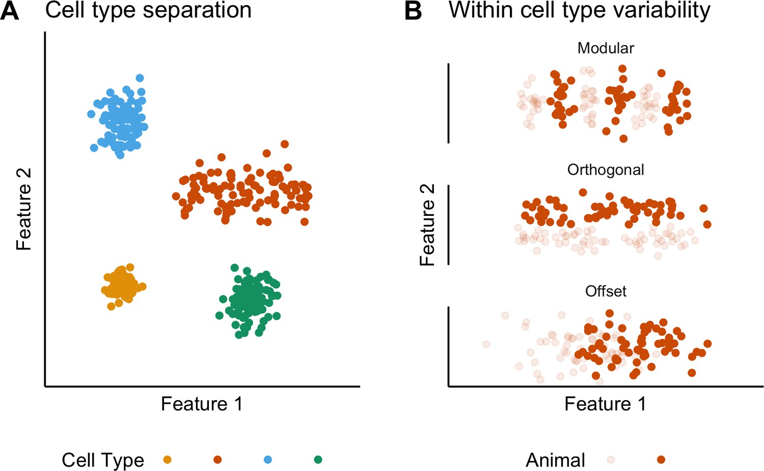
Classification and variability of neuronal cell types.
(A) Neuronal cell types are identifiable by features clustering around a distinct point (blue, green and yellow) or a line (orange) in feature space. The clustering implies that neuron types are defined by either a single set point (blue, green and yellow) or by multiple set points spread along a line (orange). (B) Phenotypic variability of a single neuron type could result from distinct set points that subdivide the neuron type but appear continuous when data from multiple animals are combined (modular), from differences in components of a set point that do not extend along a continuum but that in different animals cluster at different locations in feature space (orthogonal), or from differences between animals in the range covered by a continuum of set points (offset). These distinct forms of variability can only be made apparent by measuring the features of many neurons from multiple animals.
Figure 1—figure supplement 1
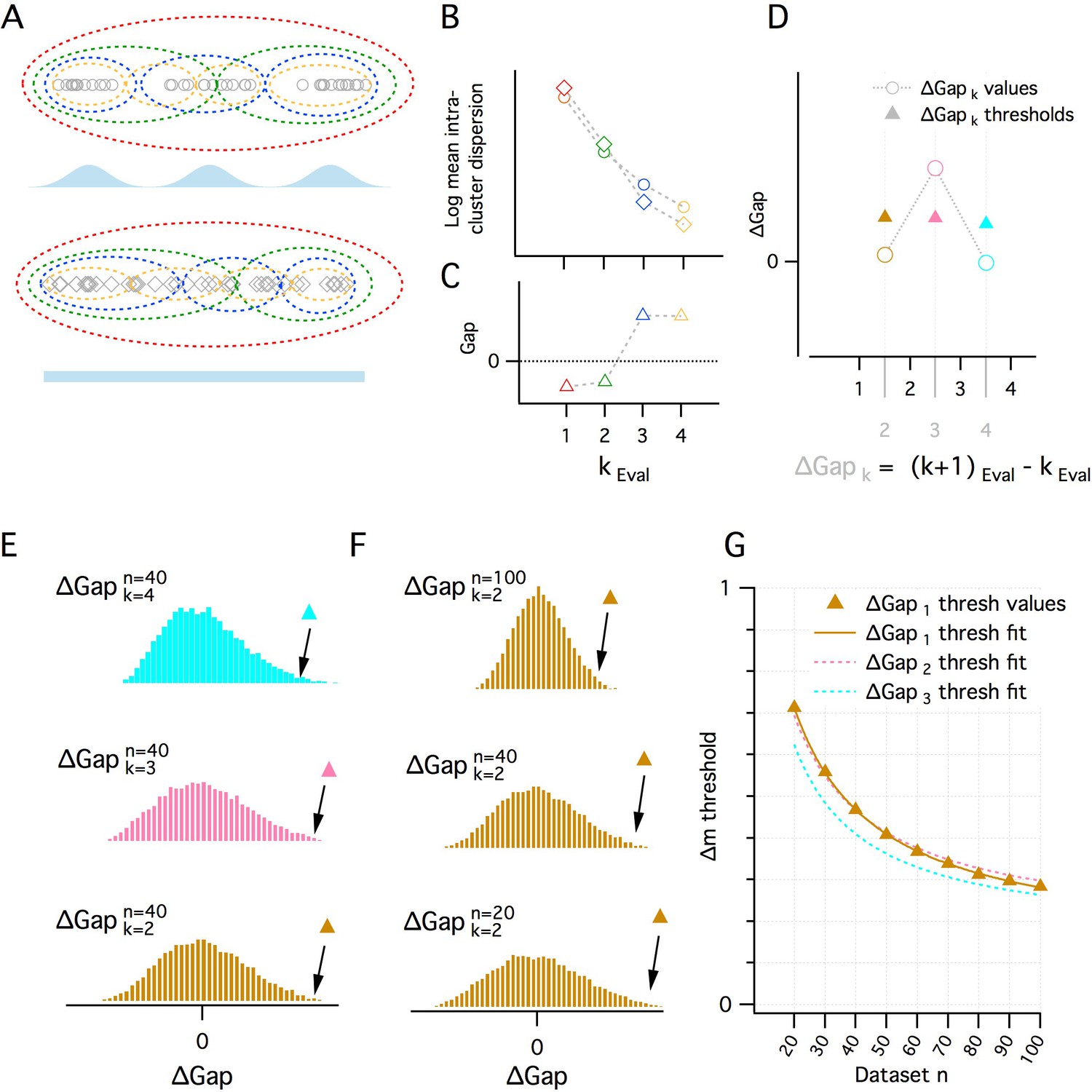
A quantitative adaptation of the gap statistic clustering algorithm.
(A–C) Logic of the gap statistic. (A) Simulated clustered dataset with three modes (k = 3) (open gray circles) (upper) and the corresponding simulated reference dataset drawn from a uniform distribution with lower and upper limits set by the minimum and maximum values from the corresponding clustered dataset (open gray diamonds). Data were allocated to clusters by running a K-means algorithm 20 times on each set of data and selecting the partition with the lowest average intracluster dispersion. Red, green, blue and yellow dashed ovals show a realization of the data subsets allocated to each cluster when kEval = 1, 2, 3 and 4 modes. (B) The average value of the log intracluster dispersion for the clustered (open circles) and reference (open diamonds) datasets for each value of k tested in panel (A). (C) Gap values resulting from the difference between the clustered and reference values for each k in panel (B). Many (≥500 in this paper) reference distributions are generated and their mean intracluster dispersion values are subtracted from those arising from the clustered distribution to maximize the reliability of the Gap values. (D) A procedure for selecting the optimal k depending on the associated gap values. Quantitative procedure for selecting optimal k (kest). ∆Gap values (open circles) are obtained by subtracting from the Gap value of a given k the Gap value for the previous k (∆Gapk = Gapk – Gapk-1). For each ∆Gapk, if the ∆Gap value is greater than a threshold (filled triangles) associated with that ∆Gapk, that ∆Gapk will be kest, if no ∆Gap exceeds, the threshold, kest = 1. In the figure, for ∆Gapk = 2, 3, 4 (brown, pink and cyan), the ∆Gap value exceeds its threshold only when ∆Gapk = 3. Therefore kest = 3. (E–G) Determination of ∆Gapk thresholds. (E) Histograms of ∆Gap values calculated from 20,000 simulated datasets drawn from uniform distributions for each ∆Gapk (brown, pink and cyan, respectively, for ∆Gapk = 2, 3, 4) for a single dataset size (n = 40). ∆Gap thresholds (filled triangles) are the values beyond which 1% of the ∆Gap values fall and vary with ∆Gapk. (F) Histograms of ∆Gap values for a range of dataset sizes (n = 20, 40, 100) and their associated thresholds. (G) Plot of the ∆Gap thresholds as a function of dataset size and ∆Gapk. For separate ∆Gapk, ∆Gap threshold values are fitted well by a hyperbolic function of dataset size. These fits provide a practical method of finding the appropriate ∆Gap threshold for an arbitrary dataset size.
Figure 1—figure supplement 2

Discrimination of continuous from modular organizations using the adapted gap statistic algorithm.
(A) Simulated datasets (each n = 40) drawn from continuous (uniform, k = 1 mode) (upper) and modular (multimodal mixture of Gaussians with k = 2 modes) (lower) distributions, and plotted against simulated dorsoventral locations. Also shown are the probability density functions (pdf) used to generate each dataset (light blue) and the densities estimated post-hoc from the generated data as kernel smoothed densities (light gray pdfs). (B) Histograms showing the distribution of kest from 1000 simulated datasets drawn from each pdf in panel (A). kest is determined for each dataset by a modified gap statistic algorithm (see Figure 1—figure supplement 1 above). When kest = 1, the dataset is considered to be continuous (unclustered), when kest ≥2, the dataset is considered to be modular (clustered). The algorithm operates only on the feature values and does not use location information. (C) Illustration of a set of clustered (k = 2) pdfs with the distance (in standard deviations) between clusters ranging from 2 to 6 (upper). Systematic evaluation of the ability of the modified gap statistic algorithm to detect clustered organization (kest ≥2) in simulated datasets of different size (n = 20 to 100) drawn from the clustered (filled blue) and continuous (open blue) pdfs (lower). The proportion of datasets drawn from the continuous distribution that have kest ≥2 is the false positive (FP) rate (pFP = ~0.07). The light gray filled circle shows the smallest dataset size (n = 40) with SD = 5, where the proportion of datasets detected as clustered (pdetect) is ~0.8. (D). Plot showing how pdetect at n = 40, SD = 5 changes when datasets are drawn from pdfs with different numbers of clusters (n modes from 2 to 8). Further evaluation of the analysis of additional clusters is represented in the following figure.
Figure 1—figure supplement 3
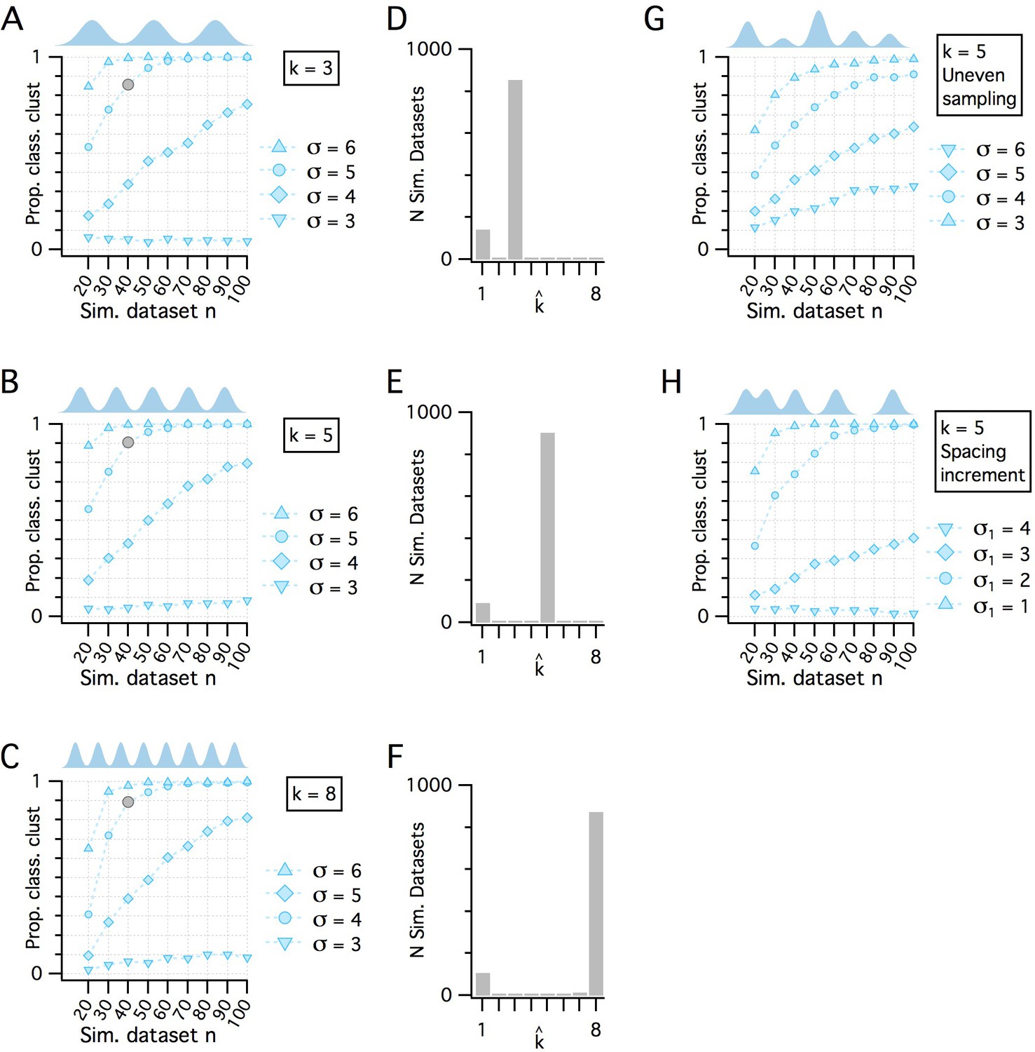
Additional evaluation of the adapted gap statistic algorithm.
(A–C) Plots showing how pdetect (the ability of the modified gap statistic algorithm to detect clustered organization) depends on dataset size and separation between cluster modes in simulated datasets drawn from clustered pdfs with different numbers of modes. The gray markers indicate n = 40, SD = 5 (as shown in Figure 1E). In each plot, pdetect is shown as a function of simulated dataset size and separation between modes when k = 3 (A), k = 5 (B) and k = 8 (C), which was the maximum number of clusters evaluated. (D–F) Histograms showing the counts of kest from the 1000 simulated n = 40, SD = 5 datasets (gray filled circles) illustrated in panels (A–C), respectively. (G) pdetect as a function of dataset size and mode separation with k = 5 when cluster modes are unevenly sampled. Sample sizes from clusters vary randomly with each dataset. A single mode can contribute from all to none of the points in any simulated dataset. (H) pdetect as a function of dataset size and mode separation with k = 5 when the distance between mode centers increases by a factor of sqrt(2) between sequential cluster pairs. Data are shown for different initial separations (the distance between the first two cluster centers) ranging from 1 to 4 (with corresponding separations between the final cluster pair ranging from 4 to 16).
Figure 1—figure supplement 4
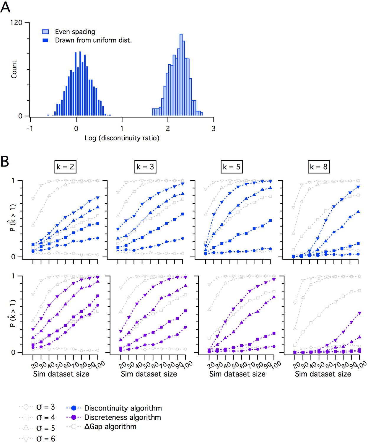
Comparing the adapted gap statistic algorithm with discontinuity measures for discreteness.
(A) Counts of log discontinuity ratio scores generated from a simulated uniform data distribution. The data distribution was ordered and then sampled either at positions drawn at random from a uniform distribution (dark blue) or at positions with a fixed increment (light blue). For the data sampled at random positions, approximately half of the scores are >0 and for even sampling all scores are >0. Therefore, a threshold score >0 does not distinguish discrete from continuous distributions. (B) Comparison of pdetect as a function of dataset size for the adapted gap statistic algorithm, the discontinuity (upper) and the discreteness algorithm (lower). Each algorithm is adjusted to yield a 7% false positive rate. Each column shows simulations of data with different numbers of modes (k).
Figure 1—figure supplement 5

Evaluation of modularity of grid firing using an adapted gap statistic algorithm.
Examples of grid spacing for individual neurons (crosses) from different mice. Kernel smoothed densities (KSDs) were generated with either a wide (solid gray) or a narrow (dashed lines) kernel. The number of modes estimated using the modified gap statistic algorithm is ≥ 2 for all but one animal (animal 4) with n ≥ 20 (animals 3 and 7 have < 20 recorded cells). We did not have location information for animal 2.
Figure 2 with 1 supplement
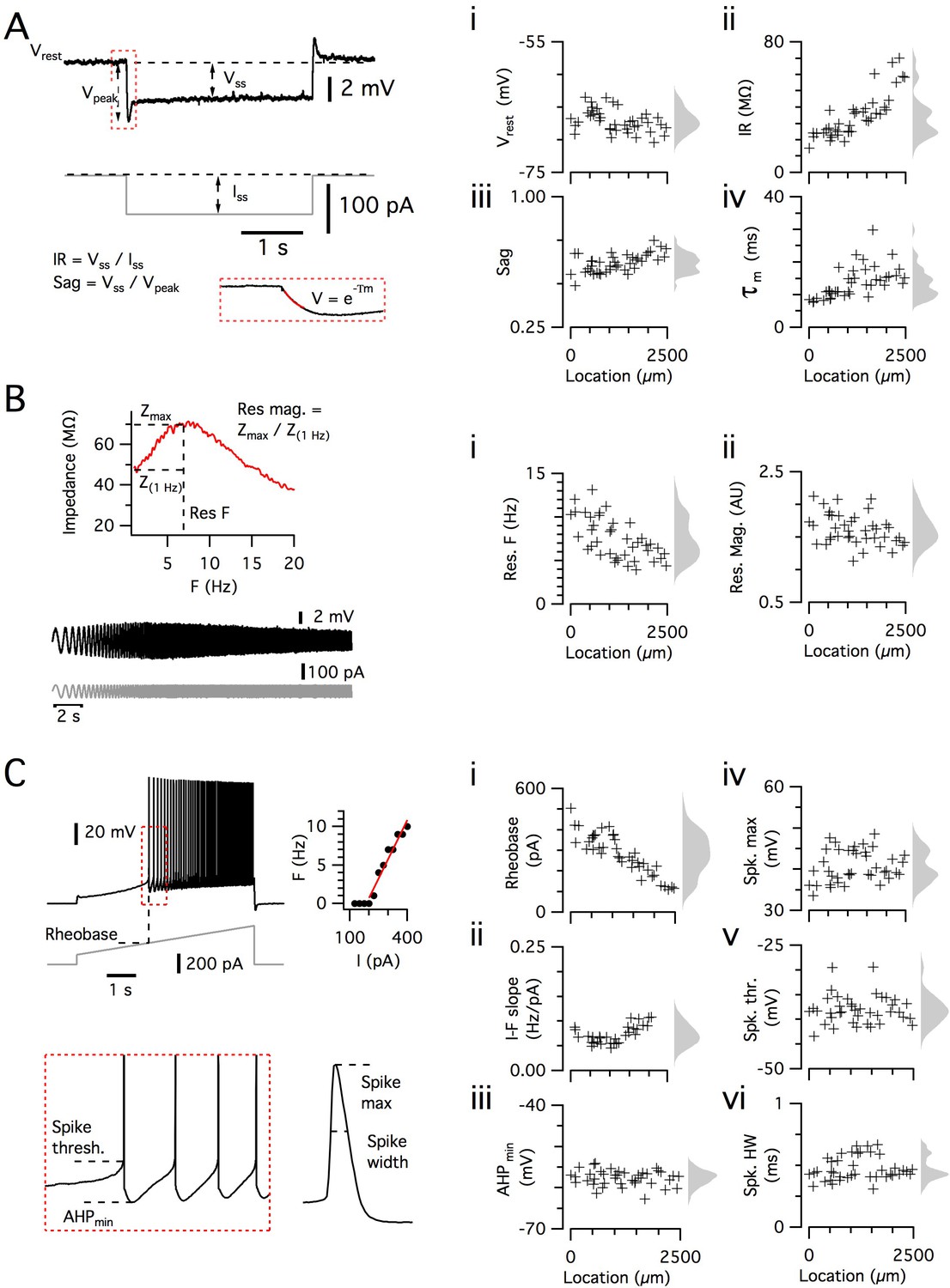
Dorsoventral organization of intrinsic properties of stellate cells from a single animal.
(A–C) Waveforms (gray traces) and example responses (black traces) from a single mouse for step (A), ZAP (B) and ramp (C) stimuli (left). The properties derived from each protocol are shown plotted against recording location (each data point is a black cross) (right). KSDs with arbitrary bandwidth are displayed to the right of each data plot to facilitate visualization of the property’s distribution when location information is disregarded (light gray pdfs). (A) Injection of a series of current steps enables the measurement of the resting membrane potential (Vrest) (i), the input resistance (IR) (ii), the sag coefficient (sag) (iii) and the membrane time constant (τm) (iv). (B) Injection of ZAP current waveform enables the calculation of an impedance amplitude profile, which was used to estimate the resonance resonant frequency (Res. F) (i) and magnitude (Res. mag) (ii). (C) Injection of a slow current ramp enabled the measurement of the rheobase (i); the slope of the current-frequency relationship (I-F slope) (ii); using only the first five spikes in each response (enlarged zoom, lower left), the AHP minimum value (AHPmin) (iii); the spike maximum (Spk. max) (iv); the spike threshold (Spk. thr.) (v); and the spike width at half height (Spk. HW) (vi).
Figure 2—figure supplement 1
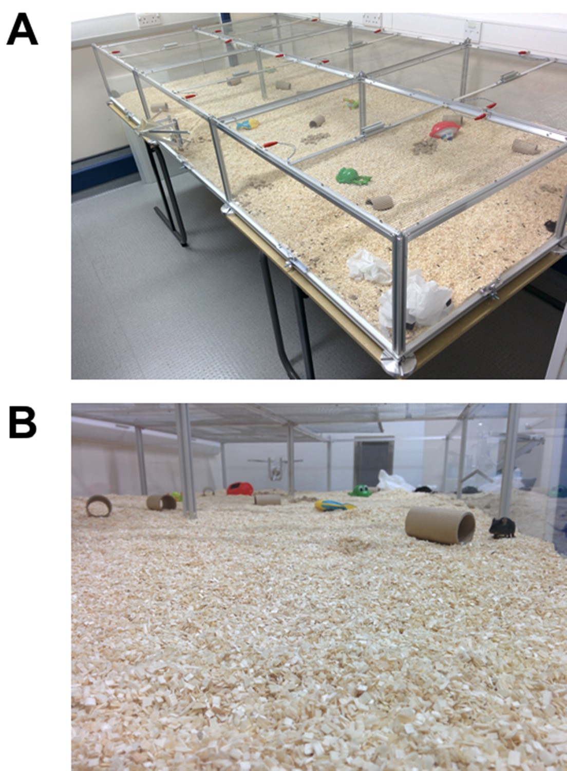
Large environment for housing.
(A, B) The large cage environment viewed from above (A) and from inside (B).
Figure 3
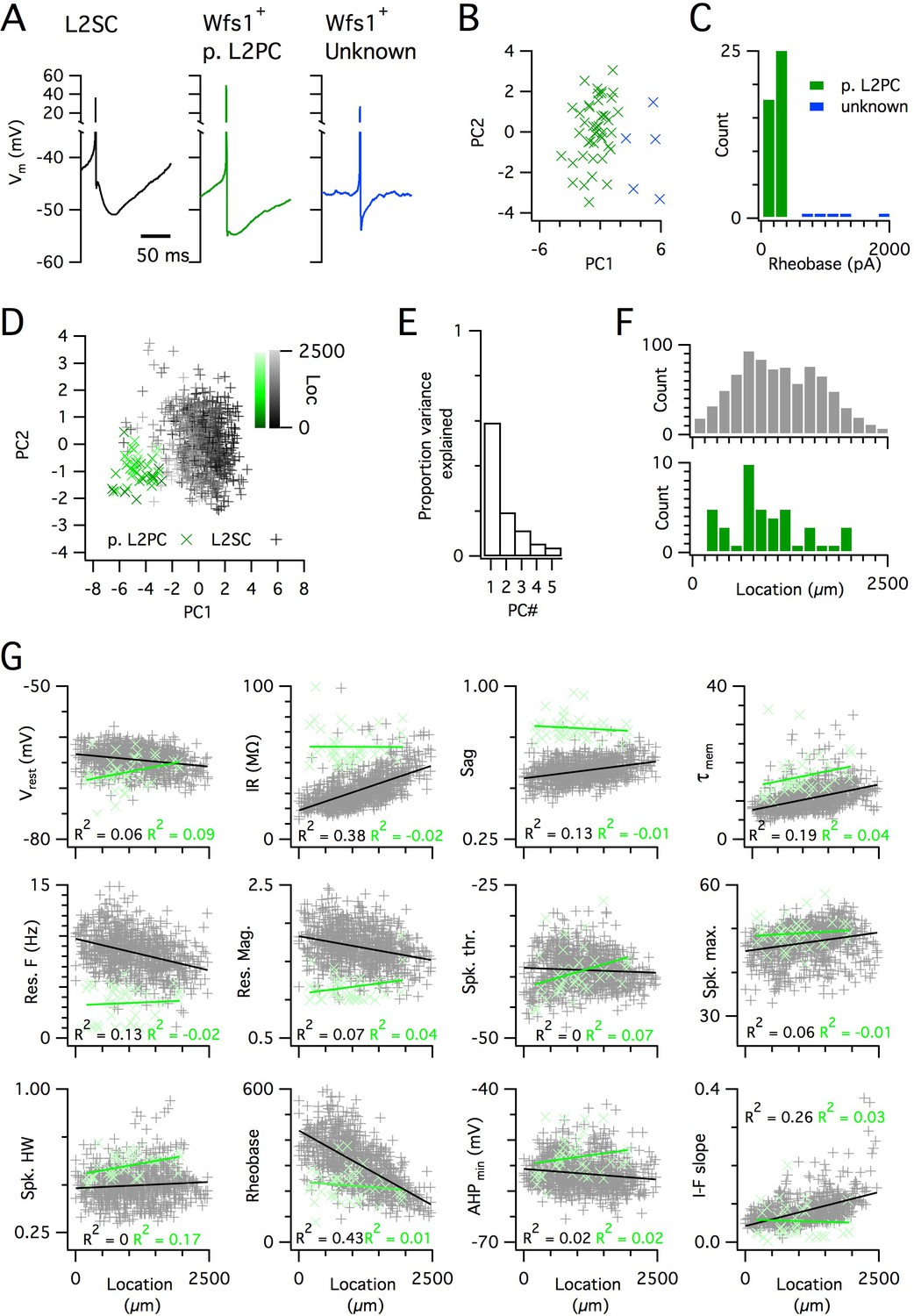
Distinct and dorsoventrally organized properties of layer 2 stellate cells.
(A) Representative action potential after hyperpolarization waveforms from a SC (left), a pyramidal cell (middle) and an unidentified cell (right). The pyramidal and unidentified cells were both positively labelled in Wfs1Cre mice. (B) Plot of the first versus the second principal component from PCA of the properties of labelled neurons in Wfs1Cre mice reveals two populations of neurons. (C) Histogram showing the distribution of rheobase values of cells positively labelled in Wfs1Cre mice. The two groups identified in panel (B) can be distinguished by their rheobase. (D) Plot of the first two principal components from PCA of the properties of the L2PC (n = 44, green) and SC populations (n = 836, black). Putative pyramidal cells (x) and SCs (+) are colored according to their dorsoventral location (inset shows the scale). (E) Proportion of total variance explained by the first five principal components for the analysis in panel (D). (F) Histograms of the locations of recorded SCs (upper) and L2PCs (lower). (G) All values of measured features from all mice are plotted as a function of the dorsoventral location of the recorded cells. Lines indicate fits of a linear model to the complete datasets for SCs (black) and L2PCs (green). Putative pyramidal cells (x, green) and SCs (+, black). Adjusted R2 values use the same color scheme.
Figure 4 with 1 supplement
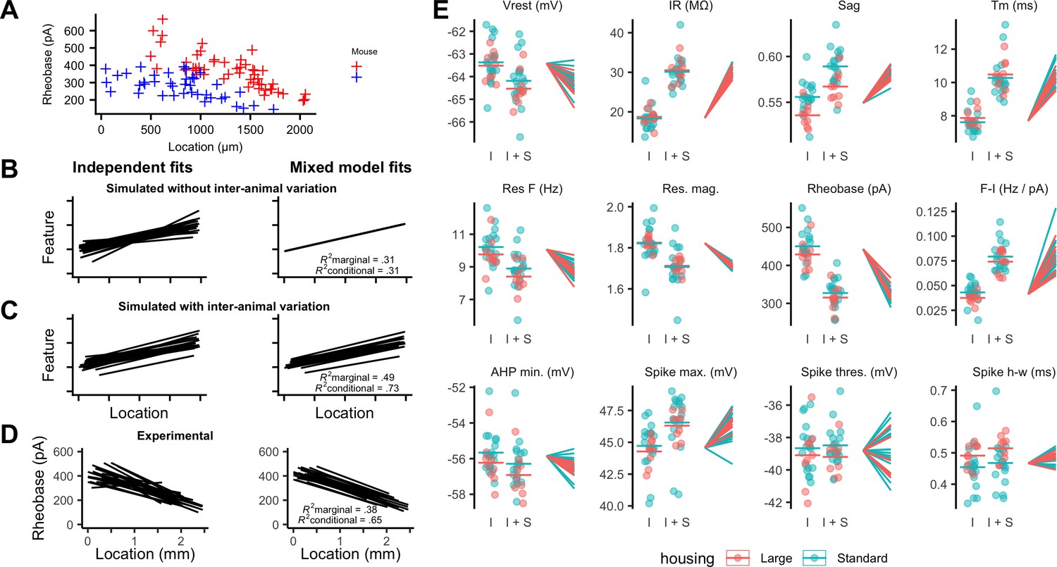
Inter-animal variability and dependence on environment of intrinsic properties of stellate cells.
(A) Examples of rheobase as a function of dorsoventral position for two mice. (B, C) Each line is the fit of simulated data from a different subject for datasets in which there is no inter-subject variability (B) or in which intersubject variability is present (C). Fitting data from each subject independently with linear regression models suggests intersubject variation in both datasets (left). By contrast, after fitting mixed effect models (right) intersubject variation is no longer suggested for the dataset in which it is absent (B) but remains for the dataset in which it is present (C). (D) Each line is the fit of rheobase as a function of dorsoventral location for a single mouse. The fits were carried out independently for each mouse (left) or using a mixed effect model with mouse identity as a random effect (right). (E) The intercept (I), sum of the intercept and slope (I + S), and slopes realigned to a common intercept (right) for each mouse obtained by fitting mixed effect models for each property as a function of dorsoventral position.
Figure 4—figure supplement 1
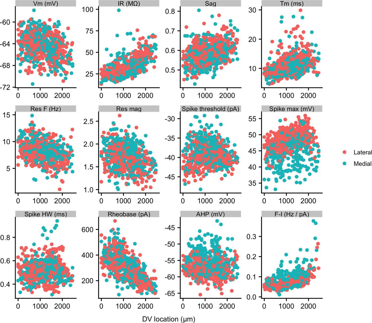
Properties of SCs in medial and lateral slices.
Membrane properties of SCs from slices containing more medial (blue) and more lateral (red) parts of the MEC plotted as a function of dorsal ventral position. Neurons from more medial slices had a higher spike threshold, a lower spike maximum and a less-negative spike after-hyperpolarization (see Supplementary file 6). Properties are labelled as in Figure 2.
Figure 5
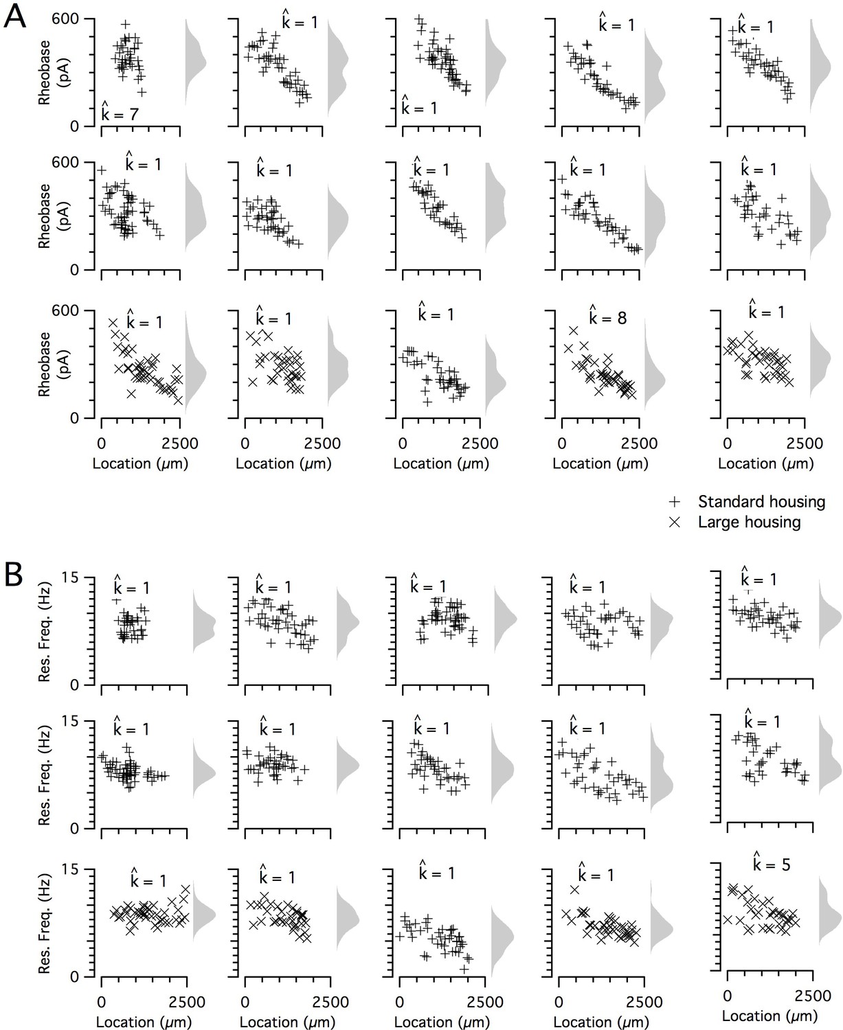
Rheobase and resonant frequency do not have a detectable modular organization.
(A, B) Rheobase (A) and resonant frequency (B) are plotted as a function of dorsoventral position separately for each animal. Marker color and type indicate the age and housing conditions of the animal (‘+’ standard housing, ‘x’ large housing). KSDs (arbitrary bandwidth, same for all animals) are also shown. The number of clusters in the data (kest) is indicated for each animal ().
Figure 6
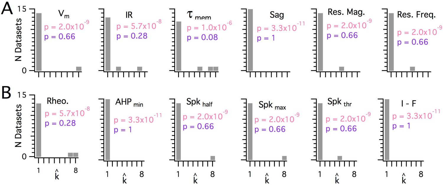
Significant modularity is not detectable for any measured property.
(A, B) Histograms showing the kest () counts across all mice for each different measured sub-threshold (A) and supra-threshold (B) intrinsic property. The maximum k evaluated was 8. The proportion of each measured property with kest>1 was compared using binomial tests (with N = 15) to the proportion expected if the underlying distribution of that property is always clustered with all separation between modes ≥5 standard deviations (pink text), or if the underlying distribution of the property is uniform (purple text). For all measured properties, the values of kest () were indistinguishable (p>0.05) from the data generated from a uniform distribution and differed from the data generated from a multi-modal distribution (p<1×10⁻⁶).
Figure 7
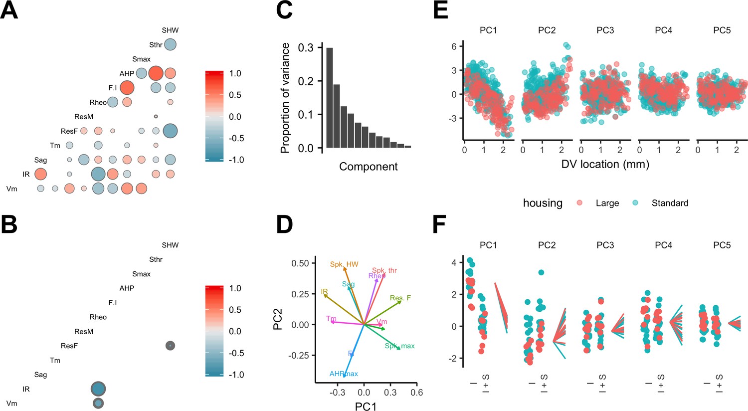
Feature relationships and inter-animal variability after reducing dimensionality of the data.
(A, B) Partial correlations between the electrophysiological features investigated at the level of individual neurons (A) and at the level of animals (B). Partial correlations outside of the 95% basic bootstrap confidence intervals are color coded. Non-significant correlations are colored white. Properties shown are the resting membrane potential (Vm), input resistance (IR), membrane potential sag response (sag), membrane time constant (Tm), resonance frequency (Rm), resonance magnitude (Rm), rheobase (Rheo), slope of the current frequency relationship (FI), peak of the action potential after hyperpolarization (AHP), peak of the action potential (Smax) voltage threshold for the action potential (Sthr) and half-width of the action potential (SHW). (C) Proportion of variance explained by each principal component. To remove variance caused by animal age and the experimenter identity, the principal component analysis used a reduced dataset obtained by one experimenter and restricted to animals between 32 and 45 days old (N = 25, n = 572). (D) Loading plot for the first two principal components. (E) The first five principal components plotted as a function of position. (F) Intercept (I), intercept plus the slope (I + S) and slopes aligned to the same intercept, for fits for each animal of the first five principal components to a mixed model with location as a fixed effect and animal as a random effect.
Figure 8
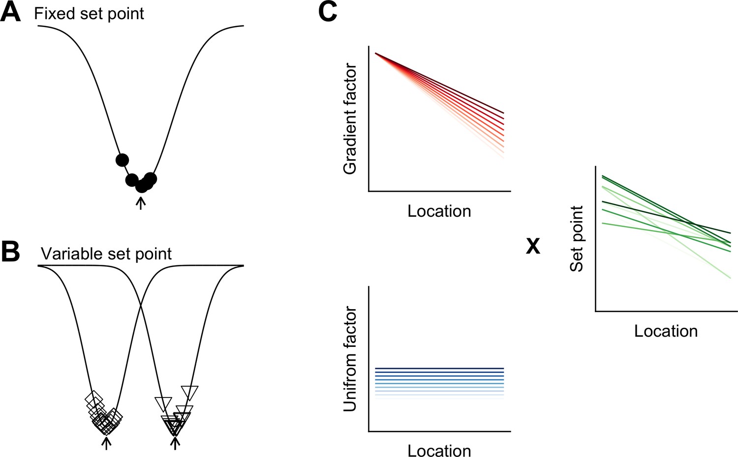
Models for intra- and inter-animal variation.
(A) The configuration of a cell type can be conceived of as a trough (arrow head) in a developmental landscape (solid line). In this scheme, the trough can be considered as a set point. Differences between cells (filled circles) reflect variation away from the set point. (B) Neurons from different animals or located at different dorsoventral positions can be conceptualized as arising from different troughs in the developmental landscape. (C) Variation may reflect inter-animal differences in factors that establish gradients (upper left) and in factors that are uniformly distributed (lower left), combining to generate set points that depend on animal identity and location (right). Each line corresponds to schematized properties of a single animal.
Author response image 1
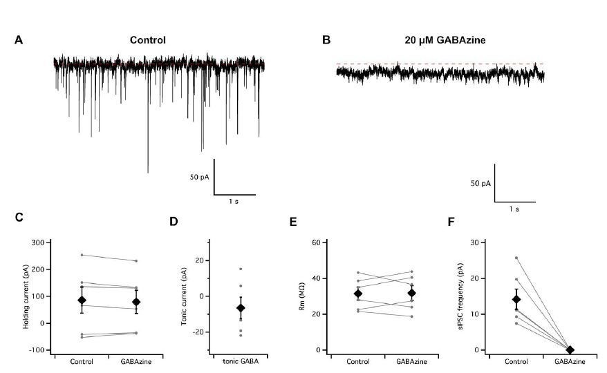
Absence of a tonic GABA-A receptor mediated input to entorhinal cortex stellate cells.
(A–B) Continuous voltage-clamp recording of spontaneous synaptic activity from a stellate cell in control conditions (A) and during perfusion of GABAzine to block GABA-A receptors (B). (C–D) Perfusion of GABAzine did not affect the holding current (C–D) or input resistance (E) but abolished fast spontaneous inhibitory currents (F).
Tables
Table 1
Dependence of the electrophysiological features of SCs on dorsoventral position.
Key statistical parameters from analyses of the relationship between each measured electrophysiological feature and dorsoventral location. The data are ordered according to the marginal R2 for each property’s relationship with dorsoventral position. Slope is the population slope from fitting a mixed effect model for each feature with location as a fixed effect (mm−1), with p(slope) obtained by comparing this model to a model without location as a fixed effect (χ2 test). For all properties except the spike thereshold, the slope was unlikely to have arisen by chance (p<0.05). The marginal and conditional R2 values, and the minimum and maximum slopes across all mice, are obtained from the fits of mixed effect models that contain location as a fixed effect. The estimate p(vs linear) is obtained by comparing the mixed effect model containing location as a fixed effect with a corresponding linear model without random effects (χ2 test). The values of p(slope) and p(vs linear) were adjusted for multiple comparisons using the method of Benjamini and Hochberg (1995). Units for the slope measurements are units for the property mm−1. The data are from 27 mice.
| Feature | Slope | P (slope) | Marginal R2 | Conditional R2 | Slope (min) | Slope (max) | P (vs linear) |
|---|---|---|---|---|---|---|---|
| IR (MΩ) | 11.794 | 8.39e-17 | 0.383 | 0.532 | 9.630 | 14.262 | 4.33e-40 |
| Rheobase (pA) | −119.887 | 9.07e-15 | 0.382 | 0.652 | −153.873 | −76.130 | 6.55e-43 |
| I-F slope (Hz/pA) | 0.036 | 6.06e-10 | 0.228 | 0.561 | 0.019 | 0.087 | 6.82e-34 |
| Tm (ms) | 2.646 | 3.70e-12 | 0.192 | 0.343 | 1.809 | 3.979 | 1.20e-29 |
| Res. frequency (Hz) | −1.334 | 4.13e-09 | 0.122 | 0.553 | −2.299 | −0.342 | 6.37e-65 |
| Sag | 0.033 | 6.06e-10 | 0.121 | 0.347 | 0.016 | 0.043 | 1.91e-38 |
| Spike maximum (mV) | 1.900 | 1.85e-05 | 0.064 | 0.436 | −1.288 | 3.297 | 1.14e-50 |
| Res. magnitude | −0.114 | 6.34e-08 | 0.064 | 0.198 | −0.138 | −0.087 | 9.13e-20 |
| Vm (mV) | −0.884 | 3.67e-05 | 0.046 | 0.348 | −1.965 | 0.150 | 8.73e-35 |
| Spike AHP (mV) | −0.645 | 1.93e-02 | 0.011 | 0.257 | −1.828 | 0.408 | 1.82e-17 |
| Spike width (ms) | 0.017 | 1.93e-02 | 0.010 | 0.643 | −0.021 | 0.055 | 7.04e-139 |
| Spike threshold (mV) | 0.082 | 8.20e-01 | 0.000 | 0.510 | −2.468 | 2.380 | 2.03e-17 |
Additional files
-
Supplementary file 1
Dependence of calbindin cell properties on dorsoventral position.
Analyses are as described for Table 1. Data are from GFP-positive putative pyramidal neurons (n = 42, N = 3).
- https://cdn.elifesciences.org/articles/52258/elife-52258-supp1-v4.docx
-
Supplementary file 2
Dependence of SC properties on age.
The distinguishing electrophysiological features of SCs and their dorsoventral organization were apparent at all ages, with some features depending significantly on age (left columns), consistent with the idea that SCs continue to mature beyond P18 (Boehlen et al., 2010; Burton et al., 2008). When we considered only animals between P33 and P44, we did not find any significant effect of age (right columns). Significance estimates for the effects of dorsoventral position (dvloc), age (age) and interactions between dorsoventral position and age (dvloc:age) were estimated using type II ANOVA and Wald χ2 test from fits to mixed models containing age and location as fixed effects and animal identity as random effects. Significance estimates were adjusted for multiple comparisons using the Benjamini and Hochberg method.
- https://cdn.elifesciences.org/articles/52258/elife-52258-supp2-v4.docx
-
Supplementary file 3
Dependence of SC properties on housing.
Analyses suggesting that the membrane potential sag, resonance frequency, and spike half-width of SCs differ between mice housed in standard and large home cages. Significance estimates for the effects of dorsoventral position (dvloc), housing (housing) and interactions between dorsoventral position and housing (dvloc:housing) estimated using type II ANOVA and Wald χ2 test from fits to mixed models containing age and location as fixed effects and animal identity as random effects. Initial significance estimates (raw p) were adjusted for multiple comparisons (adjusted p) using the Benjamini and Hochberg method.
- https://cdn.elifesciences.org/articles/52258/elife-52258-supp3-v4.docx
-
Supplementary file 4
Inter-animal differences in electrophysiological features remain after accounting for housing.
Results from comparison of a mixed effect model incorporating dorsoventral location and housing with an equivalent linear model. The significance estimate (p) is calculated using a χ2test and adjusted for multiple comparisons (p_adj) using the Benjamini and Hochberg method.
- https://cdn.elifesciences.org/articles/52258/elife-52258-supp4-v4.docx
-
Supplementary file 5
Dependence of SC properties on hemisphere.
We did not find significant effects of brain hemisphere on any features except for the relationship between dorsoventral location and sag. Significance estimates for the effects of dorsoventral position (dvloc), brain hemisphere (hemi) and interactions between dorsoventral position and hemisphere (dvloc:hemi) were estimated using type II ANOVA and Wald χ2 test from fits to mixed models containing age and location as fixed effects and animal identity as random effects. Initial significance estimates (raw p) were adjusted for multiple comparisons (adjusted p) using the Benjamini and Hochberg method.
- https://cdn.elifesciences.org/articles/52258/elife-52258-supp5-v4.docx
-
Supplementary file 6
Dependence of SC properties on mediolateral position.
Mediolateral as well as dorsoventral position has been reported to determine the sub-threshold electrophysiological features of SCs (Canto and Witter, 2012). We found significant effects of mediolateral position on all measured electrophysiological features. However, the sizes of the effects of mediolateral position on subthreshold features (vm, ir, sag, tau, resf, resmag, and rheo) were much smaller than for dorsoventral position. By contrast, supra-threshold features (spkthr, spkmax, and ahp) were more greatly affected by mediolateral position, with more medial neurons having a higher spike threshold, and lower amplitudes of the spike peak and of after-hyperpolarization. Fixed effects are the intercept and slope coefficients for mixed models containing dorsoventral and mediolateral location as fixed effects and animal identity as random effects. Significance estimates for the effects of dorsoventral position (dvloc), mediolateral position (ml) and interactions between dorsoventral position and mediolateral position (dvloc:ml) are estimated using type II ANOVA and Wald χ2 tests from the fits of the mixed models. Initial significance estimates (raw p) were adjusted for multiple comparisons (adjusted p) using the Benjamini and Hochberg method.
- https://cdn.elifesciences.org/articles/52258/elife-52258-supp6-v4.docx
-
Supplementary file 7
Dependence of SC properties on experimenter.
We found that for many electrophysiological features, the identity of the experimenter affected the intercept, but not the slope, of their relationship with dorsoventral position. All features except for spike threshold nevertheless followed a dorsoventral organization after accounting for the experimenter. Significance estimates for the effects of dorsoventral position (dvloc), experimenter (exp) and interactions between dorsoventral position and experimenter (dvloc:exp) were estimated using type II ANOVA and Wald χ2 tests from fits to mixed models containing age and location as fixed effects and animal identity as random effects. Initial significance estimates (raw p) were adjusted for multiple comparisons (adjusted p) using the Benjamini and Hochberg method.
- https://cdn.elifesciences.org/articles/52258/elife-52258-supp7-v4.docx
-
Supplementary file 8
Dependence of SC properties on time since slice preparation.
We anticipated that the interval between slice preparation and recording may influence the measured electrophysiological features. Consistent with our expectation, analyses of the data were consistent with changes to some electrophysiological features of SCs with time since slice preparation, but dorsoventral gradients could not be explained by these changes. Significance estimates for the effects of dorsoventral position (dvloc), time since slice preparation (rect) and interactions between dorsoventral position and experimenter (dvloc:rect) estimated using type II ANOVA and Wald χ2 tests from fits to mixed models containing age and location as fixed effects and animal identity as random effects. Initial significance estimates (raw p) were adjusted for multiple comparisons (adjusted p) using the Benjamini and Hochberg method.
- https://cdn.elifesciences.org/articles/52258/elife-52258-supp8-v4.docx
-
Supplementary file 9
Dependence of SC properties on direction in which sequential recordings are made.
In anticipation of the effects of the time since slice preparation on the electrophysiological features of SCS, we varied the direction along the dorsoventral axis from which consecutive recordings were made between experimenters and experimental days (see 'Materials and methods'). Consistent with effects of time on electrophysiological features (see Supplementary file 7 above), we found that the direction in which sequential recordings were made influenced the slope, but not the intercept of several electrophysiological features. Significance estimates for the effects of dorsoventral position (dvloc), direction in which sequential recordings were made (dir) and interactions between dorsoventral position and recording direction (dvloc:dir) estimated using type II ANOVA and Wald χ2 tests from fits to mixed models containing age and location as fixed effects and animal identity as random effects. Initial significance estimates (raw p) were adjusted for multiple comparisons (adjusted p) using the Benjamini and Hochberg method.
- https://cdn.elifesciences.org/articles/52258/elife-52258-supp9-v4.docx
-
Supplementary file 10
Inter-animal differences in extended models.
Results from comparison of a mixed effect model incorporating dorsoventral location, housing, mediolateral position, experimenter identity and direction in which recordings were obtained with an equivalent linear model. Data are from animals between 32 and 45 days old. The significance estimate (p) is calculated using a χ2 test and adjusted for multiple comparisons (p_adj) using the Benjamini and Hochberg method.
- https://cdn.elifesciences.org/articles/52258/elife-52258-supp10-v4.docx
-
Supplementary file 11
Inter-animal differences in models fit to minimal datasets.
Results from comparison of mixed effect models with dorsoventral location as a fixed effect and animal identity as a random effect using minimal datasets obtained by either HP (upper) or DG (lower). Data are from animals between 32 and 45 days old. Because of the smaller size of these datasets, the statistical power to detect inter-animal variation is reduced. Nevertheless, in these analyses, the conditional R2 of the mixed model fit was again substantially higher than the marginal R2, and most (9/12) features were better fit by a mixed model compared to a corresponding linear model in both datasets.
- https://cdn.elifesciences.org/articles/52258/elife-52258-supp11-v4.docx
-
Supplementary file 12
Electrophysiological features and the number of recorded neurons.
Significance estimates for the effects of dorsoventral position (dvloc), number of recorded neurons (counts) and interactions between dorsoventral position and number of recorded neurons (dvloc:counts) estimated using type II ANOVA and Wald χ2 tests from fits to mixed models containing age and location as fixed effects and animal identity as random effects. Initial significance estimates (raw p) were adjusted for multiple comparisons (adjusted p) using the Benjamini and Hochberg method.
- https://cdn.elifesciences.org/articles/52258/elife-52258-supp12-v4.docx
-
Supplementary file 13
Inter-animal differences for experiments with >35 recorded neurons.
Analyses of inter-animal differences focusing only on data from animals for which > 35 recordings were made (N = 11, n = 459). Comparison of marginal and conditional R2 values continued to indicate substantial inter-animal variance, and fits obtained with mixed models remained significantly different to fits that did not account for animal identity (p<4.4×10⁻⁵). Analyses are as for Supplementary file 1, but are restricted to experiments in which > 35 neurons were recorded from.
- https://cdn.elifesciences.org/articles/52258/elife-52258-supp13-v4.docx
-
Supplementary file 14
Dependence of principal components on dorsoventral position and animal identity.
Analyses are as described for Table 1, but were applied to principal components of the electrophysiological features of SCs.
- https://cdn.elifesciences.org/articles/52258/elife-52258-supp14-v4.docx
-
Supplementary file 15
Dependence of principal components of SC properties on housing.
Analyses are as described for Supplementary file 3, but are applied to principal components of the electrophysiological features of SCs.
- https://cdn.elifesciences.org/articles/52258/elife-52258-supp15-v4.docx
-
Supplementary file 16
Dependence of principal components on animal identity in models that account for housing.
Analyses are as for Supplementary file 10, but are applied to principal components of the electrophysiological features of SCs.
- https://cdn.elifesciences.org/articles/52258/elife-52258-supp16-v4.docx
-
Transparent reporting form
- https://cdn.elifesciences.org/articles/52258/elife-52258-transrepform-v4.docx
Download links
A two-part list of links to download the article, or parts of the article, in various formats.
Downloads (link to download the article as PDF and Executable version)
Open citations (links to open the citations from this article in various online reference manager services)
Cite this article (links to download the citations from this article in formats compatible with various reference manager tools)
Inter- and intra-animal variation in the integrative properties of stellate cells in the medial entorhinal cortex
eLife 9:e52258.
https://doi.org/10.7554/eLife.52258


