Dopamine role in learning and action inference
- MRC Brain Networks Dynamics Unit, University of Oxford, United Kingdom
Figures
Figure 1
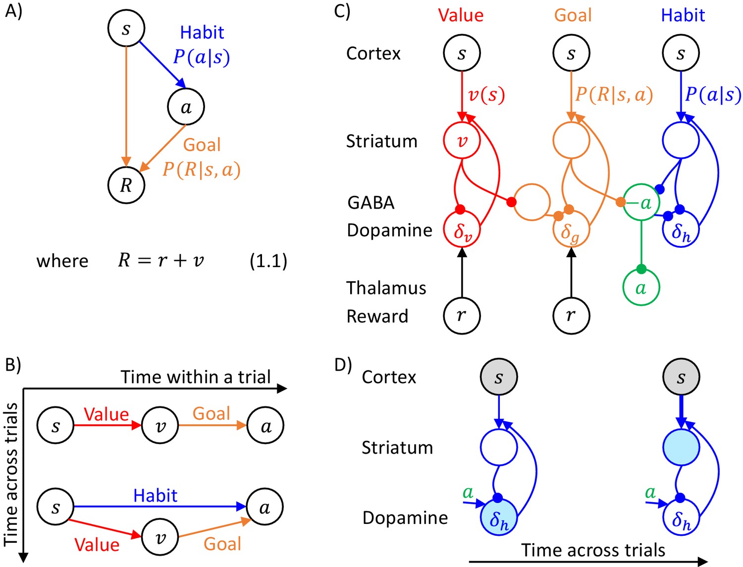
Overview of systems within the DopAct framework.
(A) Probabilistic model learned by the actor. Random variables are indicated by circles, and arrows denote dependencies learned by different systems. (B) Schematic overview of information processing in the framework at different stages of task acquisition. (C) Mapping of the systems on different parts of the cortico-basal ganglia network. Circles correspond to neural populations located in the regions indicated by labels to the left, where ‘Striatum’ denotes medium spiny neurons expressing D1 receptors, ‘GABA’ denotes inhibitory neurons located in vicinity of dopaminergic neurons, and ‘Reward’ denotes neurons providing information on the magnitude of instantaneous reward. Arrows denote excitatory projections, while lines ending with circles denote inhibitory projections. (D) Schematic illustration of the mechanism of habit formation. Notation as in panel C, but additionally shading indicates the level of activity, and thickness of lines indicates the strength of synaptic connections.
Figure 2

Schematic illustration of changes in dopaminergic activity in the goal-directed system while a hungry rat presses a lever and a food pellet is delivered.
(A) Prediction error reduced by action planning. The prediction error encoded in dopamine (bottom trace) is equal to a difference between the reward available (top trace) and the expectation of reward arising from a plan to obtain it (middle trace). (B) Prediction errors reduced by both action planning and learning.
Figure 3
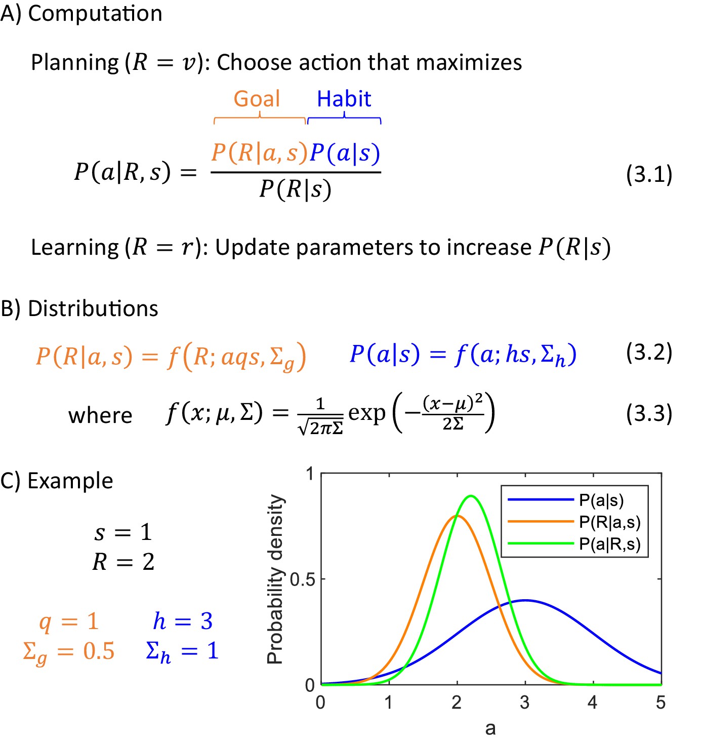
Computational level.
(A) Summary of computations performed by the actor. (B) Sample form of probability distributions. (C) An example of inference of action intensity. In this example the stimulus intensity is equal to , the valuation system computes desired reward , and the parameters of the probability distributions encoded in the goal-directed and habit systems are listed in the panel. The blue curve shows the distribution of action intensity, which the habit system has learned to be generally suitable for this stimulus. The orange curve shows probability density of obtaining reward of 2 for a given action intensity, and this probability is estimated by the goal-directed system. For the chosen parameters, it is the probability of obtaining 2 from a normal distribution with mean . Finally, the green curve shows a posterior distribution computed from Equation 3.1.
Figure 4
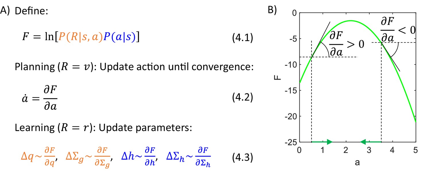
Algorithmic level.
(A) Summary of the algorithm used by the actor. (B) Identifying an action based on a gradient of . The panel shows an example of a dependence of on , and we wish to take the value maximizing . To find the action, we let to change over time in proportion to the gradient of over (Equation 4.2, where the dot over denotes derivative over time). For example, if the action is initialized to .5, then the gradient of at this point is positive, so is increased (Equation 4.2), as indicated by a green arrow on the x-axis. These changes in continue until the gradient is no longer positive, i.e. when is at the maximum. Analogously, if the action is initialized to , then the gradient of is negative, so is decreased until it reaches the maximum of .
Figure 5
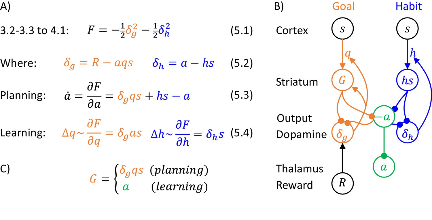
Description of a model selecting action intensity, in a case of unit variances.
(A) Details of the algorithm. (B) Mapping of the algorithm on network architecture. Notation as in Figure 1C, and additionally ‘Output’ denotes the output nuclei of the basal ganglia. (C) Definition of striatal activity in the goal-directed system.
Figure 6
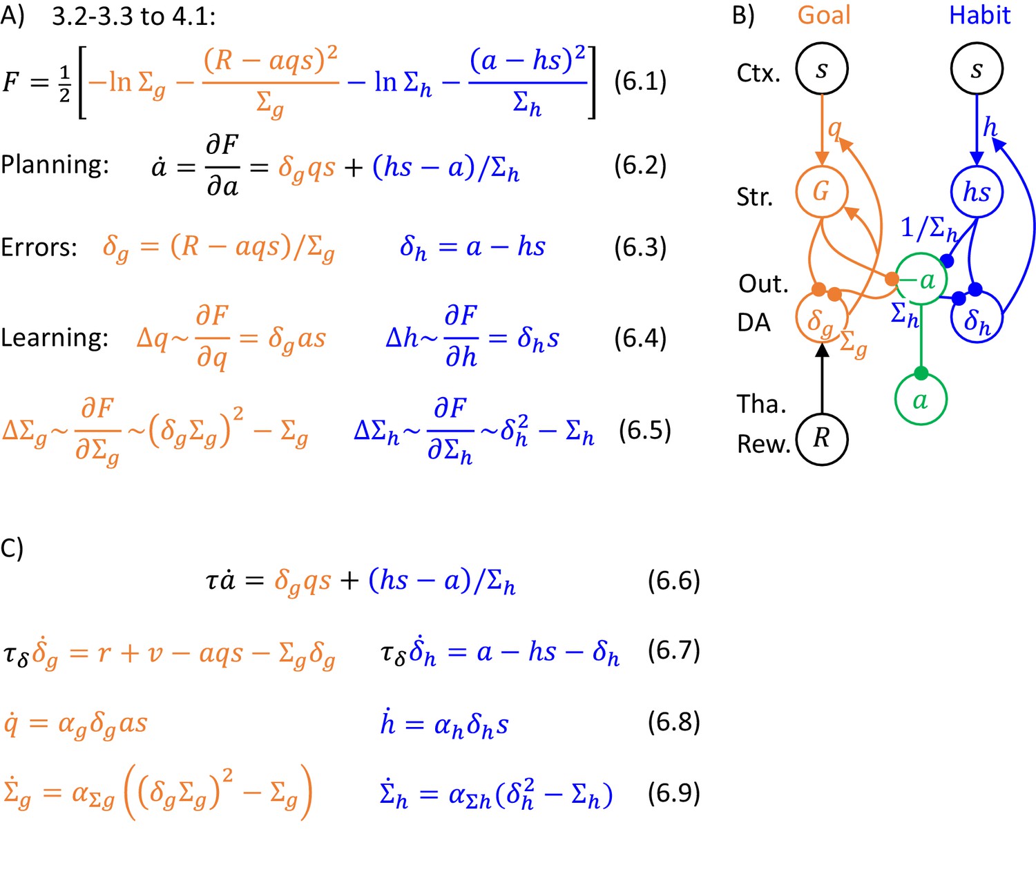
Description of a model selecting action intensity.
(A) Details of the algorithm. The update rules for the variance parameters can be obtained by computing derivatives of , giving and but to simplify these expressions, we scale them by and , resulting in Equations 6.5. Such scaling does not change the value to which the variance parameters converge because and are positive. (B) Mapping of the algorithm on network architecture. Notation as in Figure 5B. This network is very similar to that shown in Figure 5B, but now the projection to output nuclei from the habit system is weighted by its precision (to reflect the weighting factor in Equation 6.2), and also the rate of decay (or relaxation to baseline) in the output nuclei needs to depend on . One way to ensure that the prediction error in goal-directed system is scaled by is to encode in the rate of decay or leak of these prediction error neurons (Bogacz, 2017). Such decay is included as the last term in orange Equation 6.7 describing the dynamics of prediction error neurons. Prediction error evolving according to this equation converges to the value in orange Equation 6.3 (the value in equilibrium can be found by setting the left hand side of orange Equation 6.7 to 0, and solving for ). In Equation 6.7, total reward was replaced according to Equation 1.1 by the sum of instantaneous reward , and available reward computed by the valuation system. (C) Dynamics of the model.
Figure 7

Simulation of a model selecting action intensity.
(A) Mean reward given to a simulated agent as a function of action intensity. (B) Changes in variables encoded by the valuation system in different stages of task acquisition. (C) Changes in variables encoded by the actor. (D) Changes in model parameters across trials. The green curve in the right display shows the action intensity at the end of a planning phase of each trial. (E) Action intensity inferred by the model after simulated blocking of dopaminergic neurons.
Figure 8
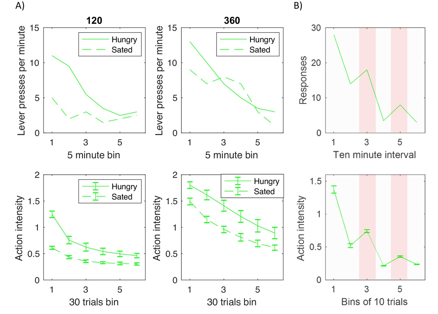
Comparison of experimentally observed lever pressing (top displays) and action intensity produced by the model (bottom displays).
(A) Devaluation paradigm. Top displays replot data represented by open shapes in Figure 1 in a paper by Dickinson et al., 1995. Bottom displays show the average action intensity produced by the model across bins of 30 trials of the testing period. Simulations were repeated 10 times, and error bars indicate standard deviation across simulations. (B) Pavlovian-instrumental transfer. Top display replots the data represented by solid line in Figure 1 in a paper by Estes, 1943. Bottom displays show the average action intensity produced by the model across bins of 10 trials of the testing period. Simulations were repeated 10 times, and error bars indicate standard error across simulations.
Figure 9
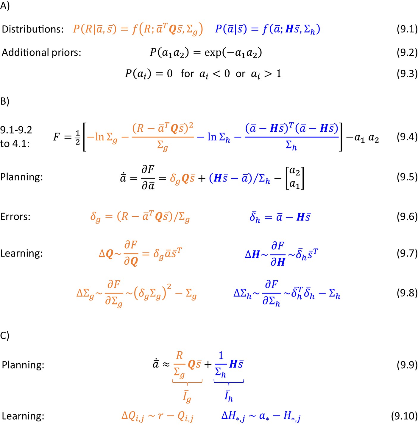
Description of the model of choice between two actions.
(A) Probability distributions assumed in the model. (B) Details of the algorithm. (C) Approximation of the algorithm. In blue Equation 9.10, * indicates that the parameters are updated for all actions.
Figure 10
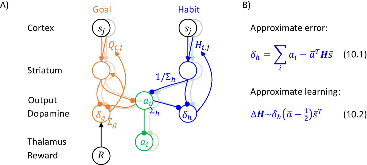
Implementation of the model of choice between two actions.
(A) Mapping of the algorithm on network architecture. Notation as in Figure 5B. (B) An approximation of learning in the habit system.
Figure 11
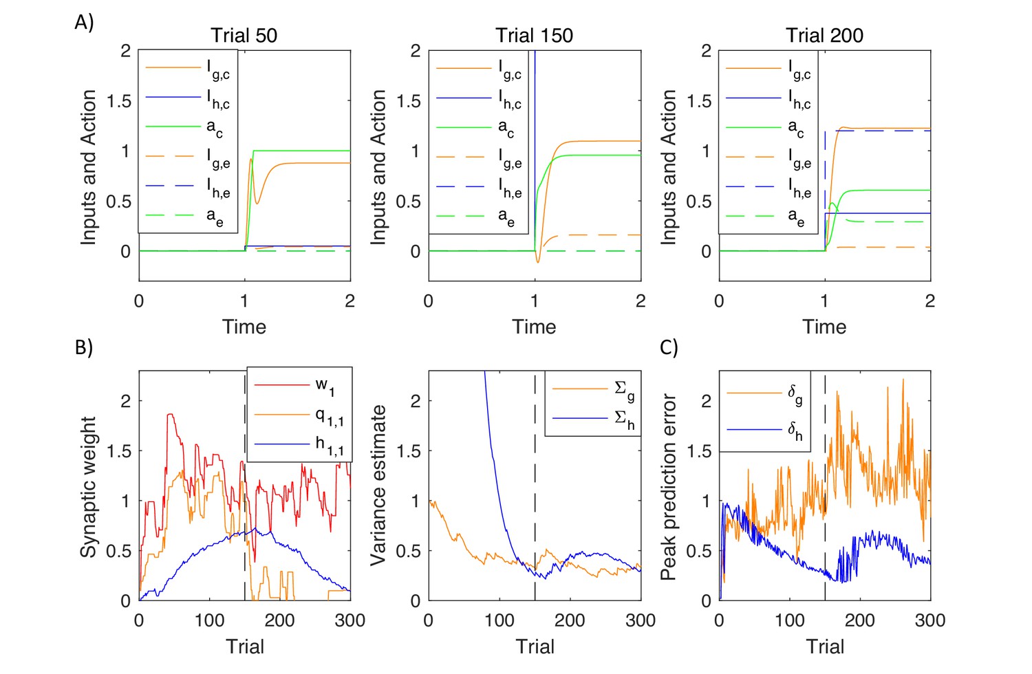
Simulation of the model of choice between two actions.
(A) Changes in action intensity and inputs from the goal-directed and habit systems, defined below Equation 9.9. Solid lines correspond to a correct action and dashed lines to an error. Thus selecting action 1 for stimulus 1 (or action 2 for stimulus 2) corresponds to solid lines before reversal (left and middle displays) and to dashed lines after reversal (right display). (B) Changes in model parameters across trials. Dashed black lines indicate a reversal trial. (C) Maximum values of prediction errors during action planning on each simulated trial.
Figure 12
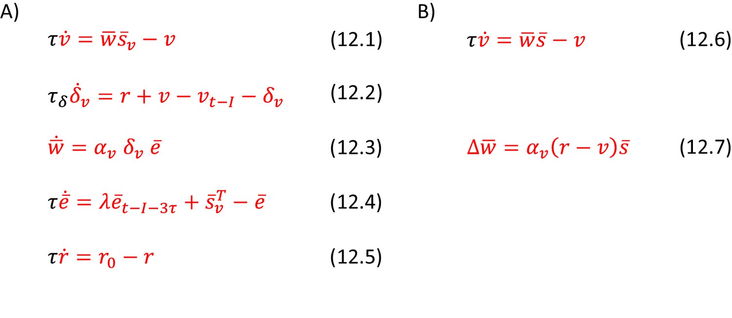
Description of the valuation system.
(A) Temporal difference learning model used in simulations of action intensity selection. (B) A simplified model used in simulations of choice between two actions.
Additional files
Download links
A two-part list of links to download the article, or parts of the article, in various formats.
Downloads (link to download the article as PDF)
Open citations (links to open the citations from this article in various online reference manager services)
Cite this article (links to download the citations from this article in formats compatible with various reference manager tools)
Dopamine role in learning and action inference
eLife 9:e53262.
https://doi.org/10.7554/eLife.53262


