The dynamic transmission of positional information in stau- mutants during Drosophila embryogenesis
- State Key Laboratory of Nuclear Physics and Technology & Center for Quantitative Biology, Peking University, China
- China National Center for Biotechnology Development, China
Figures
Figure 1 with 8 supplements
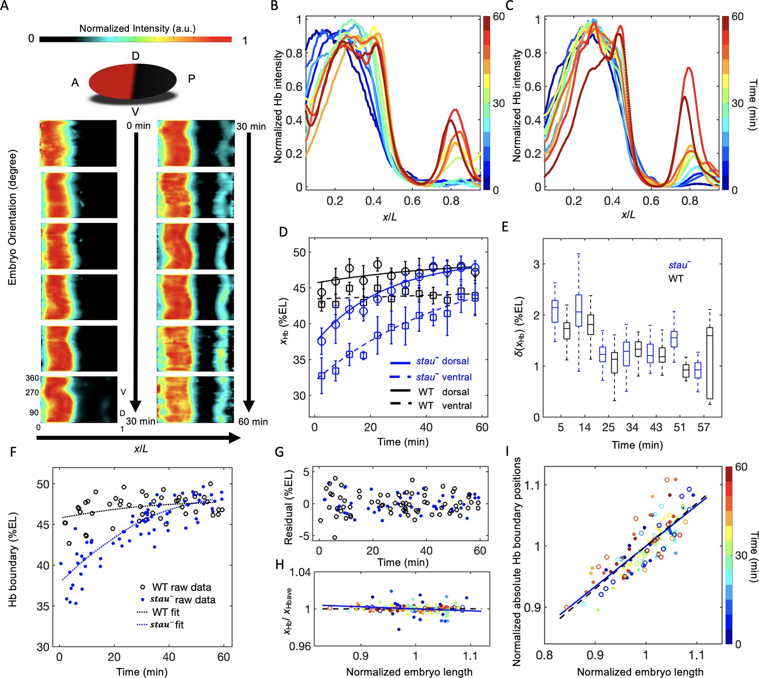
The Hb boundary reproducibly moves posteriorly in a much larger range in stau– mutants than in the WT based on 3D imaging.
(A) Heat map of the normalized Hb intensity in stau– mutants with a time-step of 5 min in nc14 based on projection at different angles along the AP axis from the 3D imaging on embryos. (B, C) Dynamics of the average dorsal Hb profiles extracted from 3D imaging of the embryos of stau– mutants (B) and the WT (C) in nc14. (D) The average Hb boundary position (xHb) in each 5 min bin of stau– mutants (blue) and the WT (black) as a function of the developmental time in nc14. Each circle (square) represents the average of the dorsal (ventral) boundary positions of Hb in the bin, and error bars denote the standard deviation of the bin. Lines are eye guides. (E) The variability of the Hb boundary in each bin with equal sample numbers of stau– mutants (blue, n = 10 in each bin except the last one) and the WT (black, n = 7 in each bin except the last one) as a function of the developmental time in nc14. Error bars are calculated from bootstrapping. (F, G) De-trend analysis of the Hb boundary. When we used smooth splines to fit the Hb boundary of all the measured embryos as a function of the embryo development time into nc14 (F), the fitting residuals (G) for the stau– mutants (blue) and the WT (black) are comparable with each other. The standard deviations of the residual are 1.67% EL (n = 69) and 1.45% EL (n = 47) for stau– mutants and the WT, respectively. Two-sample F-test for equal variances cannot be rejected (p=0.31). (H, I) Scaling analysis of the Hb boundary. The plots show normalized relative Hb boundary position (H) or normalized absolute Hb boundary positions with respect to the anterior pole (I) versus normalized embryo length for stau– mutants (solid circles, solid line) and the WT (open circles, dashed line). The slopes of the linear regression lines fitting to all the data points for the WT and stau– mutants are 0.0004 (R2 = 0.0003, n = 47) and −0.02 (R2 = 0.028, n = 69), respectively (H), or 0.70 (R2 = 0.69, n = 47) and 0.66 (R2 = 0.66, n = 69), respectively (I). Each embryo length is normalized by the average embryo length of all embryos. The Hb boundary position is normalized by the corresponding fitting value in the de-trend analysis (F).
-
Figure 1—source data 1
Average Hb profiles and single embryo boundary positions.
- https://cdn.elifesciences.org/articles/54276/elife-54276-fig1-data1-v2.xlsx
-
Figure 1—source data 2
The dynamics of the average and variability of Hb boundaries with equal sample size binning.
Source data for Figure 1E.
- https://cdn.elifesciences.org/articles/54276/elife-54276-fig1-data2-v2.docx
Figure 1—figure supplement 1
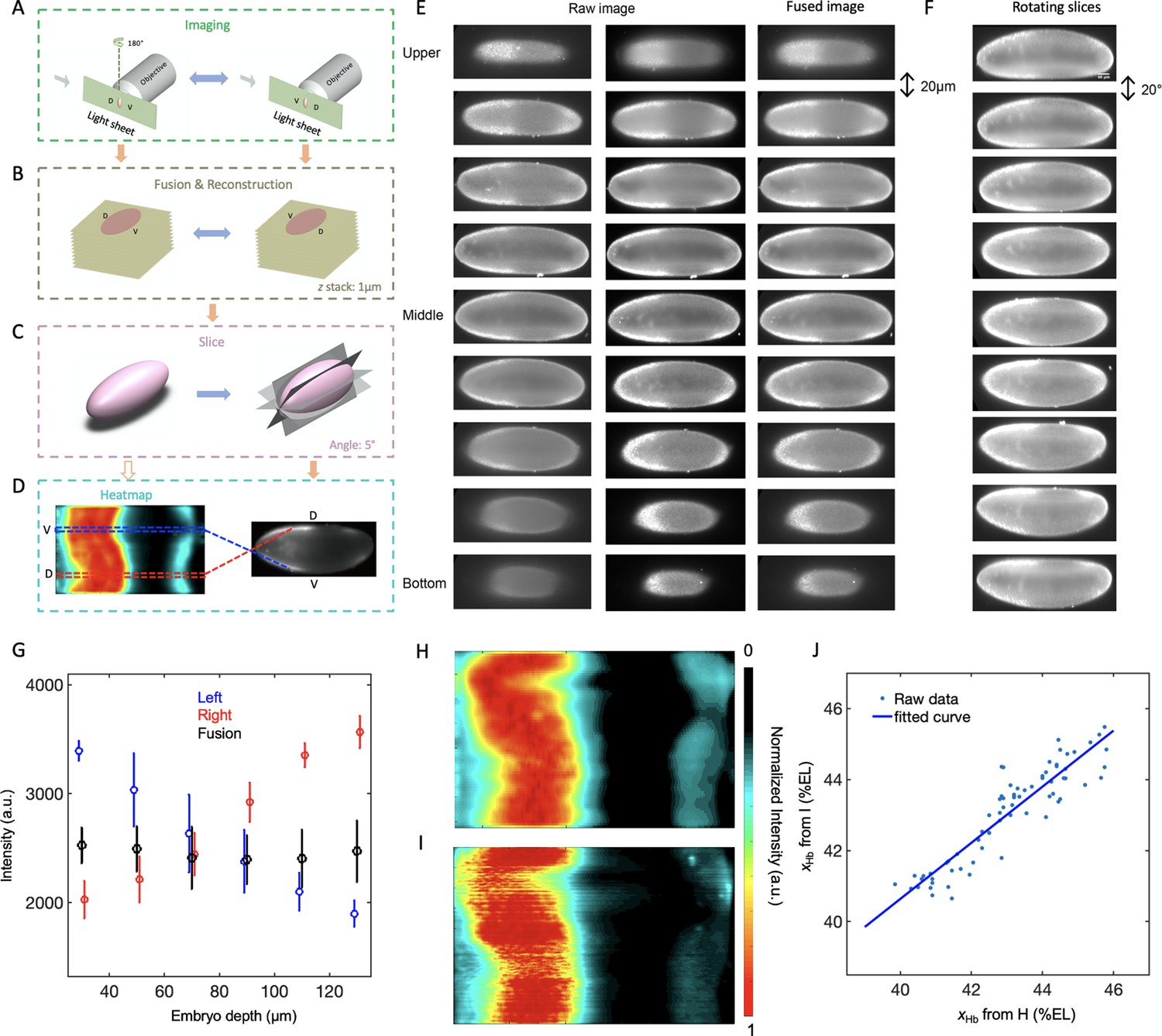
3D imaging measurement procedure.
(A) Each embryo was rotated 180° so that it could be imaged from two opposite directions with a light-sheet microscope. (B) The resultant z-stacks were corrected for intensity decay as a function of the depth then fused together to reconstruct a 3D embryo. (C) The expression profiles were extracted from the 2D plane rotating along the A-P axis of the embryo. (D) These profiles were normalized with the maximum intensity of the whole embryo and assembled to form the final heat map (left). The dorsal and ventral profiles are extracted from a representative lateral view of the embryo image (right) sliced from the reconstructed 3D embryo. (E) A subset of raw images of a typical embryo taken with the light-sheet microscope from both directions (the penetration depth increases and decreases for the first and second column, respectively), after image fusion, and after projection at different angles. The bright spots on the surface of the embryos are the clustered fluorescence beads. (F) Intensity compensation on the imaging depth by fusing the images taken from two opposite directions with a light-sheet microscope. (G–I) Comparison of heat map generation methods. A representative heat map of the Hb profiles of the WT generated with our method (G) is comparable with that generated using ImSAnE (Image Surface Analysis Environment) (Heemskerk and Streichan, 2015) (H). The Hb boundary positions extracted from the two heat maps are consistent with each other (I). The standard deviation of the residual from the linear fit in the scatter plot (I) is 0.6% EL.
Figure 1—figure supplement 2

Age determination of fixed Drosophila embryos.
(A) The depth of the membrane furrow canal (FC) on the dorsal side of the w1118 embryos measured with live imaging as a function of the developmental time into nc14 (t). Each gray line represents the curve of FC versus t measured for one embryo. The average curve of FC versus t of five w1118 embryos (black line) is slightly different from that of Oregon-R (Dubuis et al., 2013) (dashed line). The inset shows a middle dorsal part of a representative image of a live w1118 embryo and the corresponding FC. (B) The calculated depth of the membrane FC on the dorsal side of the fixed w1118 embryos with a shrinkage ratio of 94% as a function of the developmental time into nc14 (t). The inset shows the error in determining the embryo age of fixed embryos with the measured curve of FC versus t.
Figure 1—figure supplement 3
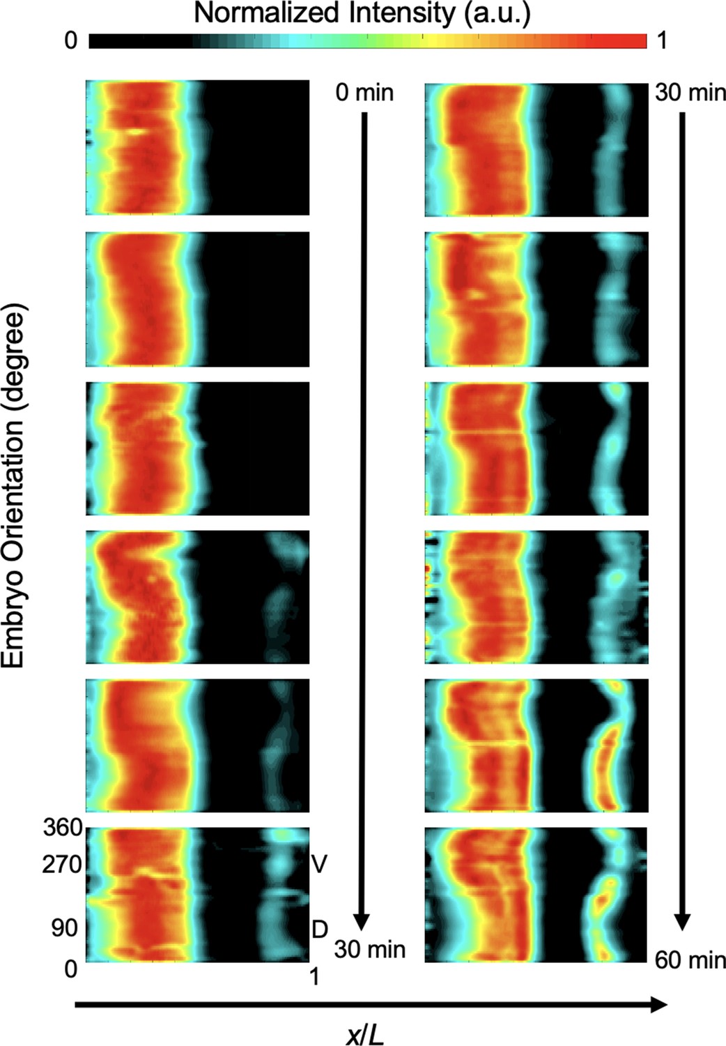
Heat map of the Hb profiles of the WT taken from the projection.
Figure 1—figure supplement 4
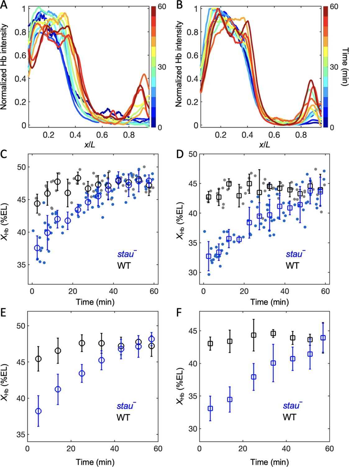
Dynamics of Hb profiles in stauHL54 mutants.
(A, B) The dynamics of the average ventral Hb profiles extracted from 3D imaging of the embryos of the WT (A) and stau– mutants (B). (C, D) Average dorsal (C) and ventral (D) Hb boundary position (xHb) in each 5 min bin of stau– mutants (blue circle) and the WT (black circle) as a function of the developmental time in nc14, error bars denote the standard deviation of the bin; each dot represents the boundary position of a single embryo. (E,F) Average dorsal (E) and ventral (F) xHb in each bin with the same sample size (n=10 and 7 except the last bin for stau- mutants and the WT, respectively) of stau- mutants (blue circle) and the WT (black circle) as a function of the developmental time in nc14, error bars denote the standard deviation of the bin.
Figure 1—figure supplement 5
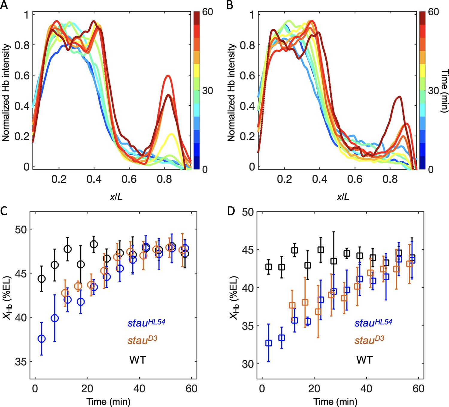
Dynamics of Hb profiles in stauD3 mutants.
(A. B) The dynamics of the average dorsal (A) and ventral (B) Hb profiles extracted from 3D imaging of the embryos of stauD3 mutants (n = 61). (C,D) Average dorsal (C) and ventral (D) Hb boundary position (xHb) in each 5 min bin of stauD3 mutants (orange circle), stauHL54 mutants (blue circle), and the WT (black circle) as a function of the developmental time in nc14. Error bars denote the standard deviation of each bin.
Figure 1—figure supplement 6

Dependence of xHb variability on spatial and temporal measurement errors.
(A, B) The variability of xHb extracted from the dorsal, ventral and symmetric profiles as a function of the embryo orientation along the AP axis at 16 min into nc14 (A) and 40 min into nc14 (B). (C, D) All of the Hb dorsal profiles without any control on embryo ages and orientations (C), and Hb dorsal profiles with an embryo age of 30–50 min and spatial orientation errors of less than 30° (D).
Figure 1—video 1
The z-stack of the immunofluorescence images of DAPI of the representative stau– mutant embryo after fusion in 3D imaging.
Figure 1—video 2
The z-stack of the immunofluorescence images of Hb of the representative stau– mutant embryo after fusion in 3D imaging.
Figure 2 with 1 supplement

The Bcd gradient noise of stau– mutants is comparable with that of the WT.
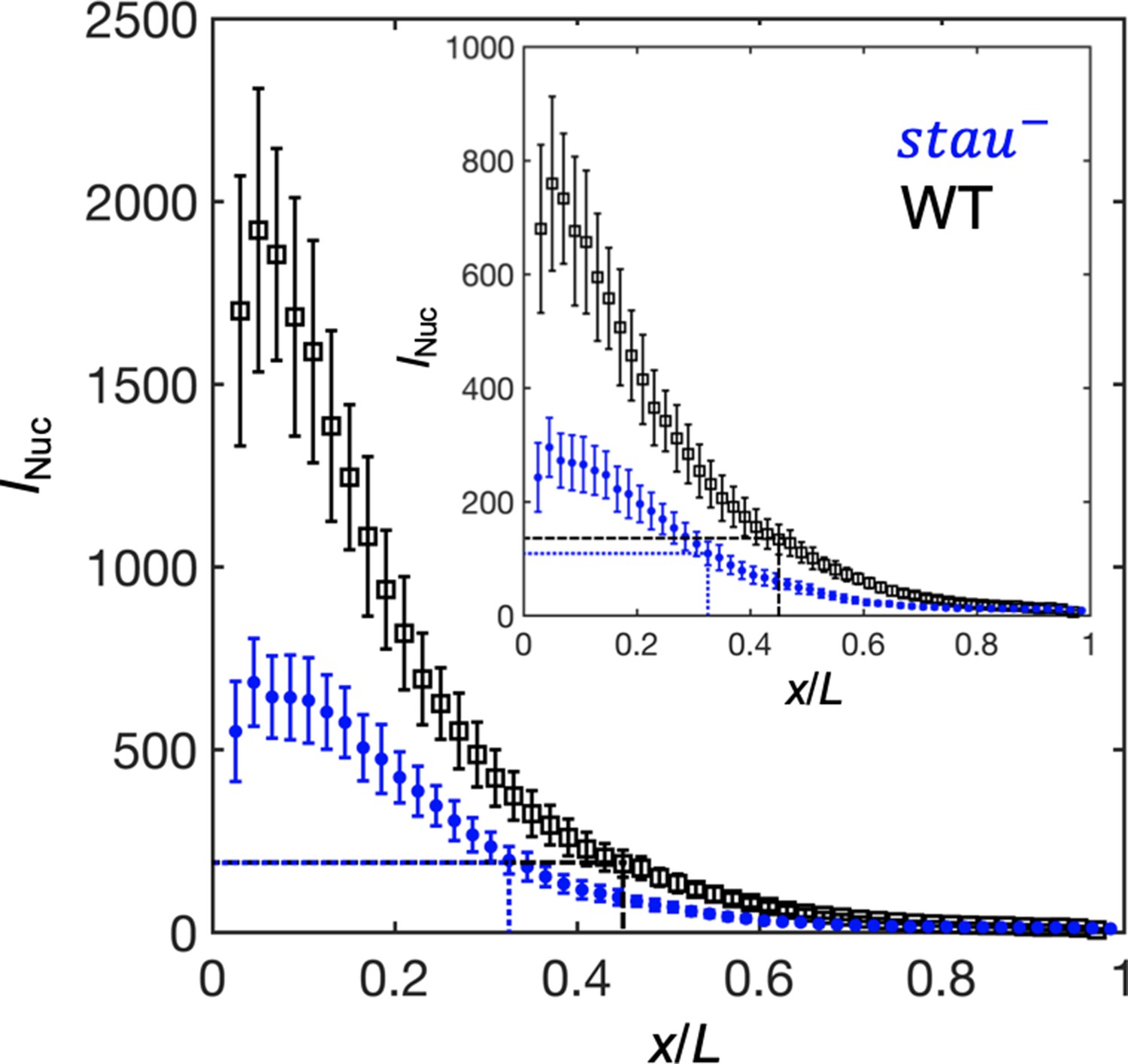
(A) The average intensity of the nuclear Bcd-GFP gradient of stau– mutants (blue) and the WT (black) as a function of the fractional embryo length at 16 min into nc14. Each circle and error bar represents the average and standard deviation, respectively, of the Bcd-GFP fluorescence intensity of the nuclei in the bin with a bin size of 2% EL. The inset shows the logarithm of the intensity as a function of the fractional embryo length and the linear fit in the range of 0.1–0.8 EL. (B) The relative Bcd-GFP gradient noise of stau– mutants (blue) and the WT (black). Each circle represents the standard deviation divided by the mean of the Bcd-GFP fluorescence intensity of the nuclei in the bin with a bin size of 2% EL. The error bar represents the standard deviation of the mean relative gradient noise calculated with bootstrap. (C) Variation in the average profiles of the Bcd gradient in stau– mutants from nc12 to 50 min into nc14. (D, E) The heat map of the Bcd gradient noise of the WT (D) and stau– mutants (E) from nc12 to 50 min into nc14. (F) The average Bcd gradient noise of stau– mutants from x = 0 to x = 0.55 EL versus developmental time is comparable with that of the WT.
-
Figure 2—source data 1
Bcd gradients measured at 16 min into nc14.
Source data for Figure 2A and B.
- https://cdn.elifesciences.org/articles/54276/elife-54276-fig2-data1-v2.xlsx
Figure 2—figure supplement 1
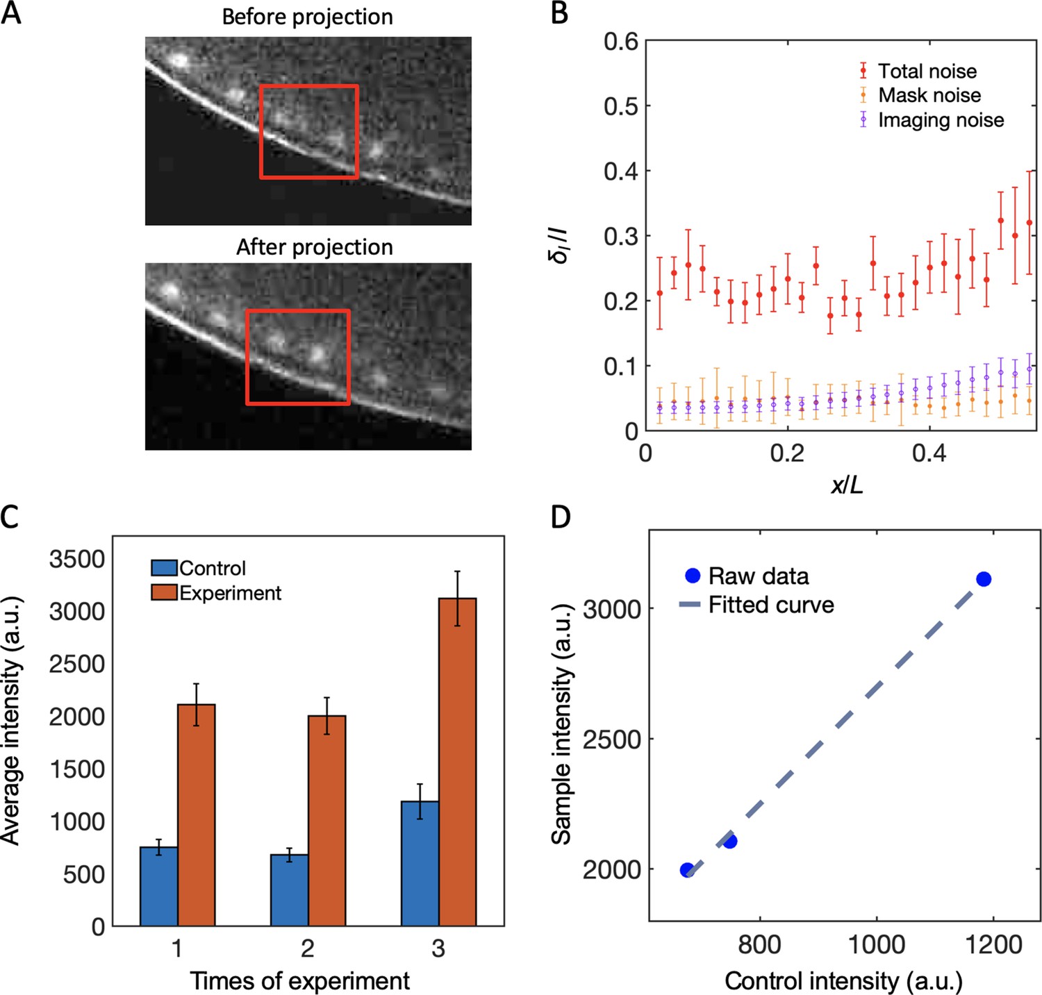
Live imaging of dynamic Bcd gradients.
(A) Comparison of the maximum projected image and the single image in the mid-sagittal plane from a z-stack of images of the fly embryos expressing Bcd-GFP in nc12. (B) The nuclear mask noise from imaging segmentation and the imaging shot noise is much smaller than the total Bcd-GFP gradient noise. (C) Comparison of the average nuclear fluorescence intensity of the control sample and the embryos measured in three independent sessions. (D) The average nuclear fluorescence intensity of the embryos is linearly correlated with that of the control sample in three measurement sessions. Blue circles represent data from each session, and the dash line represents the linear fitting.
Figure 3 with 1 supplement
The activation of Hb by Bcd is consistent with the threshold-dependent model in stau– mutants at early nc14.
Comparison of the Bcd concentration (horizontal lines) at xHb (vertical lines) at 16 min into nc14 between stau– mutants (blue) and the WT (black) before (inset) and after maturation correction on the Bcd gradient. Each circle and error bar represent the average and standard deviation, respectively, of the Bcd-GFP fluorescence intensity of the nuclei in the bin with a bin size of 2% EL.
-
Figure 3—source data 1
Source data for Figure 3.
- https://cdn.elifesciences.org/articles/54276/elife-54276-fig3-data1-v2.xlsx
Figure 3—figure supplement 1
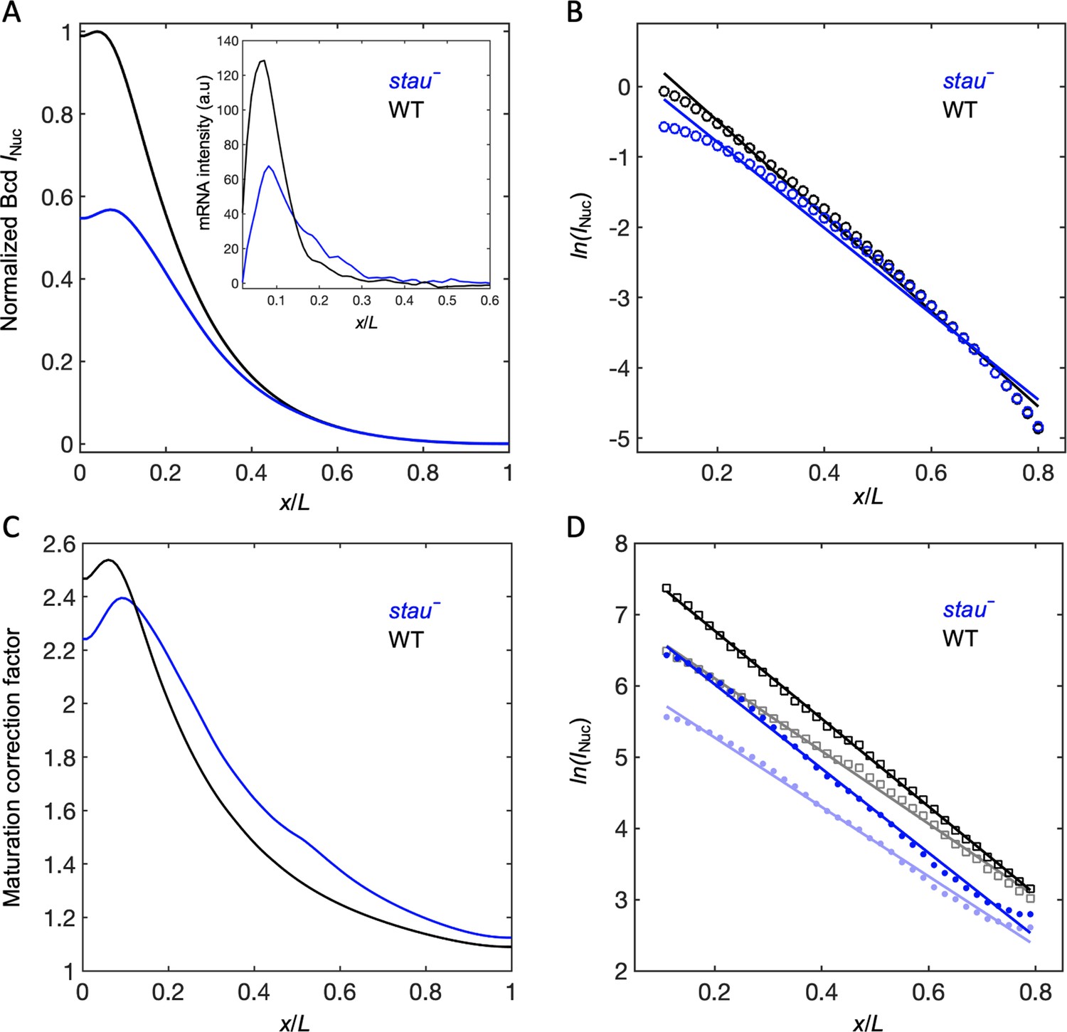
Maturation correction on Bcd-GFP gradients.
(A) The simulated steady-state Bcd gradient of the WT (black) and stau– mutants (blue) based on the model with the extensive distributed source of mRNA extracted from the reference (Petkova et al., 2014). (B) The logarithm of the intensity of the simulated Bcd gradient in panel (A) as a function of the fractional embryo length. The linear fits show that the apparent length constants are 15% of EL and 17% of EL for the WT and stau– mutants, respectively. (C) Maturation correction curves of the Bcd gradient. (D) The logarithm of the intensity as a function of the fractional embryo length and the linear fit before maturation correction (light color) and after maturation correction (dark color).
Figure 4 with 3 supplements
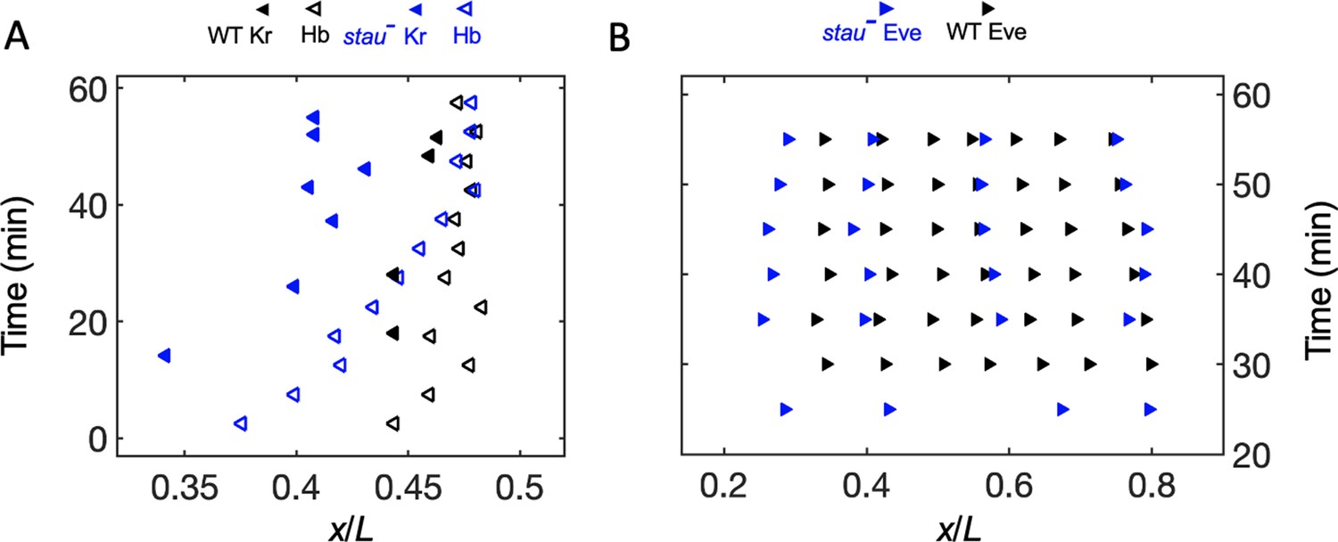
The dynamic shift range of the position of Kr and Eve is smaller than that of Hb in stau– mutants.
(A) The positions of the anterior boundary (inflection point) of Kr (solid triangle) and xHb (hollow triangle) with the stau– mutants (blue) and the WT (black). (B) The peak of Eve in stau– mutants (blue) as a function of the developmental time in nc14 in comparison with that in the WT (black).
-
Figure 4—source data 1
Source data for Figure 4.
- https://cdn.elifesciences.org/articles/54276/elife-54276-fig4-data1-v2.xlsx
Figure 4—figure supplement 1
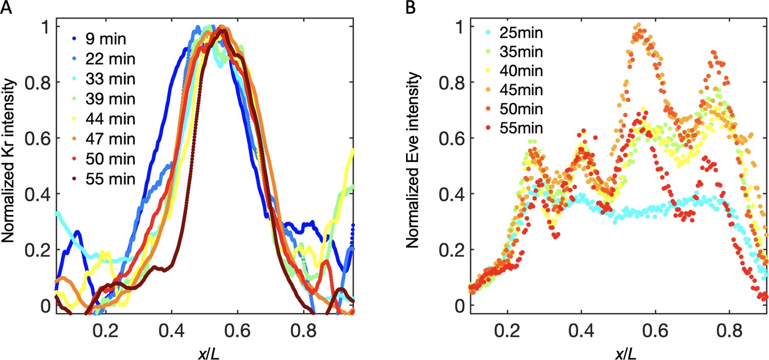
Measurement results of Kr and Eve in stau– mutants.
(A, B) Dynamics of the Kr (A) and Eve (B) profiles in nc14.
Figure 4—figure supplement 2
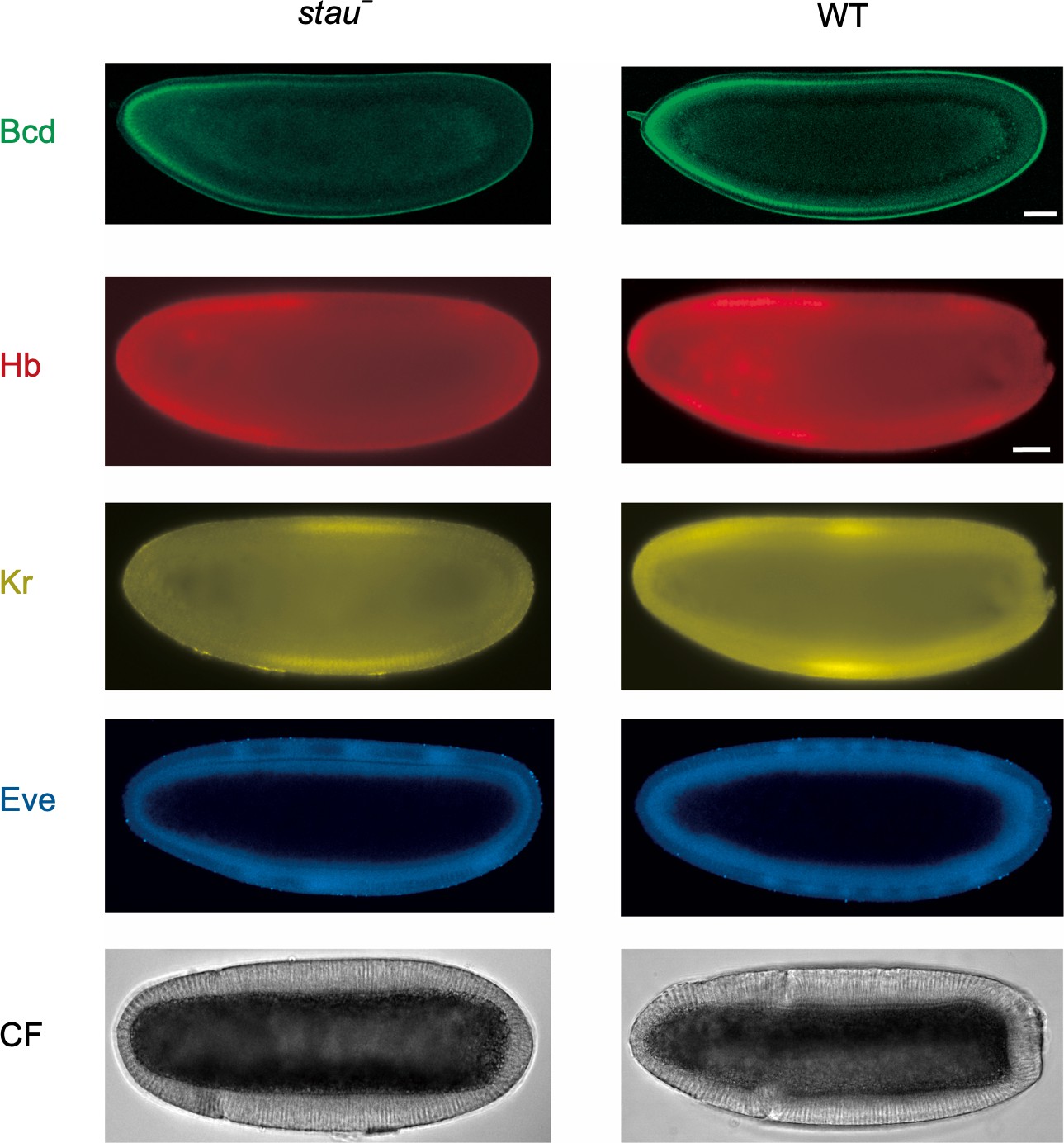
Representative raw images of Bcd-GFP, Hb, Kr, Eve, and CF of the WT and stau– mutants.
Representative raw images of Bcd-GFP (green), Hb (red), Kr (yellow), Eve (blue), and CF (black) of stau– mutants (left) and the WT (right). The top two figures are living images of Bcd-GFP at 16 min into nc 14, and the next three rows of figures are the immunofluorescence images of Hb, Kr, and Eve at around 35 min into nc 14. The last row is the bright field image of CF at around 56 min into nc 14. The scale bars represent 40 μm. The first scale bar is for the top two images and the second one for the rest. The second scale bar is slightly longer due to shrinkage after heat fixation.
Figure 4—figure supplement 3
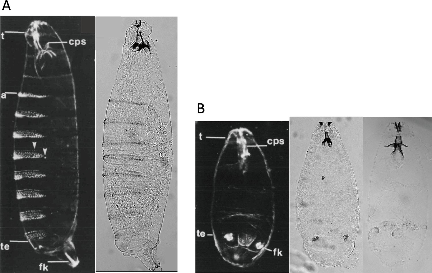
Cuticle patterns of stau– mutants.
Cuticle patterns of the stau– mutants prepared with CRISPR are consistent with the published record (Lehmann and Nüsslein-Volhard, 1991). (A) Comparison of the dark field image of the cuticle pattern of the WT in Lehmann and Nüsslein-Volhard, 1991 and the bright field image of the WT in our experiment. (B) Comparison of the dark field image of the cuticle pattern of stau– mutants in Lehmann and Nüsslein-Volhard, 1991 and the bright field images of stauD3 and stauHL54 prepared with CRISPR technique.
Figure 5 with 1 supplement
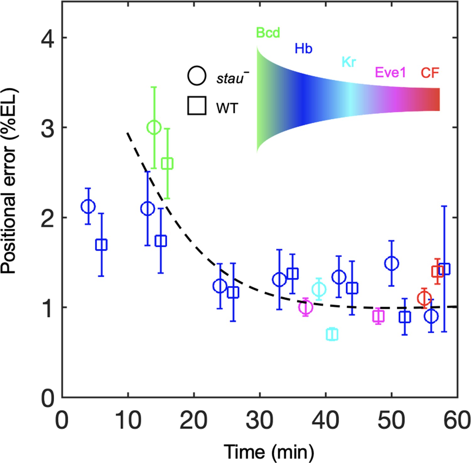
Positional noise is filtered from Bcd to CF.
Positional errors in Bcd (green), Hb (blue), Kr (cyan), Eve (magenta) and CF (red) of stau– mutants (circle) and the WT (square) as a function of developmental time in nc14. Positional errors are calculated from the Bcd gradients (Figure 2A) after subtracting the imaging noise and image mask noise from the gradient noise (Figure 2B). The standard deviation of the average positional noise is calculated on the basis of bootstrapping. For presentation purposes, data for Bcd, Kr and CF measured at the same time point are shown with 1 min offset on the x axis. The black line connects the data points to guide the eye.
-
Figure 5—source data 1
Comparison of the minimal positional errors of patterning markers.
Source data for Figure 5.
- https://cdn.elifesciences.org/articles/54276/elife-54276-fig5-data1-v2.docx
Figure 5—figure supplement 1
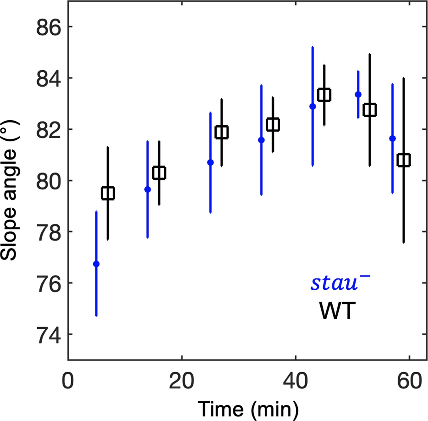
Dynamics of the average Hb boundary slopes.
The average Hb boundary slopes of the stau– mutants (blue circle) and the WT (black circle) as a function of the developmental time in nc14, error bars denote the standard deviation of each bin with the same sample size (n=10 and 7 except the last bin for stau- mutants and the WT, respectively). The time points of the WT have a 1 min offset along the time axis for visual display.
Figure 6 with 1 supplement
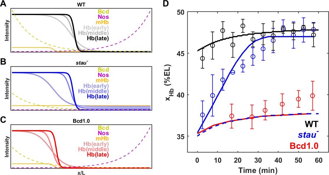
Origin of the large shift in xHb in stau– mutants.
(A–C) Schematic of maternal gradients and Hb dynamic expression in the WT (A), stau– mutants (B), and Bcd1.0 (C). In stau– mutants, the Bcd gradient (yellow) decreases in amplitude and increases in length constant. The depletion of the Nos gradient (purple) flattens the maternal Hb gradient (orange). In Bcd1.0, the Bcd gradient decreases in amplitude by half. xHb moves posteriorly from early, to middle and late nc14. It mainly moves in the first 30 mins in nc14 in stau– mutants and the shift amount is much greater than in the WT. By contrast, xHb mainly moves in the later 30 mins of nc14 in Bcd1.0. (D) The mathematical model fitting (lines) agrees well with the measured shift of xHb in the WT (black circles) and stau– mutants (blue circles), but not Bcd1.0 (red circles). The simulation result without the distortion effect on the Nos gradient in stau– mutants (blue dashed line) fails to replicate the measured results. Error bars represent the standard deviation of xHb in each time window.
-
Figure 6—source data 1
Model parameters.
- https://cdn.elifesciences.org/articles/54276/elife-54276-fig6-data1-v2.docx
-
Figure 6—source data 2
Source data for Figure 6 and Figure 6—figure supplement 1.
- https://cdn.elifesciences.org/articles/54276/elife-54276-fig6-data2-v2.xlsx
Figure 6—figure supplement 1
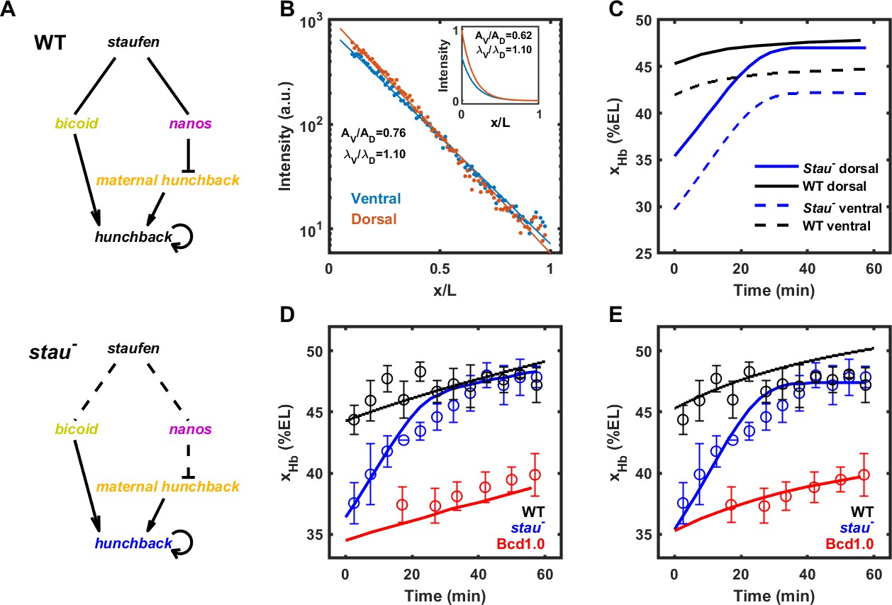
Mathematical modeling of the shift of xHb.
(A) The regulation network of maternal genes and Hb in the WT (top) and in stau– mutants (below). The arrow (→) and the T-bar (—|) symbols represent activation and repression, respectively. The dashed line represents the missing regulatory interactions. (B) Comparison of the measured average Bcd gradient (n = 11) on the ventral side (blue dots) and the dorsal (red dots) side. The fitting results (lines) show that the amplitude decreases from 1078 on the dorsal side by 24% to 814 on the ventral side, whereas the length constant increases from 19.0% EL on the dorsal side by 10% to 21.0% EL on the ventral side. Inset: the dorsal and ventral Bcd gradients in the simulation with the best-fitting result. (C) The simulated xHb on the ventral side (dashed line) posteriorly moves 6% EL and 3% EL compared with the dorsal side (solid line) in stau– mutants (blue) and the WT (black). (D, E) After removing the time-varying effect of Bcd gradients, the mathematical model fitting (lines) of xHb does not stabilize in the late nc14 in the WT (black circles) or in stau– mutants (blue circles) as shown in the experiment whether using the updated (D) or same (E) optimized parameters. Error bars represent the standard deviation of xHb in each time window.
Author response image 1
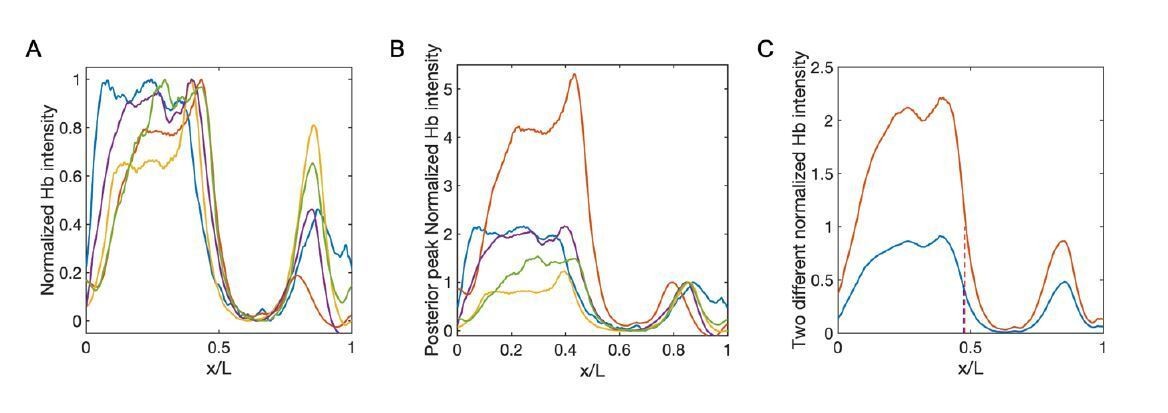
Comparison between conventional normalized method and the normalization using the posterior peak as the reference.
(A–B) Normalized profiles of Hb intensity of stau– mutants in one developmental time window (45-50 min into nc14, sample number: n = 5) using the conventional method (A) and posterior peak normalization method (B). Different colors represent different samples. (C) The average profile of Hb intensity with the conventional method (A, blue) and posterior-peak-normalization method (B, red). The boundary positions are 47.4% EL (blue) and 47.8% EL (red), respectively.
Tables
Key resources table
| Reagent type (species) or resource | Designation | Source or reference | Identifiers | Additional information |
|---|---|---|---|---|
| Strain, strain background (D. melanogaster) | w1118 | Yi Rao Lab | BDSC3605 | |
| Strain, strain background (D. melanogaster) | stauHL54 | This paper | See 'Materials and methods' | |
| Strain, strain background (D. melanogaster) | stauD3 | This paper | See 'Materials and methods' | |
| Strain, strain background (D. melanogaster) | bcd-egfp;+;bcdE1 | Thoms Gregor Lab | ||
| Strain, strain background (D. melanogaster) | bcd-egfp;stauHL54;bcdE1 | Thoms Gregor Lab | ||
| Antibody | Anti-Hb (mouse monoclonal) | Abcam | ab197787 | IF (1:1000) |
| Antibody | Anti-Kr (guinea pig polyclonal) | John Reinitz Lab | IF (1:1000) | |
| Antibody | Anti-Eve (rat polyclonal) | John Reinitz Lab | IF (1:1000) | |
| Antibody | Anti-guinea pig (goat monoclonal) | John Reinitz Lab | IF (1:1000) | |
| Antibody | Anti-rat (goat monoclonal) | Invitrogen | A11006 | IF (1:1000) |
| Antibody | Anti-mouse (goat monoclonal) | Invitrogen | A21240 | IF (1:1000) |
| Chemical compound, drug | Agarose gels | Invitrogen | E-Gel EX | 1~1.5% |
| Software, algorithm | 3D image processing | This paper | Source code files | See 'Materials and methods' |
| Software, algorithm | MATLAB | MATLAB, 2018 | MATLAB 2018a v9.4.0.813654 | |
| Other | DAPI stain | Invitrogen | D1306 | (1 µg/mL) |
| Other | Capillary | Brand | 701904 |
Additional files
-
Source code 1
3D imaging analysis code.
- https://cdn.elifesciences.org/articles/54276/elife-54276-code1-v2.zip
-
Transparent reporting form
- https://cdn.elifesciences.org/articles/54276/elife-54276-transrepform-v2.docx
Download links
A two-part list of links to download the article, or parts of the article, in various formats.
Downloads (link to download the article as PDF)
Open citations (links to open the citations from this article in various online reference manager services)
Cite this article (links to download the citations from this article in formats compatible with various reference manager tools)
The dynamic transmission of positional information in stau- mutants during Drosophila embryogenesis
eLife 9:e54276.
https://doi.org/10.7554/eLife.54276


