Figures and data in Coverage-dependent bias creates the appearance of binary splicing in single cells

Figures
Tables
Additional files

4 figures, 2 tables and 1 additional file

Figures

Figure 1

Download asset Open asset

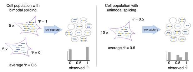
Bimodal vs unimodal models of cassette exon splicing.

In the bimodal model, some cells consistently splice in the exon, while others consistently skip it. After mRNA capture and sequencing, observations of $Ψ$ are almost exclusively binary. In the unimodal model, individual cells express some mRNAs that splice in the cassette exon and some that skip it. Low mRNA capture dramatically reduces the number of cells in which both isoforms are observed, artificially inflating binary $Ψ$ values.

Figure 2 with 1 supplement

Download asset Open asset

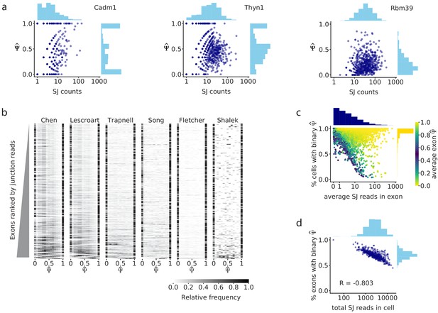
Splice junction read coverage is correlated with unimodality of splicing distributions.

(a) Comparison of splice junction read coverage and observed $\hat{Ψ}$ for three cassette exons in the Chen dataset, with low (Cadm1 exon 8; chr9: 47829377–47829409), medium (Thyn1 exon 6, chr9: 27006801–27006951), and high coverage (Rbm39 exon 3; chr2: 156178880–156178952). Each dot represents the $\hat{Ψ}$ of that exon in one cell. (b) $\hat{Ψ}$ distribution of the 300 highest coverage cassette exons with intermediate splicing (average $\hat{Ψ}$ between 0.2 and 0.8) in each of the six analyzed datasets. Each row in the heatmap shows the distribution of $\hat{Ψ}$ for one exon across all cells. (c) Relationship between the average read coverage and proportion of binary observations for each cassette exon in the Chen dataset. (d) Correlation between the total number of splice junction reads captured in each cell, and proportion of cassette exons with intermediate splicing that show binary $\hat{Ψ}$ in that cell.

Figure 2—figure supplement 1

Download asset Open asset

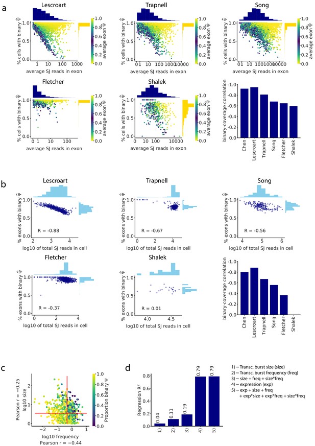
Junction read coverage determines the proportion of binary observations in all analyzed datasets.

(a) As in Figure 2c, the splice junction read coverage of an intermediate exon was anti-correlated with the proportion of cells in which it shows binary $\hat{Ψ}$ (only one isoform is observed) in all datasets. Barplot: Pearson correlation between read coverage and proportion of binary observations of each cassette exon. (b) As in Figure 2d, the total number of splice junction reads in a cell was inversely proportional to the fraction of exons that have binary values in the cell in all datasets. Barplot: Pearson correlation between the total number of captured reads in each cell and the proportion of cassette exons with binary $\hat{Ψ}$ . (c) Relationship between transcriptional burst frequency and size, and the proportion of binary observations of an exon. (d) $R^{2}$ of the linear regression prediction of the proportion of binary observations per exon based on burst frequency, size, number of reads, and a combination of these features.

Figure 3 with 2 supplements

Download asset Open asset

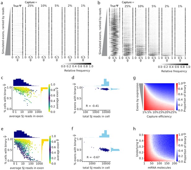
Simulations show that gene expression and capture efficiency influence the observed distribution of splicing.

(a) Simulations of alternative splicing and scRNA-seq under the binary-bimodal model, in which each cell produces one isoform or the other, but rarely both. As in Figure 2b, each row of the histogram shows $\hat{Ψ}$ for one intermediate exon across all cells. The observed $\hat{Ψ}$ distribution is similar to the true $Ψ$ distribution, and its shape is largely unaffected by capture efficiency. (b) Simulations with the non-binary, unimodal model, in which most cells present a mixture of the two alternative isoforms. Exons with high expression have a unimodal distribution of true $Ψ$ . Low capture efficiency results in an increase in binary observations (only one isoform observed), leading to a distortion of the observed distribution of $\hat{Ψ}$ to look bimodal. Only a handful of the highest expressed exons maintain a unimodal distribution of $\hat{Ψ}$ . Fewer exons show unimodal splicing as the capture efficiency is reduced. (c) Under the binary-bimodal model, exons with high coverage have slightly fewer binary $Ψ$ observations, and (d) simulated cells with a high number of total splice junction reads have slightly fewer exons with binary $\hat{Ψ}$ . (e) Under the unimodal model, exons with intermediate splicing show a strong decrease in binary observations as coverage increases, as seen in real data (Figure 2c). (f) Similarly, simulated cells with high read coverage have a decrease of the proportion of binary $\hat{Ψ}$ . (g) Effect of capture efficiency on the proportion of binary observations of cassette exons with underlying $Ψ$ = 0.5. (h) Effect of the initial number of mRNA molecules and underlying $Ψ$ on the proportion of binary $\hat{Ψ}$ observations.

Figure 3—figure supplement 1

Download asset Open asset

Theoretical calculations and simulations of the effect of biological and technical factors in splicing observations.

(a) Theoretical likelihood of capturing only mRNAs representing one isoform of an alternatively spliced gene in a single cell, determined by the total number of mRNAs in the cell, the $Ψ$ of the isoforms, and a 10% capture efficiency. (b) Probability of observing a binary $\hat{Ψ}$ (only one isoform observed) given the number of mRNA molecules of that gene present in the cell, when the underlying $Ψ$ is fixed at 0.5. (c) Effect of the number of captured mRNA molecules on the uncertainty of $\hat{Ψ}$ observations. $\hat{Ψ}$ is understood as the maximum likelihood estimate of the underlying $Ψ$ . (d) The posterior probability of having an observed $\hat{Ψ}$ within 0.1 of the underlying $Ψ$ . (e) Distribution of the relative error between the average observed $\hat{Ψ}$ , and the average true $Ψ$ , in our simulations under different capture efficiency rates. The relative error is calculated as the difference between the average $\hat{Ψ}$ and the average true $Ψ$ , scaled by the average true $Ψ$ . (f) Distribution of the relative error between the variance in the observed $\hat{Ψ}$ , and the variance in the true $Ψ$ , in our simulations under different capture efficiency rates.

Figure 3—figure supplement 2

Download asset Open asset

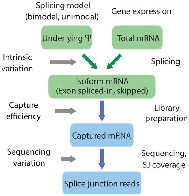
Schematic of scRNA-seq splicing simulator.

Simulator of scRNA-seq splicing data. Green elements represent biological variables; blue elements represent technical processes. The underlying $Ψ$ is drawn from a Beta distribution with either a bimodal or unimodal shape. Individual gene expression determines the total number of mRNAs, and these mRNAs are spliced stochastically according to $Ψ$ , producing isoforms that splice in or skip the exon. mRNAs are captured with a probability drawn from a normal distribution. Sequencing produces splice junction reads, which determine the observed $\hat{Ψ}$ .

Figure 4 with 4 supplements

Download asset Open asset

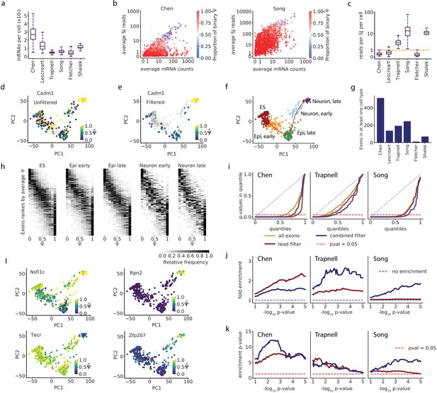
Accounting for coverage biases reveals unimodal splicing distributions and differential splicing.

(a) Estimated total mRNA molecules captured per cell. (b) Estimated number of recovered mRNAs vs splice junction reads for cassette exons, averaged across cells. Each dot corresponds to an exon, and its color indicates the proportion of cells in which it has a binary observation (only one isoform observed). We analyzed exons with average $\hat{Ψ}$ between 0.05 and 0.95. (c) Per-cell splice junction coverage rate in each dataset. (d) Cadm1 exon 8 alternative splicing appears binary in many cells in the Chen dataset. Correlation with lineage pseudotime: Spearman’s $r_{s}$ = 0.1. (e) Cadm1 exon after removing cells with fewer than 10 recovered Cadm1 mRNA molecules and fewer splice junction reads than expected from 10 mRNAs (grey). Spearman’s $r_{s}$ = 0.52. (f) PCA projection and clustering of single cells in the Chen dataset, showing differentiation of mouse ES cells into neurons. Red line, lineage inferred with Slingshot. (g) Number of cassette exons with observations from at least 10 mRNA reads in at least 50% of cells in any cluster. (h) Stacked histograms showing the distribution of observed $\hat{Ψ}$ of exons as in (g), in each cell cluster of the Chen dataset. Observations with fewer than 10 mRNA molecules were removed. We show exons with average $\hat{Ψ}$ ranging from 0.1 to 0.9 per cluster. (i) QQ-plot comparing the quantiles of a uniform distribution (x-axis) with the quantiles of the distributions of p-values from the Kruskal-Wallis test (y-axis). A diagonal line (gray dotted line) would mean the p-values are uniformly distributed. A lower area under the curve indicates enrichment for low p-values. The point on the x-axis at which each line crosses the dotted red line indicates the proportion of p-values that are below 0.05 in the distribution. (j) Fold enrichment of exons with a Kruskal-Wallis p < $x$ in the set of exons selected with the mRNA-based filter (blue), and exons selected with a flat read minimum filter (red). (k) Significance p-value of the enrichment, estimated with the hypergeometric test and adjusted for FDR. (l) Example exons that pass the overall filter criteria in the Chen dataset and have p<0.05 in the Kruskal-Wallis test.

Figure 4—figure supplement 1

Download asset Open asset

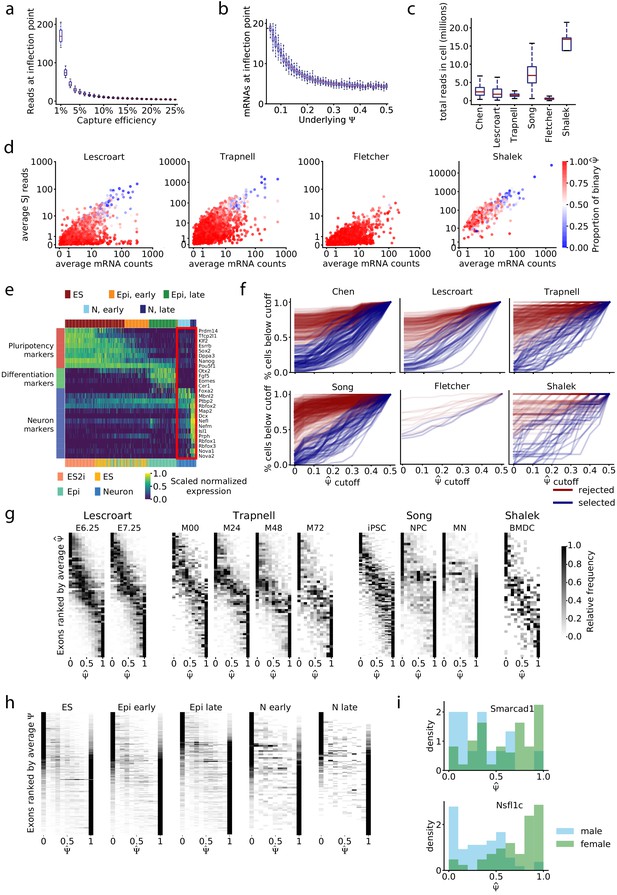
Relationship between read coverage, captured mRNAs, and binarity in single cell datasets.

(a) Average number of splice junction reads required to have a 50% likelihood of observing both isoforms, from simulations in Figure 3j. (b) Total mRNAs required to have a 50% likelihood of observing both isoforms, from simulations in Figure 3k. (c) Total mapped reads per cell for each dataset. (d) Estimated average number of recovered mRNAs vs. average number of splice junction reads for each exon. (e) Expression of pluripotency and neuron differentiation marker genes in the Chen dataset; expression is scaled by each row’s maximum and minimum. Cells are ordered by inferred pseudotime. Top color key, clusters from agglomerative clustering; bottom color key, labels from Chen et al. The red box highlights two sub-groups of neurons identified by clustering. (f) Visualization of the distribution of $\hat{Ψ}$ observations toward extreme values in the first cluster of cells of each dataset. For each $x$ cutoff in the x-axis, the y-axis corresponds to the proportion of cells that have $\hat{Ψ} \leq x$ or $\hat{Ψ} \geq (1 - x)$ . Blue lines, exons passing the mRNA-based filter; red lines, exons removed by filter. (g) Stacked histograms, as in Figure 4h, for other datasets. The Fletcher dataset is excluded because only five exons pass the mRNA filter. (h) Stacked histograms of exons that do not pass the filter in the Chen dataset; exons were subsampled to match the number that do pass the filter in each cell type cluster. (i) Sex-dependent distribution of $\hat{Ψ}$ of the two bimodal exons of the Chen dataset after cell-type stratification: Smarcad1 exon 3 (chr6: 65043836–65044108) in early Epi cells, Nsfl1c exon 4 (chr2: 151502455–151502460) in late Epi cells.

Figure 4—figure supplement 2

Download asset Open asset

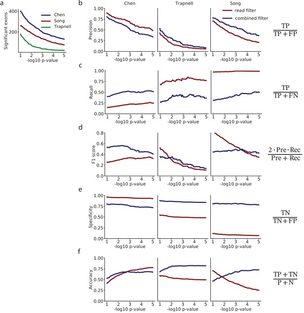
Analysis of differential splicing among selected exons with the Kruskal-Wallis analysis of variance.

(a) Comparison of the precision of selecting exons with low p-values, for the mRNA-based filter versus selecting exons on a flat minimum of 10 reads. (b) Recall. (c) F1-score. (d) Specificity. (e) Accuracy. (f) Number of exons with $p \leq x$ in each dataset.

Figure 4—figure supplement 3

Download asset Open asset

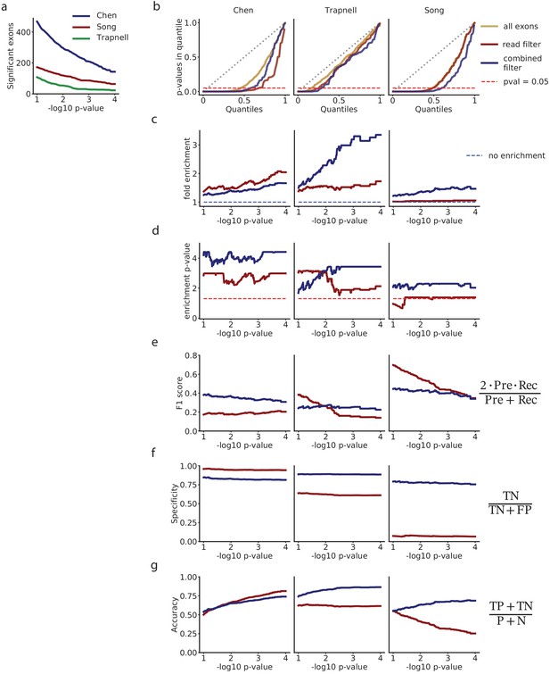
Analysis of differential splicing among selected exons with the autocorrelation test.

(a) Number of exons with p $\leq x$ in each dataset. (b) QQ-plot comparing the quantiles of a uniform distribution, with the quantiles of the distributions of p-values from the autocorrelation test. (c) Fold enrichment of exons with an autocorrelation p < $x$ in the set of exons selected with the mRNA-based filter (blue), and exons selected with a flat read minimum filter (red). (d) Significance p-value of the enrichment shown in (c). For each p-value limit $x$ , we estimate the significance with the hypergeometric test, and correct for multiple testing using the Benjamini-Hochberg FDR adjustment. (e) F1-score. (f) Specificity. (g) Accuracy.

Figure 4—figure supplement 4

Download asset Open asset

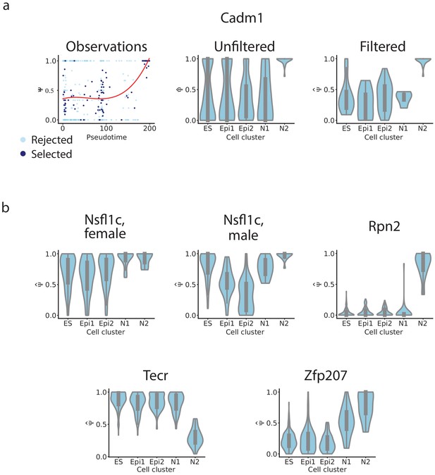
Distribution of $\hat{Ψ}$ of example exons.

(a) Skipped Cadm1 exon 8 (chr9: 47829377–47829409). We show the relationship between pseudotime and observed $\hat{Ψ}$ ; as well as violinplots of the distribution of $\hat{Ψ}$ in each cluster before filtering, and after filtering. (b) Violinplots of the distribution of $\hat{Ψ}$ in each cluster after filtering for the exons in Figure 4k: Nsfl1c exon 4 (chr2: 151502455–151502460), Rpn2 exon 16 (chr2: 157323223–157323270), Tecr exon 4 (chr8: 83573411–83573455), Zfp207 exon 8 (chr11: 80393084–80393176).

Tables

Table 1

Prevalence of bimodal splicing distributions before and after filtering.

Dataset	Cell type cluster	Cells	Exons	Bimodal	% bimodal	Selected	Selected bimodal	% bimodal selected	p-val (adj)
Chen	ES	217	446	118	26%	94	0	0%	3.3e-14
Chen	Epi, early	98	402	107	27%	98	1	1%	9.3e-14
Chen	Epi, late	104	516	136	26%	76	1	1%	1.1e-09
Chen	Neuron, early	47	364	117	32%	43	0	0%	3.6e-08
Chen	Neuron, late	22	517	146	28%	61	0	0%	1.1e-09
Lescroart	Heart E6.75	172	286	77	27%	33	0	0%	2.0e-05
Lescroart	Heart E7.25	341	291	78	27%	36	0	0%	8.0e-06
Trapnell	Myoblast 00 hr	35	400	142	36%	41	0	0%	1.2e-08
Trapnell	Myoblast 24 hr	89	251	97	39%	27	0	0%	1.2e-06
Trapnell	Myoblast 48 hr	72	242	97	40%	32	1	3%	9.1e-07
Trapnell	Myoblast 72 hr	35	252	101	40%	24	1	4%	5.1e-05
Song	iPSC	62	616	269	44%	55	0	0%	3.3e-14
Song	NPC	73	212	92	43%	28	1	4%	1.2e-06
Song	MN	67	168	82	49%	19	4	21%	9.4e-03
Shalek	BMDC	13	149	51	34%	27	1	4%	6.6e-05

Table 2

Single-cell RNA-seq datasets.

Dataset	Organism	Biological process	Cells	No. ASE	Mean reads/event	Protocol	Accession	Reference
Chen	mouse	mES neuron differentiation	488	3276	3.1	Smart-seq2	GSE74155	Chen et al., 2016
Lescroart	mouse	cardiomyogenesis	598	3007	3.2	Smart-seq2	GSE100471	Lescroart et al., 2018
Trapnell	human	skeletal myogenesis	314	4457	14.4	Smart-seq	GSE52529	Trapnell et al., 2014
Song	human	iPS motor neuron differentiation	206	5355	88.8	Smart-seq	GSE85908	Song et al., 2017
Fletcher	mouse	olfactory neurogenesis	849	684	2.7	Smart-seq	GSE95601	Fletcher et al., 2017
Shalek	mouse	bone-marrow-derived dendritic cells	18	380	213.4	Smart-seq	GSE41265	Shalek et al., 2013

Additional files

Transparent reporting form: https://cdn.elifesciences.org/articles/54603/elife-54603-transrepform-v2.pdf
Download elife-54603-transrepform-v2.pdf

Download links

A two-part list of links to download the article, or parts of the article, in various formats.

Downloads (link to download the article as PDF)

Open citations (links to open the citations from this article in various online reference manager services)

Mendeley

Cite this article (links to download the citations from this article in formats compatible with various reference manager tools)

Carlos F Buen Abad Najar
Nir Yosef
Liana F Lareau

(2020)

Coverage-dependent bias creates the appearance of binary splicing in single cells

eLife 9:e54603.

https://doi.org/10.7554/eLife.54603

Share this article

Cite this article

Bimodal vs unimodal models of cassette exon splicing.

Splice junction read coverage is correlated with unimodality of splicing distributions.

Junction read coverage determines the proportion of binary observations in all analyzed datasets.

Simulations show that gene expression and capture efficiency influence the observed distribution of splicing.

Theoretical calculations and simulations of the effect of biological and technical factors in splicing observations.

Schematic of scRNA-seq splicing simulator.

Accounting for coverage biases reveals unimodal splicing distributions and differential splicing.

Relationship between read coverage, captured mRNAs, and binarity in single cell datasets.

Analysis of differential splicing among selected exons with the Kruskal-Wallis analysis of variance.

Analysis of differential splicing among selected exons with the autocorrelation test.

Distribution of Ψ^ of example exons.

Prevalence of bimodal splicing distributions before and after filtering.

Single-cell RNA-seq datasets.

Transparent reporting form

Downloads (link to download the article as PDF)

Open citations (links to open the citations from this article in various online reference manager services)

Cite this article (links to download the citations from this article in formats compatible with various reference manager tools)

Distribution of $\hat{Ψ}$ of example exons.